Predictive Modeling of a Leaf Conceptual Midpoint Quasi-Color (CMQ) Using an Artificial Neural Network
←
→
Page content transcription
If your browser does not render page correctly, please read the page content below
sensors
Article
Predictive Modeling of a Leaf Conceptual Midpoint
Quasi-Color (CMQ) Using an Artificial
Neural Network
Ivan Simko
 U.S. Department of Agriculture, Agricultural Research Service, U.S. Agricultural Research Station,
 Crop Improvement and Protection Research Unit, Salinas, CA 93906, USA; ivan.simko@usda.gov

 Received: 9 June 2020; Accepted: 14 July 2020; Published: 15 July 2020

 Abstract: The color of plant leaves is moderated by the content of pigments, which can show
 considerable dorsiventral distribution. Two typical examples are leafy vegetables and ornamentals,
 wherein red and green color surfaces can be seen on the same leaf. The proof of concept is provided for
 predictive modeling of a leaf conceptual mid-point quasi-color (CMQ) from the content of pigments.
 The CMQ idea is based on the hypothesis that the content of pigments in leaves is associated with the
 combined color from both surfaces. The CMQ, which is calculated from CIELab color coordinates at
 adaxial and abaxial antipodes, is thus not an actual color, but a notion that can be used in modeling.
 The CMQ coordinates, predicted from the content of chlorophylls and anthocyanins by means of
 an artificial neural network (ANN), matched well with the CMQ coordinates empirically found on
 photosynthetically active leaves of lettuce (Lactuca sativa L.), but also with other plant species with
 comparable leaf attributes. Modeled values of lightness (qL*) decreased with the increasing content
 of both pigments, while the redness or greenness (qa*) and yellowness or blueness (qb*) of the CMQ
 were affected more by a relative content of chlorophylls and anthocyanins in leaves. The highest
 vividness of quasi-colors (qC*) was modeled for leaves with a high content of either pigment alone.
 The model predicted a substantially duller quasi-color for leaves with chlorophylls and anthocyanins
 present together, particularly when both pigments were present at very high levels.

 Keywords: anthocyanins; artificial neural network; chlorophylls; leaf color; plant pigments; predictive
 modeling

1. Introduction
     The pigments in plant leaves play a critical role in biological functions, such as capturing light
energy for photosynthesis or mitigating stresses caused by biotic and abiotic factors [1]. The amount
and combination of pigments in leaves affects visual perception of their color, the trait that is vital to
consumers of leafy vegetables and growers of ornamental plants. Moreover, plant pigments have a
beneficial effect on human health [1], making them a highly desirable target of plant breeding programs.
Plant phenotyping is a rapidly growing research area that utilizes sensors to nondestructively monitor
plant traits [2,3], including evaluations of leaf color and leaf pigment content that can provide helpful
insight into the physiological performance of leaves [4]. The three basic types of pigments that
cause leaf coloration are chlorophylls (green color), anthocyanins (red–purple color) and carotenoids
(yellow–orange color), though the bright color of carotenoids is usually masked in photosynthetically
active tissues and revealed only after the degradation of chlorophylls occurs [5]. Combinations of
these plant pigments were used for modeling virtual [6–10] or real colors of fruits, vegetables [11],
leaves [12], and the mechanism of color change [13]. For example, the color of leaves and its change
were modeled using simulated concentrations of chlorophylls, carotenes and anthocyanins [10],

Sensors 2020, 20, 3938; doi:10.3390/s20143938                                     www.mdpi.com/journal/sensors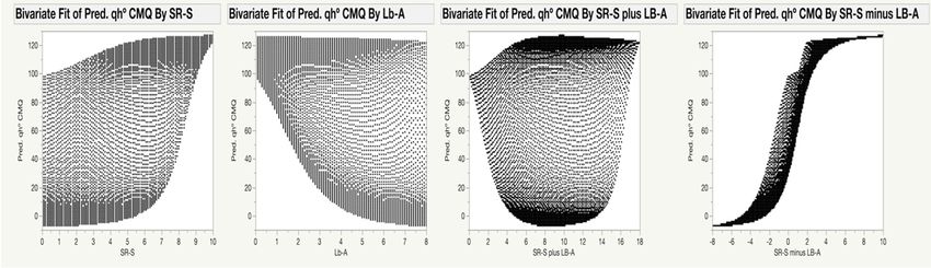
Sensors 2020, 20, 3938                                                                                 2 of 15

or actual concentrations of chlorophylls and carotenes [7]. In simple systems, where only one pigment
is predominant, a strong relationship between concentrations of this pigment and color may be
observed [11], e.g., between chlorophylls and a green color [9,14] or between anthocyanins and red a
color [15,16]. However, in more complex systems, wherein multiple pigments occur within the same
tissue, these simple relationships cease to be visible [11] due to spectral inference between pigments [4].
      Leaf color can be defined using the CIELab color space that approximates human visual
perception [17]. This color space is characterized by three coordinates: L*, a* and b*. L* indicates
lightness of color and ranges from 0 (minimum, darkest black) to 100 (maximum, brightest white),
a* indicates redness (positive values) or greenness (negative values), while b* indicates yellowness
(positive values) or blueness (negative values) √ of color. The combination of a* and b*∗ coordinates
provides information about chroma (C* = a∗2 + b∗2 ) and hue angle (h◦ = arctan ( ba∗ )). Chroma
describes vividness of the color, with higher values indicating more vivid (less dull) color, while
the hue angle is associated with the dominant color as perceived by an observer. The hue angle
values are usually defined as red–purple at 0◦ , yellow at 90◦ , bluish-green at 180◦ , and blue at 270◦ .
The difference
           √ between two colors (∆E) can be calculated from changes at each of the three coordinates
as: ∆E = ∆L2 + ∆a2 + ∆b2 .
      CIELab or other color space (e.g., RGB) coordinates were previously corelated with the content of
either chlorophylls [9,14] or anthocyanins [15,16], but were not investigated on leaves with varying
contents of both pigments combined. Moreover, these analyses were performed using statistical
models with restrictive structural assumptions. It is also important to note that most of the published
associations between leaf color and color coordinates were performed on only a single leaf surface
(usually adaxial) [14,15], though a large number of plant species have bifacial leaves that show
substantial dorsiventral distribution of pigments. Lettuce, the most popular commercially produced
leafy vegetable [18], is a typical example of diversity in leaf color across cultivars, but also between two
leaf surfaces. The color can range from very light green to dark green, and from very light red to dark
red, to almost black [19]. These large variations make the modeling of lettuce leaf color challenging
because the content of pigments cannot be unambiguously associated with the color on either one of
the surfaces.
      To assess the association between pigments and the color on leaves showing dorsiventral
distribution, the color on both leaf surfaces needs to be considered. It could be hypothesized that the
amount of pigments in leaves, particularly in cases where differences in pigment and color distribution
between adaxial and abaxial surfaces are substantial, would match more accurately with combined
color coordinates from both surfaces, rather than with color coordinates from only one of the surfaces.
The combining of color coordinates can be done through the concept of ‘quasi-color’ at ‘mid-point’.
Mid-point is a conceptual point between two antipodal points on leaf adaxial and abaxial surfaces,
which combines color coordinates from both of them. The conceptual mid-point quasi-color (CMQ)
is thus not an actual color of the leaf, but a notion that can be used in modeling. The qL*, qa* and
qb* vector coordinates of the CMQ are calculated from two three-dimensional vector coordinates of
                         L∗ + L∗   a∗ + a∗       b∗ +b∗
color at antipodes, as: ( D 2 B ), ( D 2 B ) and ( D 2 B ), where L*, a* and b* are the color coordinates for
antipodal points that are located on adaxial (subscript D) and abaxial (subscript B) surfaces. Quasi-color
chromaticity (qC*) and the hue angle (qh◦ ) are calculated from qa* and qb* coordinates identically, as in
the CIELab color space. The CMQ coordinates can subsequently be used to evaluate association with
the content of chlorophylls and anthocyanins in leaves.
     The objective of this work was to model CMQ for healthy, photosynthetically active leaves of
lettuce, and test how this model applies to leafy vegetables and other plant species. The concentrations
of pigments in leaves were used to model expected CMQ coordinates, employing full factorial, quadratic
polynomial, and response surface designs. However, because the extent and the relationship of spectral
interference between the two pigments is unknown, the modeling was also performed with artificial
neural networks (ANN). ANN computing systems, inspired by the biological neural networks of animal
brains, have the ability to learn from training data [20] and apply such learned knowledge to mapping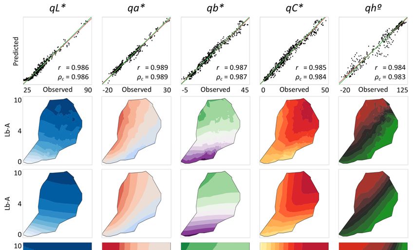
Sensors 2020, 20, 3938                                                                             3 of 15

the relationships between input and output data. This is done by creating intermediary transformation
layers that calculate both the linear and nonlinear relationships between inputs and outputs [21].
Hence, ANN has the ability to capture patterns between data even in non-linear, complex systems [22].
Moreover, its versatility and model-free approach allows the modeling of underlying processes without
restrictive assumptions [23]. In plant research, modeling with neural networks has been successfully
used in a wide range of applications, including optimizing growth media [24,25], classifying cell
wall architecture [26], identifying diseases [27,28], analyzing biophysical properties [29], forecasting
pH and electrical conductivity [30,31], evaluating post-harvest changes and product quality [32–34],
and characterizing and authenticating plant products [35]. Because of the unknown extent of spectral
interference between the two pigments, an ANN appears to be a convenient method for modeling
CMQ coordinates, using chlorophyll and anthocyanin content as input parameters and qL*, qa*, and
qb* values as output parameters.

2. Materials and Methods
     To predict CMQ from the concentration of pigments, four models were developed and tested
on lettuce because its leaves can contain highly variable concentrations of both chlorophylls and
anthocyanins. The best-performing model was subsequently applied to samples from additional plant
species in order to verify that the model can also be used on other herbaceous leaves similar to lettuce.

2.1. Plant Material and Datasets
     Lettuce plants of varying color were grown in a greenhouse or in an open field. Evaluations of leaf
color and quantifications of pigments were performed on 604 samples from ca. 30–60-day-old plants
(primary dataset, Additional file 1 in Supplementary Materials). Because the objective of this study was
to develop the CMQ model for photosynthetically active leaves, only leaves containing chlorophylls
were investigated. Separately, the contents of pigments and leaf color were determined on another
batch of 129 samples (ancillary dataset, Additional file 2 in Supplementary Materials) that comprised
lettuce, leafy vegetables and other plant species (collected from nature). This set included also a few
yellow-, almost white-, and orange-colored leaves, plus flower bracts and petals that were used to
assess the performance and the limitations of the tested models outside of their original scope. Samples
did not have any obvious blemishes, substantial wax deposit, trichomes, or other visible features that
could affect their color. A thin layer of epicuticular wax or minor trichomes on five samples from the
ancillary dataset were removed by gently rubbing their surface with tissue paper. These samples were
not outliers in any of the analyzed parameters, therefore they were kept in the dataset. The common
and scientific names of plant species were used according to The PLANTS Database [36].

2.2. Quantification of Pigments and Measuring Leaf Color
     The content of chlorophylls and anthocyanins was determined on leaves using SPAD-502 (Konica
Minolta Sensing Inc., Tokyo, Japan) and ACM-200 plus (Opti-Sciences, Hudson, New Hampshire, USA)
meters. These devices use light transmittance to provide good in situ estimates of relative contents of
the two pigments [37,38]. The content of chlorophylls was measured in SPAD units, while the content of
anthocyanins was measured in anthocyanins content index (ACI) units. Measurements of chlorophylls
and anthocyanins were taken at antipodal points on adaxial and abaxial leaf surfaces and averaged for
each pigment. Measurements of color were performed using RM200QC spectrocolorimeter (X-Rite,
Grand Rapids, Michigan, USA) on the same adaxial and abaxial leaf areas as those used for evaluations
of chlorophylls and anthocyanins. All measurements of color were done with the D65/10◦ setting
that represents noon daylight with a 10◦ wide view standard observer. SPAD and ACI units were
transformed prior to statistical analyses to improve normality of data distribution. For SPAD data,
the best results were achieved using square root transformation, and thus the chlorophylls units are
shown as ‘SR-S’ (square root of SPAD). For ACI data, the best results were achieved using logarithmic
transformation. To obtain a similar range of transformed data for both pigments, the binary logarithm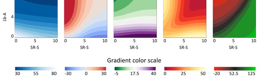
Sensors 2020, 20, 3938                                                                              4 of 15

was applied to transform the ACI values. The transformed anthocyanin units are shown as ‘Lb-A’
(binary logarithm of ACI). To avoid the problem with ‘wraparound’ (crossing 360◦ ) when performing
statistical analyses on hue angles (e.g., the mean of 350◦ and 16◦ is 3◦ , not 183◦ ), the angles between
180◦ and 360◦ were transformed by subtracting 360◦ , thus converting the hue scale to the −180◦ to 180◦
range. The threshold of 180◦ was selected because there were no leaves with h◦ at this range (the hue
of cyan, teal or blue is rare in leaves). Thus, a value of, e.g., 345◦ (purple hue) would be entered into
statistical analyses as −15◦ . The −180◦ to 180◦ scale was used in all statistical analyses, tables and
figures; however, for consistency with CIELab color space, the hue angles were converted back to the
original 0◦ to 360◦ scale when described in the text.

2.3. Parametric Models for Predicting CMQ Coordinates
      The parametric models for predicting CMQ coordinates from chlorophyll and anthocyanin
content were based on three methodologies: full factorial, quadratic polynomial and response surface.
In order to develop respective models and to evaluate their performance, the primary dataset with
measurements taken on 604 lettuce leaves was randomly split into the training and testing datasets.
Approximately 80% of the data (from 480 leaves) were used for developing models (training dataset)
while the remaining ~20% of the data (from 124 leaves) were used to evaluate the quality of the models
(testing dataset). The performance of the models was compared using the coefficient of determination
(R2 ) and the root mean square error (RMSE) calculated between the predicted (modeled) and the
observed color coordinates.

2.4. ANN Models for Predicting CMQ Coordinates
     The primary dataset consisting of data collected from 604 lettuce leaves was used also for the
development and evaluation of models based on ANN. An ANN consists of three types of layers,
namely, input (initial data), hidden (computational) and output (results). Before an ANN can be used
to map the relationship between input (pigments) and output (CMQ coordinates) data, it needs to
be trained to do that. The training process was performed on the training set (data from 480 leaves)
using the input layer consisting of two nodes (SR-S and Lb-A values) and the output layer consisting
from three nodes (qL*, qa* and qb*). The optimum number of hidden nodes in the hidden layer was
determined through the K-fold (K = 10) cross-validation approach that can both gauge the quality
of the particular ANN model and identify instances when over-fitting of the model has occurred.
With K = 10, the training dataset was split into two datasets in a 9:1 ratio. The larger dataset with data
collected from 432 lettuce leaves was used to train ANN, while the smaller dataset (validation set)
with data from 48 lettuce leaves was used to validate the ANN models. Splitting of the dataset and
the cross-validation procedure were performed 20 times for the number of hidden nodes from 1 to
25 (500 runs in total), and the average of the 20 results was used for comparing the performance of
ANN models. The most appropriate number of hidden nodes was identified through minimizing the
negative log-likelihood statistics of the validation set. Because multiple responses (qL*, qa* and qb*)
were predicted using the same ANN model, separate log-likelihoods were computed for each response
(each color coordinate), and the overall log-likelihood for all the responses was calculated by adding
the log-likelihoods of the individual responses [39]. The hyperbolic tangent (TanH) was used as the
transfer function for the hidden layer of nodes, with automated, behind the scenes optimization of the
penalty parameters [39]. Because the log-likelihood statistics indicated that the optimum number of
nodes in the hidden layer was three, all subsequent analyses used the ANN model with two nodes
(SR-S and Lb-A) in the input layer, three nodes in the hidden layer, and three nodes (qL*, qa* and qb*) in
the output layer (Figure 1).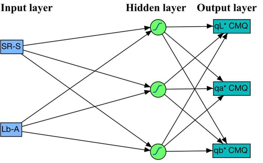
Sensors 2020, 20, 3938 5 of 15
Sensors 2020, 20, x 5 of 15
Figure1.1.Schematic
Figure Schematicstructure
structureofofthe
theselected
selectedartificial
artificialneural
neuralnetwork.
network.TheTheinput
inputlayer
layerhas
hastwotwonodes
nodes
(SR-S and Lb-A), the hidden layer has three nodes, and the output layer (response)
(SR-S and Lb-A), the hidden layer has three nodes, and the output layer (response) has three nodes has three nodes
(qL*,qa*
(qL*, qa*and
and qb*).
qb*). The
The hyperbolic
hyperbolic tangent
tangent (TanH)
(TanH) waswas
usedused astransfer
as the the transfer function
function for thefor the hidden
hidden layer
oflayer of nodes.
nodes.
2.5.
2.5.Calculating
CalculatingCMQ
CMQCoordinates
Coordinatesfrom
fromthe
theContent
ContentofofPigments
Pigments
Because
BecausethetheANN
ANN model
model performed
performed thethe
bestbest
of the
of four models
the four whenwhen
models three three
color coordinates were
color coordinates
considered (Table 1),
were considered only1),
(Table this
onlymodelthis was used
model wasinused
the subsequent analyses.
in the subsequent To understand
analyses. how CMQ
To understand how
color changes with varying levels of both pigments, the ANN model was applied
CMQ color changes with varying levels of both pigments, the ANN model was applied to predict to predict qL*, qa* and
qb* coordinates
qL*, qa* and qb* for all possible combinations
coordinates of SR-S
for all possible (chlorophylls)
combinations ofand
SR-SLb-A (anthocyanins)
(chlorophylls) andvalues
Lb-A
detected in testedvalues
(anthocyanins) plant species
detected(Additional files 1species
in tested plant and 2 in Supplementary
(Additional files 1Materials). These models
and 2 in Supplementary
provide information
Materials). aboutprovide
These models the gamut of qL*, qa*,about
information qb*, qC*
theand
gamutqh◦ofvalues thatqb*,
qL*, qa*, canqC*
be and
expected for each
qh° values that
pigment individually,
can be expected for as well
each as for allindividually,
pigment their combinations.
as well Correlations
as for all theirbetween the modeled
combinations. and the
Correlations
observed
between CMQ coordinates
the modeled andwerethe calculated
observed using
CMQthe Pearson correlation
coordinates coefficient
were calculated (r). Though
using the Pearsonthe
Pearson correlation coefficient provides good information about the closeness
correlation coefficient (r). Though the Pearson correlation coefficient provides good information of data to the best-fitting
line,
aboutit does not take into
the closeness consideration
of data how the best-fitting
to the best-fitting line, it does line conforms
not take intotoconsideration
the identity line. howTherefore,
the best-
Lin’s concordance coefficient (ρ ), which combines both the closeness of the data and
fitting line conforms to the identity line. Therefore, Lin’s concordance coefficient (ρc), which combines
c the conformance
toboth
the the
identity line [40],
closeness of thewas also
data and calculated.
the conformance to the identity line [40], was also calculated.
2.6. Table Performance
1. the
Testing ANN Modelof parametric and Species
on Other Plant empirical models in predicting coordinates of conceptual
midpoint quasi-color (CMQ).
Though the CMQ model was developed using lettuce leaves, for its broad application on
Model
herbaceous Training Setthat
leaves it is desirable (480 Samples)
the model also provides accurate Testing Setestimates
(124 Samples)
of quasi-color
R 2 RMSE R 2 RMSEon lettuce
coordinates for other plant species. To investigate how well the color model developed
leaves works onqL*otherqa* plant qb*species,
qL* comparisons
qa* qb* between
qL* the
qa* predicted
qb* and the
qL* qa* observed
qb*
coordinates
Full factorialwere0.945
performed
0.844 on data from
0.917 2.37 the ancillary
2.72 3.04 dataset
0.963 (Additional
0.857 0.913 file2.31
2 in Supplementary
2.65 3.31
Quadratic This dataset includes data from leafy vegetables and other, mostly herbaceous plant
Materials). 0.962 0.957 0.971 2.00 1.73 1.84 0.978 0.945 0.965 1.83 1.77 2.13
polynomial
species with
Response thin leaves quite similar to lettuce. The ancillary dataset is not intended to provide
0.970 0.964 0.972 1.76 1.58 1.82 0.982 0.950 0.965 1.69 1.66 2.15
exhaustive
surface information about leaf color for all included species; rather, it holds data about the
Artificial neural
common leaf colors
0.969of these
0.979 species.
0.974 This
1.81 dataset
1.23 also
1.71 contains
0.981 a0.979
few samples
0.971 that
1.71 were
1.08 noticeably
1.91
network
very 2different from healthy lettuce leaves, such as yellow-, almost white-, and orange-colored leaves,
R : coefficient of determination. RMSE: root mean square error. qL*, qa*, qb*: CIELab color space coordinates
thickforleaves,
CMQ. colored flower bracts, and white flower petals. These extra samples were included in the
dataset to assess the limitations of the model outside of its original scope. To evaluate the
performance
2.6. Testing the of the Model
ANN modelon onOther
samples
PlantinSpecies
the ancillary dataset, differences between the modeled and
the observed coordinates, as well as overall difference in color ( ∆ = √∆ + ∆ + ∆ ), were
Though the CMQ model was developed using lettuce leaves, for its broad application on
calculated.
herbaceous leaves it is desirable that the model also provides accurate estimates of quasi-color
coordinates for other plant species. To investigate how well the color model developed on lettuce
2.7. Statistical Analyses
leaves works on other plant species, comparisons between the predicted and the observed coordinates
All statistical
were performed onanalyses
data from were
theperformed using JMP
ancillary dataset softwarefile
(Additional v. 14.2.0 (SAS Institute, Cary,
2 in Supplementary North
Materials).
Carolina, USA) and Microsoft Excel for Mac v. 16.16.10 (Microsoft, Redmond, Washington, USA).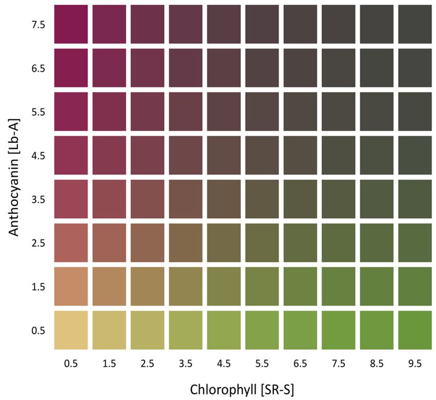
Sensors 2020, 20, 3938                                                                               6 of 15

This dataset includes data from leafy vegetables and other, mostly herbaceous plant species with thin
leaves quite similar to lettuce. The ancillary dataset is not intended to provide exhaustive information
about leaf color for all included species; rather, it holds data about the common leaf colors of these
species. This dataset also contains a few samples that were noticeably very different from healthy lettuce
leaves, such as yellow-, almost white-, and orange-colored leaves, thick leaves, colored flower bracts,
and white flower petals. These extra samples were included in the dataset to assess the limitations of
the model outside of its original scope. To evaluate the performance of the model on samples in the
ancillary dataset, differences
                            √ between the modeled and the observed coordinates, as well as overall
difference in color (∆E = ∆L2 + ∆a2 + ∆b2 ), were calculated.

2.7. Statistical Analyses
   All statistical analyses were performed using JMP software v. 14.2.0 (SAS Institute, Cary, NC,
USA) and Microsoft Excel for Mac v. 16.16.10 (Microsoft, Redmond, WA, USA).

3. Results and Discussion
     A total of 733 samples from 86 plant species were analyzed for the content of chlorophylls and
anthocyanins, and their color. The primary dataset comprised 604 leaf samples from lettuce only, while
the more diverse, ancillary dataset comprised 129 samples from 86 species. The primary dataset was
used to test all models and to select the best model for predicting CMQ coordinates, while the ancillary
dataset was employed to confirm that the model developed on lettuce leaves also provides accurate
results for herbaceous leaves from other plant species.

3.1. Content of Pigments in Lettuce Leaves, Leaf Color and Comparison of Models to Predict CMQ Coordinates
      The content of chlorophylls in the analyzed lettuce leaves ranged from 0 to 8.6 SR-S units, with
the mean value of 5.8 (Additional file 1 in Supplementary Materials). The content of anthocyanins
was in the range from 0.1 to 7.8 Lb-A units, with the mean of 3.6. The qL* ranged from 25.5 to 86
(mean = 41), qa* from −19.7 to 29.1 (mean = −2.8) and qb* from −4.4 to 43.8 (mean = 15.7). Significant
differences were observed between colors on the adaxial and abaxial surfaces of the same leaves,
with lower values of L*, b*, C* and h◦ , but higher values of a*, on adaxial surfaces. On average, the
difference in color of the two surfaces was ∆EDB = 10.3 (Additional file 3 in Supplementary Materials).
The largest difference (∆EDB = 46.4) was detected on lettuce leaves with a very dark red adaxial surface
                                                ◦
(L∗D = 26.2, a∗D = 8, b∗D = −9.9, C∗D = 12.7, hD = 309) but a green abaxial surface (L∗B = 44, a∗B = −12,
                       ◦
b∗B = 28, C∗B = 30.5, hB = 113). These data indicate that associating the content of pigments with color
on only one of the leaf surfaces does not provide complete information and is not suitable for modeling.
      The performance of the ANN model with three hidden layers was compared to the use of three
parametric models on the primary dataset (604 lettuce leaves). On the testing set (124 samples),
the highest R2 and the lowest RMSE values for qa* (0.979 and 1.08, respectively) and qb* (0.971 and 1.91,
respectively) were achieved using the ANN model (Table 1). When the values for qL* coordinate were
considered, the response surface model slightly outperformed the ANN model (R2 of 0.982 versus
0.981, and RMSE of 1.69 versus 1.71). Overall, the best match between the modeled and observed
coordinates of the CMQ were found using the ANN model, followed by the response surface and
quadratic polynomial models. A highly similar pattern was observed in data from the training set
(480 samples). These results indicate that the ANN model provides the most accurate estimates of
CMQ coordinates based on the concentrations of chlorophylls and anthocyanins in lettuce leaves.
Conceivably, this outcome is a result of the ANN model being able to better capture the degree of
spectral inference between pigments than the three tested parametric approaches. The superiority
of ANN over response surface in capturing non-linear behavior was previously reported in several
other [25,29,41,42], but not all [43], evaluated systems.
Sensors 2020, 20, x 7 of 15
R2: coefficient of determination.
Sensors 2020, 20, 3938 7 of 15
RMSE: root mean square error.
3.2. Modeling the Gamut of CMQ
qL*, Coordinates
qa*, qb*: CIELab color space coordinates for CMQ.
Because the ANN
3.2. Modeling model
the Gamut performed
of CMQ better than the parametric models, only this model was used
Coordinates
in the subsequent analyses. The analysis of CMQ coordinates in the data from 604 lettuce leaves
Because the ANN model performed better than the parametric models, only this model was used
(primary dataset,
in the Additional
subsequent fileThe
analyses. 1 inanalysis
Supplementary Materials) in
of CMQ coordinates revealed
the dataa from
strong association
604 between
lettuce leaves
the contents pigments and qL*, qa* and qb*.
(primary dataset, Additional file 1 in Supplementary Materials) revealed a strong association and
of plant The linear correlation between expected
observed values
between thewas 0.986offor
contents plantqL*,pigments
0.989 for andqa*qL*,
andqa*0.987
and qb*. qb* linear
forThe (Figure 2, top row).
correlation Chromaticity
between expected and
hue angle also showed a highly significant (p < 0.0001, n = 604) linear correlation between expected
and observed values was 0.986 for qL*, 0.989 for qa* and 0.987 for qb* (Figure 2, top row). Chromaticity
and hue values
and observed (r =showed
angle also 0.985 for a highly
qC*, andsignificant
0.984 for (P qh ◦ ). ThenLin’s
< 0.0001, = 604) linear correlation
concordance between
coefficient ranged
expected and observed values (r = 0.985 for qC*, and 0.984 for qh°). The Lin’s
from ρc 0.983 to 0.989, demonstrating not only that correlations were high, but that the values wereconcordance coefficient
ranged from ρc 0.983 to 0.989, demonstrating not only that correlations were high, but that the values
close to identity lines.
were close to identity lines.
Figure 2. Observed and predicted coordinates of qL*, qa*, qb*, qC* and qh° for conceptual midpoint
Figure 2. Observed and predicted coordinates of qL*, qa*, qb*, qC* and qh◦ for conceptual midpoint
quasi-color (CMQ) assessed on 604 samples of cultivated lettuce. Top row shows linear correlations
quasi-color (CMQ) assessed on 604 samples of cultivated lettuce. Top row shows linear correlations
between observed and predicted values. Predicted values were calculated from contents of
between observed and predicted values. Predicted values were calculated from contents of chlorophylls
chlorophylls (SR-S values) and anthocyanins (Lb-A values) using an artificial neural network (ANN).
(SR-S values) and anthocyanins
The red lines indicate the best(Lb-A
linear values) using
fit between an artificial
observed neuralvalues,
and predicted network (ANN).
while Thelines
the green red lines
indicatearethe best lines
identity linear
(x fit between
= y). observed
All correlation and predicted
coefficients were highlyvalues, while
significant (P the green
< 0.0001, n =lines
604). are identity
Scales
lines (xof=x-axis
y). All correlation
and y-axis are coefficients
identical for were highly
individual CMQ significant (p < thus
coordinates, for n
0.0001, = 604).
clarity Scales
of the of x-axis
figure only and
y-axis are identical for individual CMQ coordinates, thus for clarity of the figure only the range on the
x-axes are indicated. Rows two to four show 3D presentations of values for each CMQ coordinate. Row
two shows observed values from 604 lettuce samples, row three shows predicted values using an ANN,
and row four shows predicted values for the extrapolated range of pigments (those combinations not
present in the original samples). Note that rows two and three show values for the range of chlorophylls
and anthocyanins detected in lettuce leaves only, while row four shows also values extrapolated outside
of this range, but found in other tested plant species. Color gradients for CMQ coordinates in rows two
to four are indicated at the bottom of the figure.Sensors 2020, 20, 3938 8 of 15
The additional rows in Figure 2 show 3D presentations of observed CMQ values from 604 lettuce
samples (second row), predicted CMQ values using the ANN model (third row), and predicted CMQ
values for the range of pigments found in all tested plants (fourth row). This range of pigments
includes also hypothetical combinations of chlorophylls and anthocyanins that were not actually
detected in the analyzed samples. Modeled values of qL* decreased with the increasing content of both
pigments, while the qa* and qb* values were affected more by the relative content of chlorophylls and
anthocyanins in leaves (Figure 2). The values of all three coordinates, however, were affected more by
Lb-A than SR-S, with the relative impact of the independent variables on qL* being 90.6% and 5.6%,
on qa* 60.4% and 36.1%, and on qb* 83.6% and 12.8%, respectively. The highest vividness of quasi-colors
(largest qC*) was detected in leaves with high contents of either pigment alone. If both pigments were
present in the leaf together, particularly at very high contents, the quasi-color became duller (Figure 3,
upper right corner). When leaves contained only a high content of anthocyanins, the modeled hue
angle was in the purple–red range (~340◦ ) (Figure 3, upper left corner), while for leaves that contained
only a high content of chlorophylls, the modeled hue angle was in the green range (~125◦ ) (Figure 3,
lower right corner). For leaves with identical coloration on adaxial and abaxial surfaces, the qL*, qa*
and qb* coordinates predicted for the CMQ are the same as the L*, a* and b* coordinates predicted for
each of the two leaf surfaces. The ANN formulas for the CMQ model are:
qL* = 76.8278 − 23.3637 * H1 + 0.6636 * H2 −24.9085 * H3 (1)
qa* = −13.0326 + 24.3295 * H1+ 34.7418 * H2 + 22.0398 * H3 (2)
qb* = 28.5284 − 34.0210 * H1 − 5.4716 * H2 + 0.7791 * H3 (3)
where,
H1 = Tanh [0.5 * (−1.0617 + 0.0311 * SR-S + 0.6420 * Lb-A)] (4)
H2 = Tanh [0.5 * (1.4045 − 0.5334 * SR-S − 0.0241 * Lb-A)] (5)
H3 = Tanh [0.5 * (−0.1777 + 0.3507 * SR-S + 0.9401 * Lb-A)] (6)
Sensors 2020, 20, x 9 of 15
Figure 3. Predictive modeling of a leaf conceptual midpoint quasi-color (CMQ) from the content of
Figure 3. Predictive modeling of a leaf conceptual midpoint quasi-color (CMQ) from the content of
chlorophylls and anthocyanins. CMQ values were predicted using the artificial neural network
chlorophylls and
(ANN)anthocyanins. CMQ
approach. The results arevalues were
shown for the predicted
approximate using
range ofthe artificial
pigments neural
content network (ANN)
that was
approach. Thefound in theare
results analyzed
shown set of
forleaves
the (Additional
approximatefiles 1 range
and 2 inof
Supplementary
pigments Materials). Whenwas
content that the found in the
colorations of a leaf’s adaxial and abaxial surfaces are identical, the qL*, qa* and qb* coordinates
analyzed set of leaves (Additional files 1 and 2 in Supplementary Materials). When the colorations of a
predicted for the CMQ are the same as the L*, a* and b* coordinates predicted for each of the two leaf
and abaxial surfaces are identical, the qL*, qa* and qb* coordinates predicted for the CMQ
leaf’s adaxial surfaces.
are the same as the L*, a* and b* coordinates predicted for each of the two leaf surfaces.
3.3. Performance of the ANN Model on Herbaceous Leaves
Lettuce was used to develop the ANN model because of the high variability in its leaf color and
concentration of pigments. However, for a broad application on herbaceous leaves, the model also
needs to provide reliable results for other plant species with similar leaf characteristics. To test how
the CMQ model that was developed for cultivated lettuce applies to other plants, further assessments
were performed on 129 additional samples from other species and cultivars that showed a wider
range in their contents of both chlorophylls (SR-S from 0 to 9.7) and anthocyanins (Lb-A from 0 to
8.0) (ancillary dataset, Additional file 2 in Supplementary Materials) than was observed for theSensors 2020, 20, 3938 9 of 15
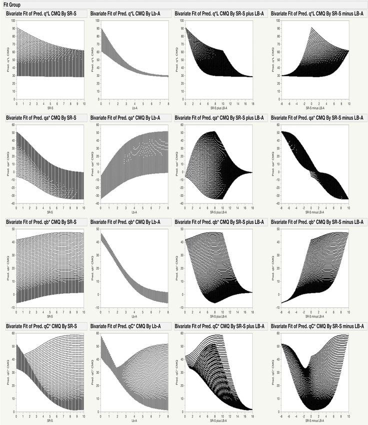
The gamut of possible qL*, qa*, qb*, qC* and qh◦ values, and their distribution for each pigment
individually, but also for their combination, is shown in Figure 4. For example, the values of qb*
(Figure 4, third row) for the CMQ can be in the wide range of ~0 to ~45 when the SR-S is 5.0. However,
the range of possible qb* values for the CMQ is much narrower for any particular content of Lb-A;
e.g., only from ~4 to ~10 for Lb-A of 4.0. The figure also shows how the values of each coordinate
change when the combined content of both pigments increases (‘plus values’ in the third column),
or when the difference in the content of pigments changes (‘minus values’ in the fourth column).
Based on the ANN model, the only possible values of qL*, qa*, qb*, qC* and qh◦ for the CMQ are those
shown in Figure 4.
3.3. Performance of the ANN Model on Herbaceous Leaves
Lettuce was used to develop the ANN model because of the high variability in its leaf color and
concentration of pigments. However, for a broad application on herbaceous leaves, the model also
needs to provide reliable results for other plant species with similar leaf characteristics. To test how the
CMQ model that was developed for cultivated lettuce applies to other plants, further assessments
were performed on 129 additional samples from other species and cultivars that showed a wider
range in their contents of both chlorophylls (SR-S from 0 to 9.7) and anthocyanins (Lb-A from 0 to 8.0)
(ancillary dataset, Additional file 2 in Supplementary Materials) than was observed for the analyzed
lettuces (primary dataset, Additional file 1 in Supplementary Materials). The differences between
the predicted and observed values for samples in this dataset were larger than for samples in the
primary dataset. The values of ∆qL ranged from −11.6 to 16.0, of ∆qa from −5.5 to 15.0, and of ∆qb
from −36.1 to 28.8 (Additional files 2 and 4 in Supplementary Materials). When all the coordinates
were considered, the largest differences (∆qE) were found for samples with almost no chlorophyll
when they visually appeared white (flower petal of daisy ∆qE = 36.4), bright red (bract of poinsettia
∆qE = 33.7), intensive yellow (dying leaf of bear’s breech ∆qE = 27.1) or were thick and/or dense
(camellia ∆qE = 17.5) (Additional files 2 and 4 in Supplementary Materials). The model worked well for
all tested leafy vegetables (chard, cultivated endive, common dandelion, Lewiston cornsalad, pak choi,
radicchio, rocket salad, spinach, tender green and treviso) regardless of their color, and also on other
plant species with comparable leaf characteristics. The test indicates, however, that the ANN-based
CMQ model, which was developed on thin, photosynthetically active, herbaceous leaves of lettuce,
may be less reliable for predicting the quasi-color values of leaves with substantially different structures,
thicknesses, dry masses, pHs (which can change anthocyanin color) and pigment compositions, or for
leaves that are covered with wax, trichomes or other features modifying the visual appearance of
their color.Sensors 2020, 20, 3938 10 of 15
Sensors 2020, 20, x 10 of 15
Figure 4. Visualization of the relationship between the predicted values of qL*, qa*, qb*, qC* and qh°
Figure 4. Visualization of the relationship between the predicted values of qL*, qa*, qb*, qC* and qh◦
coordinates for CMQ, and the range of chlorophylls and anthocyanins content detected in analyzed
coordinates for CMQ, and the range of chlorophylls and anthocyanins content detected in analyzed
plants. Predicted values of qL*, qa*, qb*, qC* and qh° coordinates (rows) were plotted against values of
plants. Predicted values
SR-S, Lb-A, SR-S qL*, qa*,
plusofLb-A, and qb*,
SR-SqC*minus qh◦ coordinates
andLb-A (columns), in(rows) were
order to plotted
visualize theagainst values of
relationship
SR-S,between
Lb-A, SR-S plus Lb-A, and SR-S minus Lb-A (columns), in order to visualize the
pigments content and CMQ coordinates. These graphs show how each of the pigments and relationship
between pigments content and CMQ coordinates. These graphs show how each of the pigments and
their combinations affect qL*, qa*, qb*, qC* and qh◦ values. For example, when the SR-S value is equal to
5, the predicted qL* values will be approximately in the range of 30–70 (upper left panel).Sensors 2020, 20, 3938 11 of 15
From the set of tested samples, the CMQ model predicted the darkest quasi-color (lowest qL*
value) for mondo grass (Ophiopogon planiscapus Nakai) cv. Nigrescens, which contains large quantities
of both chlorophylls (SR-S of 9.7) and anthocyanins (Lb-A of 7.5). The modeling results (qL* = 28.7,
qa* = −0.9 and qb* = 1.7) matched well with the empirical values found in this (qL* = 25.8, qa* = −1.6 and
qb* = 3.2) (Additional file 2 in Supplementary Materials) and earlier [44] studies (qL* = 29, qa* = −1.9
and qb* = 3.3 were calculated from the values of L*, C* and h◦ reported for both leaf surfaces). It was
previously shown that the blackish color of this cultivar was caused by abundant contents of both
chlorophylls and anthocyanins, but not carotenoids [44]. Results of the present study also show that
estimating the content of chlorophylls and anthocyanins from the visual appearance of leaves may be
problematic when both pigments are present in the samples simultaneously, because the perceived
‘greenness’ or ‘redness’ of a leaf is affected not only by the content, but also by the ratio of the two
pigments. For example, when both anthocyanins and chlorophylls were present in lettuce leaves in
detectable quantities, no correlation was found between the chlorophyll content and values of a* or
b* [45]. Such results accentuate the conclusions of the present study, regarding the combined effect of
both pigments on the CIELab color coordinates of a leaf (Figures 2–4). In addition, modeling of the
CMQ coordinates shows that when both chlorophylls and anthocyanins are present in the same leaf
tissue, a correlation between the content of chlorophylls and the qL*, qa* or qb* coordinates (or derived
qC*, qh◦ ) may not be detected because of the spectral interference between the two pigments. However,
there appears to be a strong relationship between the content of anthocyanins and color coordinates
(Figure 4, second column), particularly with qL* and qb*, though even these may be affected to a certain
extent by the presence of chlorophylls.
3.4. Dorsiventral Distribution of Pigments
Current analysis and modeling show that highly different colors of leaves may result from similar
contents of pigments but their different dorsiventral distribution. For example, leaf samples LS-385
and LS-101 (Additional file 1 in Supplementary Materials) have similar contents of chlorophylls (SR-S
of 5.4 for both) and anthocyanins (Lb-A of 3.7 and 3.9, respectively). Therefore, they also have similar
qL* (37.1 and 36.1), qa* (1.4 and 2.3) and qb* (11.5 and 10.2) coordinates, predicted for CMQ. However,
while LS-385 has a fairly similar color on both leaf surfaces (adaxial LD * = 33.9, aD * = 1.7 and bD * = 8.3;
abaxial LB * = 37.0, aB * = 2.6, bB * = 10.1; ∆EDB = 3.7), the color of the leaf surfaces is highly different
for LS-101 (adaxial LD * = 23.1, aD * = 8.1 and bD * = 5.2; abaxial LB * = 50.3, aB * = −4.1, bB * = 16.3;
∆EDB = 31.8). Leaf color modeling approaches that consider only one, usually adaxial, surface of the
leaves, or assume that both surfaces have a similar color, would indicate that the color of either LS-385
or LS-101 is in discrepancy with the content of pigments. The CMQ approach allows, however, for such
differences in colors. Assuming that the actual color for one of the leaf surfaces (e.g., adaxial) can
be obtained, it is possible to estimate the unknown color of the abaxial surface by subtracting the
color coordinates of the adaxial surface from the CMQ coordinates (multiplied by two, because they
correspond to the mean of both surfaces), modeled from the content of pigments. In this example,
the expected coordinates for LS-385 (qLB * = 40.2, qaB * = 1.0 and qbB * = 14.6) and LS-101 (qLB * = 49.2,
qaB * = −3.6 and qbB * = 15.2) are in the range of the actual values measured on the abaxial surfaces,
confirming that highly different colors may be observed on leaves with similar contents of pigments but
different dorsiventral distributions. Such dorsiventral distribution of pigments needs to be taken into
consideration when modeling [6–10] or monitoring [46,47] leaf colors and their changes, particularly
as regards plant species or cultivars with high contents of both pigments.
3.5. Application of CMQ in Plant Research
Due to spectral inference between pigments [4], the concentration of chlorophylls and anthocyanins
cannot be accurately estimated from fruit [11] or leaf [4] color when they co-occur within the same
tissue in high enough quantities. A limited approximation of the concentration range for anthocyanins
can be deduced from the CMQ coordinates calculated from the abaxial and adaxial leaf colors (Figure 4,Sensors 2020, 20, 3938 12 of 15
second column). However, no reliable estimate is possible for most of the concentrations of chlorophylls
(Figure 4, first column), because chlorophylls affect the change in color coordinates relatively less
significantly than anthocyanins do (~6:91 ratio for qL*, ~36:60 ratio for qa* and ~13:84 ration for qb*).
The CMQ approach could be used to model virtual [6–10] colors of leaves [12] when studying
the mechanism of color change [13,48]. The approach could also be used to model ‘customized’ leaf
colors [49] in environments where both leaf surfaces are not observable. For example, when the
abaxial color of prostrate leaves cannot be seen on plants grown in controlled-environment agriculture
(indoor farms), but knowing that color is important to the industry, concentrations of pigments for a
particular cultivar could be modeled [10] from nutrition [50], temperature [19], light [51,52] and other
environmental data, while the adaxial color of leaves can be measured with overhead sensors. CMQ
coordinates (calculated from modeled concentrations of pigments using formulas provided in this
study) can then be applied, together with adaxial color data, to estimate abaxial leaf color.
4. Conclusions
This work provides the proof of concept for the use of CMQ in plant research. The ANN model
outperformed the full factorial, quadratic polynomial and response surface models for predicting the
qa* and qb* coordinates of CMQ, and was only marginally worse than the response surface model in
predicting qL* values. These results suggest that the ANN model surpasses the parametric models in
capturing spectral inference between pigments. Thus, the ANN-based CMQ model can be used to
test the distribution of color in the bifacial leaves of lettuce and other leafy vegetables, as well as its
diversity and association with pigments. This approach may be particularly helpful when modeling
the color of leaves with large dorsiventral differences. In such leaves, combining the color coordinates
from both surfaces allows for finer association with the content of chlorophylls and anthocyanins
than does use of color data from a single surface only. However, it may be necessary to develop
specific models for other types of leaves that do not conform to the lettuce-based model. Though CMQ
coordinates per se do not indicate the actual leaf color, these coordinates match well with the content
of pigments in leaf tissue. CMQ coordinates could thus be used, for example, for estimating L*, a* and
b* on an unobservable leaf surface when the content of chlorophylls and anthocyanins is known, and
the color coordinates for one of the surfaces could be measured. For plants with similar coloration
on both leaf surfaces, the CMQ model could be used to directly predict their color from their content
of chlorophylls and anthocyanins. When the colorations of a leaf’s adaxial and abaxial surfaces are
identical, the qL*, qa* and qb* coordinates predicted for CMQ are the same as L*, a* and b* coordinates
predicted for each of the two leaf surfaces.
Supplementary Materials: The following are available online at http://www.mdpi.com/1424-8220/20/14/3938/s1,
Dataset S1: The list of 604 lettuce samples that were used to develop the ANN model of leaf color (primary
dataset). Dataset S2: The list of 129 samples that were used to assess performance of the lettuce-based model of
leaf color developed through ANN approach (ancillary dataset). Figure S3: Distribution of differences between
color coordinates measured on adaxial and abaxial surfaces of 604 lettuce leaves. Figure S4: Distribution of
differences between predicted and observed CMQ coordinates for 129 samples.
Funding: This research received no external funding.
Conflicts of Interest: The author declares no conflict of interest.
References
1. Boldt, J.K.; Meyer, M.H.; Erwin, J.E. Foliar anthocyanins: A horticultural review. Hortic. Rev. 2014, 42,
209–252.
2. Mahlein, A.-K. Plant disease detection by imaging sensors—Parallels and specific demands for precision
agriculture and plant phenotyping. Plant. Dis. 2016, 100, 241–251. [CrossRef] [PubMed]
3. Simko, I.; Jimenez-Berni, J.A.; Sirault, X.R. Phenomic approaches and tools for phytopathologists.
Phytopathology 2017, 107, 6–17. [CrossRef] [PubMed]Sensors 2020, 20, 3938 13 of 15
4. Sims, D.A.; Gamon, J.A. Relationships between leaf pigment content and spectral reflectance across a
wide range of species, leaf structures and developmental stages. Remote Sens. Environ. 2002, 81, 337–354.
[CrossRef]
5. Junker, L.V.; Ensminger, I. Relationship between leaf optical properties, chlorophyll fluorescence and pigment
changes in senescing Acer saccharum leaves. Tree Physiol. 2016, 36, 694–711. [CrossRef] [PubMed]
6. Braitmaier, M.; Diepstraten, J.; Ertl, T. Real-time rendering of seasonal influenced trees. In Proceedings of the
Theory and Practice of Computer Graphics, Bournemouth, UK, 8–10 June 2004; pp. 152–159.
7. Miao, T.; Zhao, C.; Guo, X.; Lu, S. A framework for plant leaf modeling and shading. Math. Comput. Model.
2013, 58, 710–718. [CrossRef]
8. Wang, X.; Zhao, C.; Lu, S.; Guo, X. Survey on modeling and visualization of plant leaf color. In Proceedings of
the Third International Symposium on Plant Growth Modeling, Simulation, Visualization and Applications,
Beijing, China, 9–13 November 2009; pp. 417–424.
9. Yi, W.-L.; He, H.-J.; Wang, L.-P.; Yang, H.-Y. Modeling and simulation of leaf color based on virtual rice.
In Proceedings of the International Conference on Materials, Manufacturing and Mechanical Engineering,
Beijing, China, 30–31 December 2016; pp. 334–343.
10. Zhou, N.; Dong, W.; Mei, X. Realistic simulation of seasonal variant maples. In Proceedings of the Second
International Symposium on Plant Growth Modeling and Applications, Beijing, China, 13–17 November 2006;
pp. 295–301.
11. Lancaster, J.E.; Lister, C.E.; Reay, P.F.; Triggs, C.M. Influence of pigment composition on skin color in a wide
range of fruit and vegetables. J. Am. Soc. Hortic. Sci. 1997, 122, 594–598. [CrossRef]
12. Lu, S.; Wang, L.; He, H.; Guo, X. Visual simulation of cucumber leaf color based on the relative content of
chlorophyll. Trans. Chin. Soc. Agric. Mach. 2014, 45, 250–254.
13. Shen, J.; Zou, Z.; Zhang, X.; Zhou, L.; Wang, Y.; Fang, W.; Zhu, X. Metabolic analyses reveal different
mechanisms of leaf color change in two purple-leaf tea plant (Camellia sinensis L.) cultivars. Hortic. Res. 2018,
5, 7. [CrossRef]
14. Wang, Y.; Wang, D.; Shi, P.; Omasa, K. Estimating rice chlorophyll content and leaf nitrogen concentration
with a digital still color camera under natural light. Plant. Methods. 2014, 10, 36. [CrossRef]
15. Gazula, A.; Kleinhenz, M.D.; Scheerens, J.C.; Ling, P.P. Anthocyanin levels in nine lettuce (Lactuca sativa)
cultivars: Influence of planting date and relations among analytic, instrumented, and visual assessments of
color. HortScience 2007, 42, 232–238. [CrossRef]
16. Gonçalves, B.; Silva, A.P.; Moutinho-Pereira, J.; Bacelar, E.; Rosa, E.; Meyer, A.S. Effect of ripeness and
postharvest storage on the evolution of colour and anthocyanins in cherries (Prunus avium L.). Food Chem.
2007, 103, 976–984.
17. Fairchild, M.D. Color Appearance Models, 3rd ed.; John Wiley & Sons: Chichester, UK, 2013.
18. Simko, I.; Hayes, R.J.; Mou, B.; McCreight, J.D. Lettuce and Spinach. In Yield Gains in Major, U.S. Field Crops;
Smith, S., Diers, B., Specht, J., Carver, B., Eds.; American Society of Agronomy, Crop Science Society of
America, and Soil Science Society of America: Madison, WI, USA, 2014; pp. 53–86.
19. Simko, I.; Hayes, R.J.; Furbank, R.T. Non-destructive phenotyping of lettuce plants in early stages of
development with optical sensors. Front. Plant. Sci. 2016, 7, 1985. [CrossRef] [PubMed]
20. Parisi, G.I.; Kemker, R.; Part, J.L.; Kanan, C.; Wermter, S. Continual lifelong learning with neural networks:
A review. Neural Netw. 2019, 113, 54–71. [CrossRef] [PubMed]
21. Lazarovits, J.; Sindhwani, S.; Tavares, A.J.; Zhang, Y.; Song, F.; Audet, J.; Krieger, J.R.; Syed, A.M.; Stordy, B.;
Chan, W.C. Supervised learning and mass spectrometry predicts the in vivo fate of nanomaterials. ACS Nano
2019, 13, 8023–8034. [CrossRef] [PubMed]
22. Hinton, G.E.; Salakhutdinov, R.R. Reducing the dimensionality of data with neural networks. Science 2006,
313, 504–507. [CrossRef]
23. Zhang, G.; Patuwo, B.E.; Hu, M.Y. Forecasting with artificial neural networks: The state of the art.
Int. J. Forecast. 1998, 14, 35–62. [CrossRef]
24. Arab, M.M.; Yadollahi, A.; Shojaeiyan, A.; Ahmadi, H. Artificial neural network genetic algorithm as powerful
tool to predict and optimize in vitro proliferation mineral medium for G × N15 rootstock. Front. Plant. Sci.
2016, 7, 1526. [CrossRef]Sensors 2020, 20, 3938 14 of 15
25. Mohamed, M.S.; Tan, J.S.; Mohamad, R.; Mokhtar, M.N.; Ariff, A.B. Comparative analyses of response surface
methodology and artificial neural network on medium optimization for Tetraselmis sp. FTC209 grown under
mixotrophic condition. Sci. World J. 2013, 2013, 948940. [CrossRef]
26. McCann, M.C.; Defernez, M.; Urbanowicz, B.R.; Tewari, J.C.; Langewisch, T.; Olek, A.; Wells, B.; Wilson, R.H.;
Carpita, N.C. Neural network analyses of infrared spectra for classifying cell wall architectures. Plant. Physiol.
2007, 143, 1314–1326. [CrossRef]
27. Huang, K.-Y. Application of artificial neural network for detecting Phalaenopsis seedling diseases using
color and texture features. Comput. Electron. Agric. 2007, 57, 3–11. [CrossRef]
28. Toda, Y.; Okura, F. How convolutional neural networks diagnose plant disease. Plant. Phenomics. 2019,
2019, 9237136. [CrossRef]
29. Ghodsvali, A.; Farzaneh, V.; Bakhshabadi, H.; Zare, Z.; Karami, Z.; Mokhtarian, M.; Carvalho, I.S. Screening
of the aerodynamic and biophysical properties of barley malt. Int. Agrophysics. 2016, 30, 457–464. [CrossRef]
30. Ferentinos, K.; Albright, L. Predictive neural network modeling of pH and electrical conductivity in
deep–trough hydroponics. Trans. Asae 2002, 45, 2007. [CrossRef]
31. Moon, T.; Ahn, T.I.; Son, J.E. Forecasting root-zone electrical conductivity of nutrient solutions in
closed-loop soilless cultures via a recurrent neural network using environmental and cultivation information.
Front. Plant. Sci. 2018, 9. [CrossRef] [PubMed]
32. Cavallo, D.P.; Cefola, M.; Pace, B.; Logrieco, A.F.; Attolico, G. Non-destructive automatic quality evaluation
of fresh-cut iceberg lettuce through packaging material. J. Food Eng. 2018, 223, 46–52. [CrossRef]
33. Taghadomi-Saberi, S.; Omid, M.; Emam-Djomeh, Z.; Ahmadi, H. Evaluating the potential of artificial neural
network and neuro-fuzzy techniques for estimating antioxidant activity and anthocyanin content of sweet
cherry during ripening by using image processing. J. Sci. Food Agric. 2014, 94, 95–101. [CrossRef]
34. Wang, Z.-W.; Duan, H.-W.; Hu, C.-Y. Modelling the respiration rate of guava (Psidium guajava L.) fruit using
enzyme kinetics, chemical kinetics and artificial neural network. Eur. Food Res. Technol. 2009, 229, 495–503.
[CrossRef]
35. Gonzalez-Fernandez, I.; Iglesias-Otero, M.; Esteki, M.; Moldes, O.; Mejuto, J.; Simal-Gandara, J. A critical
review on the use of artificial neural networks in olive oil production, characterization and authentication.
Crit. Rev. Food Sci. Nutr. 2019, 59, 1913–1926. [CrossRef]
36. The PLANTS Database. United States Department of Agriculture, Natural Resources Conservation Service,
Washington, D.C. Available online: https://plants.sc.egov.usda.gov (accessed on 14 November 2018).
37. Parry, C.; Blonquist, J.M., Jr.; Bugbee, B. In situ measurement of leaf chlorophyll concentration: Analysis of
the optical/absolute relationship. Plant Cell Environ. 2014, 37, 2508–2520. [CrossRef]
38. van den Berg, A.K.; Perkins, T.D. Nondestructive estimation of anthocyanin content in autumn sugar maple
leaves. HortScience 2005, 40, 685–686. [CrossRef]
39. Gotwalt, C.M. JMP Neural Network Methodology; SAS Institute: Cary, NC, USA, 2012.
40. Lin, L.I.-K. A concordance correlation coefficient to evaluate reproducibility. Biometrics 1989, 255–268.
[CrossRef]
41. Basri, M.; Abd Rahman, R.N.Z.R.; Ebrahimpour, A.; Salleh, A.B.; Gunawan, E.R.; Abd Rahman, M.B.
Comparison of estimation capabilities of response surface methodology (RSM) with artificial neural network
(ANN) in lipase-catalyzed synthesis of palm-based wax ester. BMC Biotechnol. 2007, 7, 53. [CrossRef]
[PubMed]
42. Desai, K.M.; Survase, S.A.; Saudagar, P.S.; Lele, S.; Singhal, R.S. Comparison of artificial neural network
(ANN) and response surface methodology (RSM) in fermentation media optimization: Case study of
fermentative production of scleroglucan. Biochem. Eng. J. 2008, 41, 266–273. [CrossRef]
43. Pakalapati, H.; Arumugasamy, S.K.; Khalid, M. Comparison of response surface methodology and
feedforward neural network modeling for polycaprolactone synthesis using enzymatic polymerization.
Biocatal. Agric. Biotechnol. 2019, 18, 101046. [CrossRef]
44. Hatier, J.-H.B.; Gould, K.S. Black coloration in leaves of Ophiopogon planiscapus ‘Nigrescens’. Leaf optics,
chromaticity, and internal light gradients. Funct. Plant. Biol. 2007, 34, 130–138. [CrossRef]
45. Mampholo, B.M.; Maboko, M.M.; Soundy, P.; Sivakumar, D. Phytochemicals and overall quality of leafy
lettuce (Lactuca sativa L.) varieties grown in closed hydroponic system. J. Food Qual. 2016, 39, 805–815.
[CrossRef]You can also read