MAPPING FOLIAR NUTRITION USING WORLDVIEW-3 AND WORLDVIEW-2 TO ASSESS KOALA HABITAT SUITABILITY - MDPI
←
→
Page content transcription
If your browser does not render page correctly, please read the page content below
remote sensing
Article
Mapping Foliar Nutrition Using WorldView-3 and
WorldView-2 to Assess Koala Habitat Suitability
Huiying Wu 1, * , Noam Levin 1,2 , Leonie Seabrook 1 , Ben Moore 3 and Clive McAlpine 1
 1    School of Earth and Environmental Sciences, The University of Queensland, Brisbane, QLD 4072, Australia;
      l.seabrook@uq.edu.au (L.S.); c.mcalpine@uq.edu.au (C.M.)
 2    Department of Geography, The Hebrew University of Jerusalem, Mount Scopus, Jerusalem 91905, Israel;
      noamlevin@mail.huji.ac.il (N.L.)
 3    Hawkesbury Institute for the Environment, The University of Western Sydney, Locked Bag 1797, Penrith,
      NSW 2751, Australia; b.moore@westernsydney.edu.au (B.M.)
 *    Correspondence: hui.wu@uqconnect.edu.au; Tel.: +86-182-186-71929

 Received: 16 December 2018; Accepted: 17 January 2019; Published: 22 January 2019

 Abstract: Conservation planning and population assessment for widely-distributed, but vulnerable,
 arboreal folivore species demands cost-effective mapping of habitat suitability over large areas.
 This study tested whether multispectral data from WorldView-3 could be used to estimate
 and map foliar digestible nitrogen (DigN), a nutritional measure superior to total nitrogen for
 tannin-rich foliage for the koala (Phascolarctos cinereus). We acquired two WorldView-3 images
 (November 2015) and collected leaf samples from Eucalyptus woodlands in semi-arid eastern Australia.
 Linear regression indicated the normalized difference index using bands “Coastal” and “NIR1” best
 estimated DigN concentration (% dry matter, R2 = 0.70, RMSE = 0.19%). Foliar DigN concentration
 was mapped for multi-species Eucalyptus open woodlands across two landscapes using this index.
 This mapping method was tested on a WorldView-2 image (October 2012) with associated koala
 tracking data (August 2010 to November 2011) from a different landscape of the study region.
 Quantile regression showed significant positive relationship between estimated DigN and occurrence
 of koalas at 0.999 quantile (R2 = 0.63). This study reports the first attempt to use a multispectral
 satellite-derived spectral index for mapping foliar DigN at a landscape-scale (100s km2 ). The mapping
 method can potentially be incorporated in mapping and monitoring koala habitat suitability for
 conservation management.

 Keywords: remote sensing; Eucalyptus; digestible nitrogen; koalas; habitat mapping

1. Introduction
      Mapping and monitoring habitat suitability for threatened species at the landscape and regional
scale (≥ 100s km2 ) is crucial for developing effective conservation management [1–4]. This is especially
important for conserving specialist folivores such as the koala, Phascolarctos cinereus, the distribution of
which at the landscape scale is determined largely by the occurrence of nutrient-rich foliage of food
tree species [5,6]. Koalas are listed as ‘Vulnerable’ in the IUCN red list [7] and are threatened by disease
and habitat destruction and fragmentation. Current published mapping of koala habitat suitability
relies mainly on vegetation community mapping, especially the relative proportion of primary food
tree species [2]. Although the primary food tree species vary in different regional landscapes with
different eucalypt species communities, the more frequent koala use of these primary food tree species
is related to leaf nutritional quality [4,8] which shows spatial variation [9] and could be affected by
water availability and soil fertility [10,11]. Incorporating leaf nutritional information is one of the
suggested enhancements to this method [2] because of the patchy distribution of antifeedant chemistry

Remote Sens. 2019, 11, 215; doi:10.3390/rs11020215                        www.mdpi.com/journal/remotesensing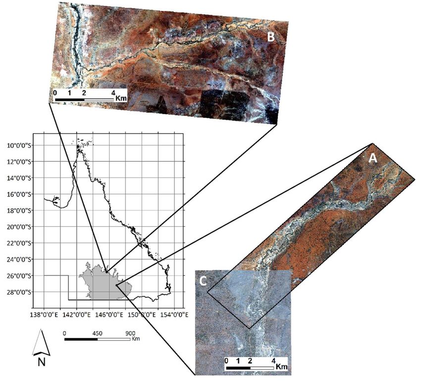
Remote Sens. 2019, 11, 215                                                                           2 of 17

and forage nutrients found in previous studies [9,10]. Koala food selection is a key determinant of tree
use and is influenced by foliar water content, nitrogen, and concentrations of several groups of plant
secondary metabolites (e.g., tannins and formylated phloroglucinol compounds) [8,11]. In the past,
plant nutritional value to herbivores has been estimated using total nitrogen (N) or protein-to-fibre
ratios [12,13]. However, for browse or foliage diets, protein (and hence N) digestibility can be
significantly reduced by tannins. Tannins are widespread plant secondary metabolites which form
insoluble tannin-protein complexes which resist digestion in the mammalian gut. Digestible N (DigN)
concentration can be estimated by an in vitro digestion assay [14] and better reflects the nutritional
value of tannin-rich foods, such as eucalypt foliage, to mammalian folivores. DigN has been shown to
influence koala feeding decisions [10] and breeding success in eucalypt-feeding common brushtail
possums [15]. Because DigN integrates the nutritional information of both attractants and deterrents
to feeding, mapping DigN across an area would be another step forward from mapping attractants
and deterrents individually [16] to meet the need of more specific measured food quality for herbivore
conservation and habitat management.
      Determining foliar quality over large areas using field-sampling and chemical analysis involves
very large sample sizes and is unavoidably expensive [17–19]. Remote sensing applications offer new
opportunities to address this problem by providing proximal data for estimating plant chemistry [20].
An ideal remote sensing data source for mapping foliar DigN would have adequate spatial resolution
to isolate individual tree spectra, an appropriate spectral response to provide sensitive indices and
a relatively lower cost. It is encouraging that foliar DigN was accurately modelled from airborne
hyperspectral data in Australian temperate eucalypt woodlands [19]. However, mapping large
areas with airborne remote sensing is generally more expensive than multispectral satellite remote
sensing [21]. There is a need to find satellite-derived data that have high spatial resolution and can
provide sensitive spectral indices for foliar DigN.
      No studies mapping DigN with satellite remote sensing were found during our literature
search, but a wide range of studies have used satellite-derived data (from WorldView-2, SPOT,
Hyperion, Aster, Sentinel-2, and IKONOS) to map N in crops and trees [20,22–26]. Several suitable
spectral indices have been found for mapping N using satellite-derived multispectral data such as
Aster [21], Sentinel-2 [26], and WorldView-2 [20]. Testing potential spectral indices may identify
appropriate indices for estimating and mapping DigN. Yet the requirement of high spatial resolution
for mapping foliar DigN in individual trees narrows the range of suitable sensors. For example,
many eucalypt canopies [27] are smaller than the spatial resolution of Hyperion (30 m), Aster (15 m),
and SPOT (10 m). On the other hand, DigN results from the interactions of N, tannins and fibre
in leaves, which have important absorption features in the shortwave infrared (SWIR) region [19].
Previously, most high-resolution satellite-borne sensors did not collect information in the SWIR
spectrum, but since 2014, the multispectral sensor WorldView-3 (WV3) has collected eight SWIR bands
at 3.7 m spatial resolution, in addition to eight visible and near-infrared (VNIR) bands (at 1.24 m spatial
resolution). Compared to the WorldView-2 (WV2, eight VNIR bands at 1.84 m spatial resolution) and
the other space-borne sensors mentioned above, WV3 has higher spatial resolution and an additional
eight SWIR bands. A higher spatial resolution can potentially provide more pure pixels with reflectance
from trees and reduce the impact of bare ground. WV3 also has very high resolution (0.31 m) for the
panchromatic band which allows higher accuracy in spatial correction of field-measured location data.
Therefore, WV3 may be suitable for mapping foliar DigN in the eucalypt trees used by koalas.
      In this study, we identified the best spectral index from WV3 images to estimate and map foliar
DigN in semi-arid eucalypt woodlands of the Mulgalands bioregion, Australia. We applied this
mapping method to WV2 imagery of the same area collected contemporaneously with a previous
koala tracking study [28,29], allowing us to test the usefulness of this method for understanding koala
habitat suitability. This region supports a widely distributed, low-density koala population which
is concentrated in riparian habitats dominated by eucalypt species [30]. The area is suitable but also
challenging for testing spectral mapping methods because it has varied tree species and soil types.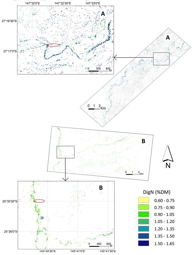
Remote Sens. 2019, 11, 215 3 of 17
We addressed three research questions: 1) is the WV3 data able to accurately estimate and map foliar
DigN; 2) does the WV3 sensor provide better spectral indices to estimate foliar DigN when including
SWIR bands; 3) does the mapped DigN associate with koala tree use?
2. Materials and Methods
2.1. Study Area
The study area was in the Mulgalands bioregion of semi-arid southwest Queensland, Australia.
In summer, average temperature ranges are from 19–35 ◦ C and in winter from 3–19 ◦ C. Average annual
rainfall is about 550 mm in the northeast and decreases to 292 mm in the southwest. Annual rainfall is
highly variable and summer dominant. The major land use is cattle grazing.
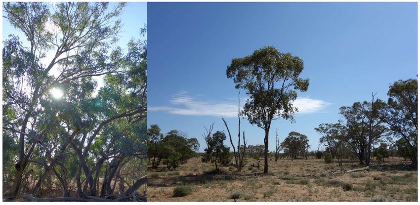
Two landscapes (Landscape A and Landscape B) located ~200 km apart were studied
(Figure 1). The main landforms are riparian strips dominated by Eucalyptus camaldulensis,
Eucalyptus populnea-dominated floodplains and Acacia aneura (mulga) or Acacia harpophylla-dominated
plains (Figure 2). The riparian areas and floodplains in Landscape B also have Eucalyptus coolabah and
some Eucalyptus melanophloia. The four eucalypt species provide forage and shelter to koalas, while the
acacia species provide shelter only. The primary food tree species is E. camaldulensis in the study area.
Figure 1. WorldView-3 satellite images in approximate true colour at Landscape A and Landscape
B captured on 21 November 2015. The map of Queensland at the bottom-left corner shows the
Mulgalands bioregion in grey and the locations of two landscapes as black dots.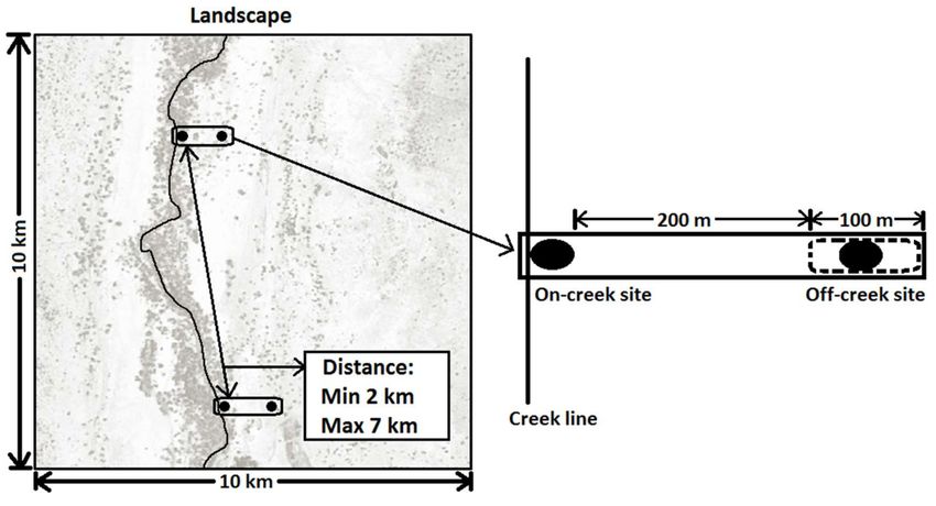
Remote Sens. 2019, 11, 215                                                                                4 of 17

      Figure 2. Field colour photos of Landscape A showing a riparian habitat dominated by
      Eucalyptus camaldulensis (left) and a floodplain habitat dominated by Eucalyptus populnea (right) in
      October 2015.

2.2. Survey Design
     There were two types of data collection: foliage sampling for leaf spectra and leaf DigN
measurement, and acquisition of WV3 data for image spectra and spectral indices calculation.
     In each landscape, two on-creek sites were chosen along creeks (ephemeral watercourse) then
two corresponding off-creek sites were located between 200 m and 300 m from the creek (Figure 3).
On-creek sites and off-creek sites had different tree species and were located in potential koala habitat.
Ten trees from each on-creek site and six trees from each off-creek site were marked for foliage
sampling. Off-creek sites had less trees selected because of its low tree density hence a lower number
of trees available at the site scale (1000s m2 ). From these eight sites, 64 trees were selected in total,
including 35 E. camaldulensis, 7 E. coolabah, 21 E. populnea, and 1 E. melanophloia.

      Figure 3. Survey design of the study showing the position of two on-creek sites (black dots) and two
      off-creek sites (black dots) in a landscape. Corresponding off-creek sites were located between 200 m
      and 300 m from on-creek sites.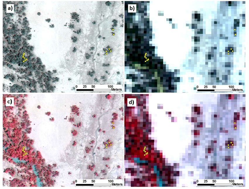
Remote Sens. 2019, 11, 215                                                                         5 of 17

     Ream [29] found that image acquisition in the Mulgalands faced different limitations in wet
and dry seasons. Ground cover (i.e., grass and shrubs) thrives in wet seasons creating mixed pixels
with reflectance from trees and ground vegetation, whereas in dry seasons, senescent ground cover,
bare ground, and sparse tree canopies can create mixed pixels with stronger influence of soil [29].
To minimize the influence of grass, both field sampling and WV3 image acquisition were undertaken in
October and November 2015, the late dry season. Capturing cloud-free satellite images was also more
likely in the dry season. From October 2012 to November 2015, average annual rainfall was 342 mm in
Landscape A and 317 mm in Landscape B. That was much lower than the long-term average annual
rainfall (400–600 mm) and a severe rainfall deficit was reported for this period [31].

2.3. Field Sampling and Leaf Spectral Sampling
      From 19–24 October 2015, the tree species and the location of each selected tree were recorded
using a handheld GPS (Garmin eTrex®30) with a 3 m accuracy on average. To check and correct
the tree GPS location when overlaying on the image, five distinct and widely dispersed locations
(e.g., grid corners, fence corners, and road signs) in each landscape were selected as GPS control points
for image geo-referencing. GPS coordinates and a description of each GPS control point were recorded
by the same GPS device. Leaf samples were collected using a pruning pole from the lower canopy of
all 64 selected trees between 7:00–10:30 a.m.
      Approximately 50 g of leaves were collected from each tree and placed in paper bags to avoid
sunlight for leaf spectral sampling within 30 mins. Fresh leaf spectra were acquired with an ASD
FieldSpec® high-resolution spectrometer between 350 and 2500 nm with 1.1–1.4 nm bandwidth.
A white reference panel was used to standardise and convert relative radiance to reflectance. A leaf
clip and a plant probe with halogen bulb as light source were used to collect leaf surface reflectance.
For each tree, 3 leaves were randomly selected, and 10 spectra were collected from each side. A total
of 60 spectra were collected for each tree and the average spectra were calculated. These averaged
ASD leaf spectra were later resampled to simulate WV3 spectra based on the spectral response of WV3
bands following the methods in Eitel, Long, Gessler, and Smith [17].

2.4. Foliar Chemical Analysis
      After spectral sampling, leaf samples were frozen immediately, and transported frozen to the
University of Queensland where they were freeze-dried and ground (ZM200 Retsch®). Near-infrared
reflectance spectroscopy (NIRS) was used to assist in analysing foliar chemicals. The 64 leaf samples in
this study were collected along with 719 additional leaf samples for a larger koala study carried out in
southwest Queensland. Hence NIRS was done using the 783 leaf samples following Moore, Lawler,
Wallis, Beale, and Foley [9].
      N was quantified using a combustion method with Leco TruMac CN analyser (Leco Corporation,
St. Joseph, MI, USA). DigN was quantified using a two-stage in vitro digestion with pepsin and
cellulose, following the method of DeGabriel, Wallis, Moore, and Foley [14]. DigN concentration was
presented as % dry matter (DM).

2.5. WV3 Image Acquisition and Pre-Processing
    The WV3 multispectral images (DigitalGlobe, USA) used in this study comprised eight
multispectral and eight SWIR bands (Table 1). SWIR bands were collected at 3.7 m spatial resolution
by WV3 but were only made available at 7.5 m due to restrictions imposed by the US Government.
One image was captured for each landscape at 10:40 a.m. AEST, 21 November 2015. Each image
covered an area of 100 km2 and cost AU$109 per km2 . The geo-referencing quality was assessed by
overlaying the satellite images with the field-measured GPS control points in ArcMap (Version 10.4).
Minor deviations were corrected to the nearest 0.31 m (the spatial resolution of WV3 panchromatic
band). Satellite images were atmospherically corrected using Quick Atmospheric Correction in ENVI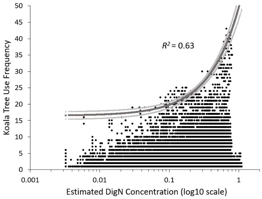
Remote Sens. 2019, 11, 215                                                                                  6 of 17

(Version 5.2). The eight VIS-NIR multispectral bands were resampled to 7.5 m spatial resolution to
calculate indices incorporating both VIS-NIR and SWIR bands.

                Table 1. Details of the sensor bands of WorldView-3 images acquired for this study

                               Band Name            Wavelength (nm)     Spatial Resolution
                              MUL1: Coastal              400–450              1.24 m
                               MUL2: Blue                450–510              1.24 m
                              MUL3: Green                510–580              1.24 m
                              MUL4: Yellow               585–625              1.24 m
                               MUL5: Red                 630–690              1.24 m
                             MUL6: Red Edge              705–745              1.24 m
                               MUL7: NIR1                 770–895             1.24 m
                               MUL8: NIR2                860–1040             1.24 m
                                 SWIR1                  1195–1225             7.5 m
                                 SWIR2                  1550–1590             7.5 m
                                 SWIR3                  1640–1680             7.5 m
                                 SWIR4                  1710–1750             7.5 m
                                 SWIR5                  2145–2185             7.5 m
                                 SWIR6                  2185–2225             7.5 m
                                 SWIR7                  2235–2285             7.5 m
                                 SWIR8                  2295–2365             7.5 m

2.6. Collecting Image Spectra of Sampled Trees
     Image spectra were extracted from the WV3 image pixel corresponding to the GPS position of
each tree (Figure 4). Tree canopies were identified based on GPS position, field photos and the 0.31 m
panchromatic band. In the 1.24 m WV3 images, trees with only epicormic growth were not used if their
canopies were covered by or mixed with neighbouring canopies. For an identified tree canopy, a set of
pixels were selected and the averaged spectra was used. In the 7.5 m WV3 images, most pixels covered
more than one tree hence the trees covered by the same pixel were combined as one averaged tree.

      Figure 4. WorldView-3 image displayed in RGB using bands Blue, Green, Red (a,b) and bands NIR1,
      Red and Blue (c,d) showing the same sample sites in Landscape B at 1.24 m (a,c) and 7.5 m (b,d) spatial
      resolutions. Yellow dots denote tree GPS locations.

     The normalized difference vegetation index (NDVI) was calculated using Red and NIR1 bands
for both field leaf spectra and image spectra [32]. The WV3 NDVI values of some trees were below
0.6, which was lower than the average NDVI of ASD leaf spectra. These trees were not used for this
study as their WV3 spectra were likely to be mixed spectra with other features such as soil, tree trunks,
or big stems rather than pure tree reflection.
     As a result, out of the total 64 trees, 49 trees were used for the 1.24 m WV3 images
(29 E. camaldulensis, 5 E. coolabah, 14 E. populnea, and 1 E. melanophloia) and 27 averaged trees were used
for the 7.5 m WV3 images (19 E. camaldulensis, 2 E. coolabah, 5 E. populnea, and 1 E. melanophloia).
Remote Sens. 2019, 11, 215 7 of 17
2.7. Calculating and Assessing Spectral Indices
Single bands, first derivative spectra and spectral indices were calculated from resampled ASD
spectra, WV3 1.24 m spectra and WV3 7.5 m spectra, to compare the indices’ performance with
leaf-acquired hyperspectral spectra and satellite-derived multispectral data.
These spectral indices were selected from recent studies estimating plant N using remotely-sensed
spectra (Table 2). Normalized difference indices (NDIs) from WorldView-2 (WV2) spectra were
used to estimate grass N concentration [20]. The ratio of transformed chlorophyll absorption in
reflectance index and optimized soil adjusted vegetation index (TCARI/OSAVI) was used to measure
chlorophyll content which is related to nitrogen content [33]. The TCARI/ OSAVI was then modified
by Herrmann, et al. [34] into TCARI1510 /OSAVI1510 because the 1510 nm band is directly related to N
content. Four SWIR-based indices including TCARI1510 /OSAVI1510 from ASD field spectra showed
better estimation for N content of potato fields [34]. Another ratio of modified chlorophyll absorption
ratio index and the second modified triangular vegetation index (MCARI/MTVI2) showed better
performance than TCARI/OSAVI in estimating wheat N content using multispectral data [17].
Table 2. Spectral indices used for estimation of foliar DigN in this study. Spectral bands in the formula
are based on WorldView-3 (WV3) sensor bands. Ra and λa represents the reflectance and the average
wavelength of a certain band. N1.24 is the number of an index from WV3 1.24m spectra. N7.5 is the
number of an index from WV3 7.5m spectra or resampled ASD spectra.
Spectral Index Formula N1.24 N7.5 Reference
Single band Ra 8 16
First derivative Da−b = (Ra − Rb ) / (λa −λb ) 7 15
Normalized difference indices (NDI) NDIa−b = (Ra − Rb ) / (Ra + Rb ) 28 120 [20]
Transformed chlorophyll absorption in reflectance index TCARI = 3[(Red edge − Red) − 0.2(Red edge − Green)
1 1 [33]
(TCARI) (Red edge / Red)]
Optimized soil adjusted vegetation index (OSAVI) OSAVI = 1.16[(NIR1 − Red) / (NIR1 + Red + 0.16)] 1 1 [35]
Transformed chlorophyll absorption in reflectance index TCARI1510 = 3[(Red edge − SWIR2) − 0.2(Red edge -Green)
0 1 Adjusted
1510 (TCARI1510 ) (Red edge / SWIR2)]
from [34]
Optimized soil adjusted vegetation index 1510
OSAVI1510 = 1.16[(NIR1 − SWIR2) / (NIR1 + SWIR2 + 0.16)] 0 1
(OSAVI1510 )
Modified chlorophyll absorption in reflectance index MCARI = [(Red edge − Red) − 0.2(Red edge −
1 1 [36]
(MCARI) Green)] (Red edge / Red)
MTVI2 = [1.8(NIR1 − Green) − 3.75(Red − Green)] / sqrt
Modified triangle vegetation index 2 (MTVI2) 1 1 [37]
[(2NIR1 + 1) ˆ2 − 6NIR1 + 5sqrt(Red) − 0.5]
TCARI / OSAVI 1 1
[17]
Combined index MCARI / MTVI2 1 1
TCARI1510 / OSAVI1510 0 1 [34]
The correlation coefficients between the spectral indices and DigN concentrations were used to
estimate the performance of indices. For the index with the best correlation coefficients, linear and
second-order regression equations were used to determine the best estimation of DigN. The coefficient
of determination (R2 ), p-value and root mean square error (RMSE) were used to compare the
performance of the spectral indices. All data analysis was performed in Excel.
2.8. Mapping DigN with Selected Index
Because the average NDVI of ASD leaf spectra was 0.6, a mask of NDVI > 0.6 was applied to the
WV3 images to subset the areas of vegetation. Using the region of interest (ROI) tool in ENVI, a plot
of average spectra of eucalypt trees, non-eucalypt trees (A. aneura and Geijera parviflora mixed) and
dense grass patches (mixed species) was created to find ways to mask out grass and non-eucalypt
trees. The accuracy of the vegetation masks was visually assessed in ArcMap. A set of 100 random
pixels were created within the final masked image. Then they were checked visually using the 0.31 m
panchromatic image and the 1.24 m VNIR image to confirm whether they cover trees. The equation of
the selected index for DigN was applied to the masked image in ENVI. The foliar DigN concentrations
of eucalypt tree areas were mapped and displayed in colour.Remote Sens. 2019, 11, 215 8 of 17
2.9. Application of DigN Mapping Method to WV2 Image
The WV2 image was collected at 10:58AM AEST, 16 October 2012, which was a similar time
and season as the WV3 images. It covered a landscape (270 km2 at 2 m spatial resolution) adjacent
to the south of Landscape A which has the same landform and vegetation. The WV2 image was
atmospherically corrected using Quick Atmospheric Correction in ENVI (Version 5.2). The mapping
method described above was applied to this image. Vegetation masks were applied to the image to
subset areas of trees. The accuracy of the vegetation masks was visually assessed in ArcMap. A set
of 100 random pixels were created within the final masked image. Then they were checked visually
using the 0.46 m panchromatic image and the 2 m VNIR image to confirm whether they cover trees.
The equation of the selected index for DigN was applied to the masked image using band math in
ENVI to produce a map of foliar DigN concentrations.
2.10. Associating Mapped DigN from WV2 Image with Koala Tree Use Data
Koala tracking and data collection was described by Davies, Gramotnev, Seabrook, Bradley,
Baxter, Rhodes, Lunney, and McAlpine [28]. The locations of five koalas in this landscape were
recorded as GPS points from August 2010 to November 2011. All GPS points were overlaid in ArcMap.
Because there were no field-measured GPS control points, we reduced potential errors by observing
and checking the GPS points against koalas’ habits (i.e., spend more time in trees than on the ground,
do not swim). If a group of neighbouring points were on ground/water surface and have a tree to
the same distance and direction nearby on the WV2 image, they were manually spatially adjusted
to tree canopies Only nocturnal locations (5:00 p.m. to 06:00 a.m.) were used because koalas mainly
feed during this time and their tree use during the night was more likely to be influenced by foliar
DigN [38]. These points were then converted to a raster layer (sum of koala tree use) with the same
pixel size as the DigN map which corresponds with the WV2 image (2 m spatial resolution). As the
accuracy of most GPS units was within a 5 m radius, an averaging convolution filter for a 11 × 11
pixels moving window was applied to the layer in ENVI to calculate the density of koala tree use.
The same convolution process was applied to the DigN map. DigN and density of koala tree use data
were queried and extracted in TerrSet (Version 18.3), then analysed using quantile regression in XLStat
(www.xlstat.com) at different quantiles (0.200–0.999). Quantile regression can estimate potential causal
relationships between variables at certain quantiles when not all predictive factors are measured for
variable ecological responses [39]. Hence quantile regression is suitable to this case because koala tree
use can be affected by DigN and other factors, such as plant secondary metabolites and tree size [8].
3. Results
3.1. Laboratory Measures of Foliar Chemistry
Table 3 summarises the measured DigN and N concentrations for all samples (n = 64), samples for
1.24 m WV3 images (n = 49) and 7.5 m WV3 images (n = 27). The Pearson correlation coefficient
between DigN and N concentration was r = 0.46 (P < 0.001).
Table 3. DigN and N concentrations (% dry matter) of all samples, sample subsets for WorldView-3
images at 1.24 m and 7.5 m spatial resolutions
Response Variable Samples Size Mean Min Max SD CV (%)
N 64 1.65 1.09 2.20 0.22 13.12
N 1.24 m 49 1.65 1.09 2.20 0.22 13.62
N 7.5 m 27 1.66 1.20 2.20 0.23 13.56
DigN 64 1.12 0.35 1.86 0.33 29.12
DigN 1.24 m 49 1.14 0.35 1.86 0.34 29.86
DigN 7.5 m 27 1.20 0.35 1.86 0.35 29.46Remote Sens. 2019, 11, 215 9 of 17
3.2. Estimation of DigN Concentration from Resampled ASD Spectra and WV3 Spectra
The best index to estimate foliar DigN concentration was NDICoastal-NIR1 using WV3 7.5 m spectra.
Its regression relationship with DigN concentration (R2 = 0.70, P < 0.001, RMSE = 0.191% DM) is shown
in Figure 5.
Figure 5. Regression of the relationship between digestible nitrogen (DigN; % dry matter) and NDI
of MUL1 (Coastal) and MUL7 (NIR1) bands. NDIs were calculated from WorldView-3 images of
Landscape A and B at 7.5 m spatial resolution.
The performance of indices of DigN concentration in WV3 spectra was different from that in
resampled ASD spectra (Table 4). The first derivative including SWIR bands (DSWIR6-7 and DSWIR7-8 )
were better than DRed edge-NIR1 in resampled ASD spectra but this was reversed in WV3 spectra.
Similarly, single band SWIR3 performed well with resampled ASD spectra while coastal was better
with WV3 7.5 m spectra. The NDIs were poor at estimating DigN from resampled ASD spectra but
performed well with WV3 7.5 m data. The NDIs using only VNIR bands performed better than those
containing the SWIR band in WV3 7.5 m spectra.Remote Sens. 2019, 11, 215 10 of 17
Table 4. Coefficient of determination (R2 ), p-value and RMSE (% dry matter) for various spectral
indices used as regression estimators of foliar digestible nitrogen concentration (DigN; % dry matter)
in eucalypts. Spectral indices were calculated from three datasets including resampled ASD spectra,
WorldView-3 (WV3) 1.24 m spectra and WV3 7.5 m spectra. R2 over 0.40 are shown in bold text.
Resampled ASD WV3 1.24 m WV3 7.5 m
Spectral Index
R2 p RMSE R2 p RMSE R2 p RMSE
MCARI 0.00 0.674 0.324 0.03 0.242 0.332 0.18 0.026 0.312
MTVI2 0.02 0.254 0.324 0.13 0.011 0.315 0.42Remote Sens. 2019, 11, 215 11 of 17
In both landscapes, the foliar DigN along creek lines stood out on the maps where the tree density was
relatively higher (Figure 7). Overall foliar DigN concentration was lower in Landscape B. The trees on
the floodplain (around 300 m away from the creek) in Landscape A showed high DigN concentrations
but the species of these tree were uncertain because of a lack of field reference observation. GPS collar
data showed koalas in the Mulgalands spent more than 80% of their time on average within riverine
habitat [28] and koalas tend to be found within 300 m of creek lines [40]. Therefore, the trees 300 m
away from creek were of less importance in this study and were not observed in the field. The cluster
of higher DigN in the zoomed-in area of Landscape B was a house garden with frequent irrigation,
which contained mature E. camaldulensis (grown from local seedlings), non-eucalypt trees, bushes,
and grass.
Figure 7. Maps of foliar digestible nitrogen (DigN) at Landscape A and B in colour. Black boxes in full
maps indicate locations of zoomed-in areas. Red circles in zoomed-in areas indicate locations of sample
sites. Features in non-tree areas (soil, water and grass) are white.Remote Sens. 2019, 11, 215 12 of 17
3.4. Relationship between Mapped DigN from WV2 Image with Koala Tree Use
There were 1,428 GPS records of the occurrence of koalas at night time. After averaging
convolution, there were 66,926 tree pixels (2 m) with the frequency of koala tree use which was
between 1 to 43 (mean = 2.58).
For DigN mapping, a mask of NDVI>0.57 was applied to the WV2 images to subset the areas
of vegetation. Based on average spectra of grass and different tree species (Figure S1), vegetation
areas with RNIR1 > 0.59 were masked out to exclude grass, whereas the remaining tree areas with
(RNIR1 –RRed ) < 0.28 were masked out to exclude the known non-eucalypt trees. All 100 random pixels
from the masked image in Landscape C were visually confirmed that they cover trees. Foliar DigN
concentration of each pixel (2 m) was estimated using the WV2 spectra and the NDICoastal-NIR1 spectral
index. The estimated DigN concentration of these 66,926 tree pixels was between 0 to 1.11% DM
(mean = 0.21% DM).
Quantile regression showed improvement in fit being at higher quantile (Figure S2). The highest
coefficients of determination between the frequency of koala tree use and the estimated DigN
concentration from WV2 spectra was in the 0.999 quantile (Figure 8, R2 = 0.63, P < 0.001).
Figure 8. Correlation between koala tree use frequency (as mapped in the field in 2010 and 2011) and
log10 transformed estimated DigN concentration (% dry matter) from the WV2 image of 2012 with
quantile regression fitted line for the 0.999 quantile (dark grey) and 95% confidence bounds (light grey).
4. Discussion
This study assessed the potential of using WV3 multispectral data to map foliar DigN
concentrations of eucalypt trees from two landscapes in the semi-arid Mulgalands bioregion, Australia.
The spectral index NDICoastal-NIR1 was found to satisfactorily estimate foliar DigN concentrations.
The DigN mapping method using this index were tested by linking previous koala tree use frequency
with mapped DigN from a WV2 image of an independent landscape in the study area. Results indicatedRemote Sens. 2019, 11, 215 13 of 17
greater koala tree use for trees with higher estimated DigN, which is consistent with previous
studies [8,41]. Therefore, it is possible to estimate and map the variation in eucalypt foliar DigN
over large areas using WV3- or WV2-derived multispectral data and these estimates are meaningful
for the evaluation of koala habitat suitability.
4.1. Spectral Indices to Estimate and Map Foliar DigN
This is the first attempt we know of to estimate foliar DigN using satellite-derived spectra.
Previously, Youngentob, Renzullo, Held, Jia, Lindenmayer, and Foley [19] successfully estimated
foliar DigN using airborne hyperspectral spectra. DigN is an integrated foliar nutritional
measurement influenced by concentrations of nitrogen, tannins, cellulose, and lignin [14].
Consequently, the relationship between spectral indices and foliar DigN concentration would be
indirect. The best index from WV3 spectra, NDICoastal-Blue , showed good estimation capability.
Regarding the first and second research questions (whether WV3 can be used for DigN mapping and
whether SWIR bands can improve the mapping), this study suggested that the WV3 sensor can provide
spectral indices to estimate and map foliar DigN in eucalypt across a landscape but the best index does
not include SWIR bands.
It was interesting that the ASD and WV3 spectra both returned useful, but different spectral
indices, from distinct regions of the spectrum. In the resampled ASD spectra, the best-performing
spectral indices (R2 > 0.4) were obtained from the SWIR region but the best spectral indices from
WV3 spectra were from the VNIR region (Coastal, Blue, NIR1, and NIR2) instead. Because the
best-performing spectral indices from ASD and WV3 spectra used bands of absorption features of
DigN associated chemicals, we suggest that such differences may be related to issues of (1) sampling
scale, with the leaf scale of ASD spectra versus the canopy scale of WV3 spectra, (2) atmospheric
effects which apply to WV3 spectra but not to ASD spectra, and 3) the potential signal integrity
and signal to noise ratio differences between the two different sensors [42]. In the SWIR region,
SWIR3, 6, and 8 contain nitrogen absorption features at 1645, 2180, 2240, 2300, and 2350 nm [19,43].
SWIR3 also contains tannin and lignin absorption features (1658, 1675, and 1668 nm), whereas SWIR7
has absorption features of cellulose (2280 nm) and lignin (2272 nm) which influence dry matter
digestibility [43,44]. In the VNIR region, apart from the absorption features of chlorophyll at 430 and
460 nm or nitrogen at 808, 868, 910, and 1020 nm [43,45,46], spectral indices using the four VNIR bands
also contain absorption features of tannins (803 nm in NIR1, 948 and 993 nm in NIR2) and lignin
(478 nm in Blue) [47,48].
4.2. Better Performance of WV3 7.5 m Spectra than 1.24 m Spectra
When estimating foliar DigN, most spectral indices performed better (higher R2 , lower RMSE)
with WV3 7.5 m spectra than with WV3 1.24 m spectra. This may be caused by the difficulty of
identifying pure pixels for a single tree canopy from WV3 1.24 m images. The canopies of dense
E. camaldulensis along creeks overlap and one pixel may contain the leaf reflection of more than one
tree. Therefore, defining the tree spectra of one tree from WV3 1.24 m images based on tree trunk GPS
risks including the reflection of its neighbours. In addition, the accuracy of the handheld GPS is about
3 m which is less than the spatial resolution of WV3 1.24 m spectra. The pixel selected based on a GPS
coordinate may not precisely represent the pure spectra of a specific tree, giving a lower correlation
with foliar DigN. In contrast, at 7.5 m spatial resolution, when one pixel covered more than one tree
GPS, its spectra were defined as the combined tree spectra of the trees within this pixel. The combined
tree spectra were correlated with the combined foliar DigN of these trees.
This does not mean WV3 1.24 m data is less useful. Tree sampling in this study was designed
primarily to select koala food trees for foliar chemical analysis, rather than to be compared with satellite
imagery. A better sampling design for a similar remote sensing study would have sampled more trees
and chosen isolated trees with denser and bigger canopies that were identifiable in the image [19] and
used higher-accuracy differential GPS location data. These measures may improve spectral indicesRemote Sens. 2019, 11, 215 14 of 17
performance in WV3 1.24 m data. This requirement for isolated trees constrains the development
and validation of spectral indices, but need not constrain subsequent estimation of habitat suitability,
where pixels capturing more than one tree return an estimate of mean nutritional quality which is
nonetheless useful for habitat mapping purposes.
4.3. Mapped DigN to Evaluate Koala Habitat Suitability
Our results show that trees with higher foliar DigN concentration can have any level of koala
use, but low DigN trees only have low koala use. Although koalas spend more time feeding in trees
with higher DigN concentrations, koala tree use is also influenced by other factors such as foliar
plant secondary metabolites, tree species, and tree size [8]. Low koala densities in the study region
also mean that many suitable trees may never be encountered by koalas. That is why the estimated
DigN concentration only explained part of the variation of koala tree use frequency. For example,
some trees with very high estimated foliar DigN concentration but very low koala tree use frequency
were located on the flood plain where koalas spent less than 20% of time during the tracking period [28].
Although there were unmeasured factors, the mapped DigN concentration from WV2 proved to be
a limiting factor for koala tree use frequency. In responding to the third research question, the mapped
DigN is associated with koala tree use and this DigN mapping method is useful in assessing koala
habitat suitability.
In addition, testing the relationship between mapped DigN and koala tree used worked as
a validation of the DigN mapping method. The validation is independent for using an image of
a different sensor, landscape and time, however it is indirect by using koala tree use instead of field
measured foliar DigN. Therefore, we were not able to measure the accuracy of applying the DigN
mapping method on WV2.
5. Conclusions
We have reported the first attempt to correlate satellite-derived multispectral data with foliar
DigN, which is an important measure of food quality for koalas. The foliar chemical variations of
koala food tree species indicate food availability and quality more precisely than the presence or
absence of food tree species [8]. Hence, the DigN mapping method can improve the mapping of
high quality habitat at the landscape scale for effective koala conservation and habitat management.
Because this DigN mapping method was developed across two landscapes and four eucalypt species,
then tested for a new landscape with similar eucalypt species, we concluded that it can be applied to
new open eucalypt woodlands with similar tree species which are, for example, widely distributed in
the Murray–Darling basin in Australia. This technique, once tested to assess its reliability with different
tree species, could be used to validate the accuracy of coarse koala habitat mapping based on vegetation
communities and improve koala habitat classification by adding finer foliar nutritional information.
Supplementary Materials: The following are available online at http://www.mdpi.com/2072-4292/11/2/215/s1,
Figure S1: Average reflectance of eucalypt tree (solid line), non-eucalypt tree and grass (dashed lines) at eight
spectral bands from the WorldView-2 image at 2 m spatial resolution, Figure S2: Coefficients of determination for
quantile regression for 30 values of quantiles (from 0.970 to 0.999), where y is the frequency of koala tree use and
x is estimated DigN concentration from WorldView-2 spectra.
Author Contributions: Conceptualization, H.W., N.L., L.S., and C.M.; Methodology, H.W. and N.L.;
Validation, H.W. and N.L.; Formal analysis, H.W. and N.L.; Investigation, H.W., N.L., and B.M.; Resources,
L.S. and B.M.; Writing—original draft preparation, H.W.; Writing—review and editing, N.L., L.S., B.M., and C.M.;
Visualization, H.W.; Supervision, C.M.; Project Administration, H.W.; Funding Acquisition, H.W., N.L., and C.M.
Funding: This research was funded by Australia Research Council Future Fellowship (FT100100338),
Endeavour Scholarship (Prime Minister’s Australia Asia Scholarship, 3704_2014) and Wildlife Preservation
Society of Queensland (Wildlife Queensland student research grant 2016).
Acknowledgments: Many thanks to landholders for the permission of fieldwork and sharing knowledge of their
lands, to all field volunteers for their assistance, and to Dr. Glen Fox for the access to WinISI.
Conflicts of Interest: The authors declare no conflict of interest.Remote Sens. 2019, 11, 215 15 of 17
References
1. Environment Protection Authority. Koala Habitat Mapping Pilot: NSW State Forests. Available online:
www.epa.nsw.gov.au (accessed on 10 December 2016).
2. Callaghan, J.; McAlpine, C.; Thompson, J.; Mitchell, D.; Bowen, M.; Rhodes, J.; de Jong, C.; Sternberg, R.; Scott, A.
Ranking and mapping koala habitat quality for conservation planning on the basis of indirect evidence of tree-species
use: A case study of Noosa Shire, south-eastern Queensland. Wildl. Res. 2011, 38, 89–102. [CrossRef]
3. GHD. South East Queensland Koala Habitat Assessment and Mapping Project. Available online:
https://data.qld.gov.au/dataset/koala-planning-areas-version-1-2-south-east-queensland-data-package
(accessed on 21 April 2018).
4. Lunney, D.; Phillips, S.; Callaghan, J.; Coburn, D. Determining the distribution of koala habitat across a shire as
a basis for conservation: A case study from Port Stephens, New South Wales. Pac. Conserv. Biol. 1998, 4, 186–196.
[CrossRef]
5. McAlpine, C.; Rhodes, J.; Callaghan, J.; Bowen, M.; Lunney, D.; Mitchell, D.; Pullar, D.; Possingham, H.
The importance of forest area and configuration relative to local habitat factors for conserving forest
mammals: A case study of koalas in Queensland, Australia. Biol. Conserv. 2006, 132, 153–165. [CrossRef]
6. Moore, B.; Wallis, I.; Marsh, K.; Foley, W. The role of nutrition in the conservation of the marsupial folivores
of eucalypt forests. In Conservation of Australia’s Forest Fauna; Lunney, D., Ed.; Royal Zoological Society of
New South Wales: Mosman, Australia, 2004; pp. 549–575.
7. Woinarski, J.; Burbidge, A. Phascolarctos Cinereus. Available online: https://www.iucnredlist.org/species/
16892/21960344 (accessed on 5 June 2017).
8. Marsh, K.; Moore, B.; Wallis, I.; Foley, W. Feeding rates of a mammalian browser confirm the predictions of
a ‘foodscape’ model of its habitat. Oecologia 2014, 174, 873–882. [CrossRef] [PubMed]
9. Moore, B.; Lawler, I.; Wallis, I.; Beale, C.; Foley, W. Palatability mapping: A koala’s eye view of spatial
variation in habitat quality. Ecology 2010, 91, 3165–3176. [CrossRef] [PubMed]
10. Munks, S.A.; Corkrey, R.; Foley, W.J. Characteristics of arboreal marsupial habitat in the semi-arid woodlands
of northern Queensland. Wildl. Res. 1996, 23, 185–195. [CrossRef]
11. Wu, H.; McAlpine, C.A.; Seabrook, L.M. The dietary preferences of koalas, Phascolarctos cinereus, in southwest
Queensland. Aust. Zool. 2012, 36, 93–102. [CrossRef]
12. Mertl-Millhollen, A.S.; Rambeloarivony, H.; Miles, W.; Kaiser, V.; Gray, L.; Dorn, L.; Williams, G.;
Rasamimanana, H. The influence of tamarind tree quality and quantity on Lemur catta behavior.
In Ringtailed Lemur Biology; Springer: New York, NY, USA, 2006; pp. 102–118.
13. Simmen, B.; Tamaud, L.; Hladik, A. Leaf nutritional quality as a predictor of primate biomass: Further evidence of
an ecological anomaly within prosimian communities in Madagascar. J. Trop. Ecol. 2012, 28, 141–151. [CrossRef]
14. DeGabriel, J.; Wallis, I.; Moore, B.; Foley, W. A simple, integrative assay to quantify nutritional quality of
browses for herbivores. Oecologia 2008, 156, 107–116. [CrossRef]
15. DeGabriel, J.L.; Moore, B.D.; Foley, W.J.; Johnson, C.N. The effects of plant defensive chemistry on nutrient
availability predict reproductive success in a mammal. Ecology 2009, 90, 711–719. [CrossRef] [PubMed]
16. Skidmore, A.K.; Ferwerda, J.G.; Mutanga, O.; Van Wieren, S.E.; Peel, M.; Grant, R.C.; Prins, H.H.T.; Balcik, F.B.;
Venus, V. Forage quality of savannas—Simultaneously mapping foliar protein and polyphenols for trees and
grass using hyperspectral imagery. Remote Sens. Environ. 2010, 114, 64–72. [CrossRef]
17. Eitel, J.; Long, D.; Gessler, P.; Smith, A. Using in-situ measurements to evaluate the new RapidEye™ satellite
series for prediction of wheat nitrogen status. Int. J. Remote Sens. 2007, 28, 4183–4190. [CrossRef]
18. Govender, M.; Chetty, K.; Naiken, V.; Bulcock, H. A comparison of satellite hyperspectral and multispectral
remote sensing imagery for improved classification and mapping of vegetation. Water 2008, 34, 147–154.
19. Youngentob, K.; Renzullo, L.; Held, A.; Jia, X.; Lindenmayer, D.; Foley, W. Using imaging spectroscopy to
estimate integrated measures of foliage nutritional quality. Methods Ecol. Evol. 2012, 3, 416–426. [CrossRef]
20. Adjorlolo, C.; Mutanga, O.; Cho, M.A. Estimation of canopy nitrogen concentration across C3 and C4 grasslands
using Worldview-2 multispectral data. IEEE J. Sel. Top. Appl. Earth Obs. Remote Sens. 2014, 7, 4385–4392. [CrossRef]
21. Zengeya, F.; Mutanga, O.; Murwira, A. Linking remotely sensed forage quality estimates from WorldView-2
multispectral data with cattle distribution in a savanna landscape. Int. J. Appl. Earth Obs. Geoinf. 2013, 21, 513–524.
[CrossRef]Remote Sens. 2019, 11, 215 16 of 17
22. Bagheri, N.; Ahmadi, H.; Alavipanah, S.K.; Omid, M. Multispectral remote sensing for site-specific nitrogen
fertilizer management. Pesqui. Agropecu. Bras. 2013, 48, 1394–1401. [CrossRef]
23. Boegh, E.; Houborg, R.; Bienkowski, J.; Braban, C.F.; Dalgaard, T.; Van Dijk, N.; Dragosits, U.; Holmes, E.;
Magliulo, V.; Schelde, K.; et al. Remote sensing of LAI, chlorophyll and leaf nitrogen pools of crop- and
grasslands in five European landscapes. Biogeosciences 2013, 10, 6279–6307. [CrossRef]
24. Reyniers, M.; Vrindts, E. Measuring wheat nitrogen status from space and ground-based platform. Int. J.
Remote Sens. 2006, 27, 549–567. [CrossRef]
25. Zandler, H.; Brenning, A.; Samimi, C. Potential of space-borne hyperspectral data for biomass quantification
in an arid environment: Advantages and limitations. Remote Sens. 2015, 7, 4565–4580. [CrossRef]
26. Chemura, A.; Mutanga, O.; Odindi, J.; Kutywayo, D. Mapping spatial variability of foliar nitrogen in coffee
(Coffea arabica L.) plantations with multispectral Sentinel-2 MSI data. ISPRS J. Photogramm. Remote Sens. 2018, 138.
[CrossRef]
27. Verma, N.; Lamb, D.; Reid, N.; Wilson, B. Comparison of canopy volume measurements of scattered eucalypt
farm trees derived from high spatial resolution imagery and LiDAR. Remote Sens. 2016, 8, 388. [CrossRef]
28. Davies, N.; Gramotnev, G.; Seabrook, L.; Bradley, A.; Baxter, G.; Rhodes, J.; Lunney, D.; McAlpine, C.
Movement patterns of an arboreal marsupial at the edge of its range: A case study of the koala. Mov. Ecol.
2013, 1, 8. [CrossRef] [PubMed]
29. Ream, B. Mapping Eucalypts in South-West Queensland: Answering the Question Can Fine Resolution
Satellite Remote Sensing Be Used to Map Eucalypt Composition. Ph.D. Thesis, The University of Queensland,
Brisbane, Australia, 2013.
30. Seabrook, L.; McAlpine, C.; Rhodes, J.; Baxter, G.; Bradley, A.; Lunney, D. Determining range edges:
Habitat quality, climate or climate extremes? Divers. Distrib. 2014, 20, 95–106. [CrossRef]
31. Australian Government Bureau of Meteorology Climate Data Online. Available online:
http://www.bom.gov.au/water/landscape/ (accessed on 31 October 2016).
32. Rouse, J.; Harlan, J.; Haas, R.; Schell, J.; Deering, D. Monitoring the Vernal Advancement and
Retrogradation (Green Wave Effect) of Natural Vegetation; Remote Sensing Center, Texas A&M University:
Colleg Station, TX, USA, 1974.
33. Haboudane, D.; Miller, J.; Tremblay, N.; Zarco-Tejada, P.; Dextraze, L. Integrated narrow-band vegetation
indices for prediction of crop chlorophyll content for application to precision agriculture. Remote Sens. Environ.
2002, 81, 416–426. [CrossRef]
34. Herrmann, I.; Karnieli, A.; Bonfil, D.; Cohen, Y.; Alchanatis, V. SWIR-based spectral indices for assessing
nitrogen content in potato fields. Int. J. Remote Sens. 2010, 31, 5127–5143. [CrossRef]
35. Rondeaux, G.; Steven, M.; Baret, F. Optimization of soil-adjusted vegetation indices. Remote Sens. Environ.
1996, 55, 95–107. [CrossRef]
36. Daughtry, C.; Walthall, C.; Kim, M.; de Colstoun, E.B.; McMurtrey, J. Estimating corn leaf chlorophyll
concentration from leaf and canopy reflectance. Remote Sens. Environ. 2000, 74, 229–239. [CrossRef]
37. Haboudane, D.; Miller, J.; Pattey, E.; Zarco-Tejada, P.; Strachan, I. Hyperspectral vegetation indices and novel
algorithms for predicting green LAI of crop canopies: Modeling and validation in the context of precision
agriculture. Remote Sens. Environ. 2004, 90, 337–352. [CrossRef]
38. Marsh, K.J.; Moore, B.D.; Wallis, I.R.; Foley, W.J. Continuous monitoring of feeding by koalas highlights
diurnal differences in tree preferences. Wildl. Res. 2014, 40, 639–646. [CrossRef]
39. Cade, B.; Noon, B. A gentle introduction to quantile regression for ecologists. Front. Ecol. Environ. 2003, 1, 412–420.
[CrossRef]
40. Davies, N.; (The University of Queensland, Brisbane, Australia). Personal communication, 2014.
41. Stalenberg, E.; Wallis, I.; Cunningham, R.; Allen, C.; Foley, W. Nutritional correlates of koala persistence in
a low-density population. PLoS ONE 2014, 9, e113930. [CrossRef] [PubMed]
42. Mutanga, O.; Adam, E.; Adjorlolo, C.; Abdel-Rahman, E.M. Evaluating the robustness of models developed
from field spectral data in predicting African grass foliar nitrogen concentration using WorldView-2 image
as an independent test dataset. Int. J. Appl. Earth Obs. Geoinf. 2015, 34, 178–187. [CrossRef]
43. Curran, P.J. Remote sensing of foliar chemistry. Remote Sens. Environ. 1989, 30, 271–278. [CrossRef]
44. Soukupova, J.; Rock, B.N.; Albrechtova, J. Spectral characteristics of lignin and soluble phenolics in the near
infrared- a comparative study. Int. J. Remote Sens. 2002, 23, 3039–3055. [CrossRef]Remote Sens. 2019, 11, 215 17 of 17
45. Coops, N.; Smith, M.; Martin, M.; Ollinger, S. Prediction of eucalypt foliage nitrogen content from
satellite-derived hyperspectral data. IEEE Trans. Geosci. Remote Sens. 2003, 41, 1338–1346. [CrossRef]
46. William, P.C. Implementation of Near-infrared technology. In Near-Infrared Technology: In the Agricultural
and Food Industries, 2nd ed.; Williams, P.C., Norris, K., Eds.; American Association of Cereal Chemists:
St. Paul, MN, USA, 2001; pp. 145–169.
47. Curran, P.; Dungan, J.; Peterson, D. Estimating the foliar biochemical concentration of leaves with reflectance
spectrometry. Remote Sens. Environ. 2001, 76, 349–359. [CrossRef]
48. Ferwerda, J.; Skidmore, A.; Stein, A. A bootstrap procedure to select hyperspectral wavebands related to
tannin content. Int. J. Remote Sens. 2006, 27, 1413–1424. [CrossRef]
© 2019 by the authors. Licensee MDPI, Basel, Switzerland. This article is an open access
article distributed under the terms and conditions of the Creative Commons Attribution
(CC BY) license (http://creativecommons.org/licenses/by/4.0/).You can also read