COMPARING THE SPATIAL ACCURACY OF DIGITAL SURFACE MODELS FROM FOUR UNOCCUPIED AERIAL SYSTEMS: PHOTOGRAMMETRY VERSUS LIDAR - MDPI
←
→
Page content transcription
If your browser does not render page correctly, please read the page content below
remote sensing
Article
Comparing the Spatial Accuracy of Digital Surface
Models from Four Unoccupied Aerial Systems:
Photogrammetry Versus LiDAR
Stephanie R. Rogers 1, * , Ian Manning 2 and William Livingstone 2
 1    Department of Geosciences, Auburn University, Auburn, AL 36849, USA
 2    Applied Research, Nova Scotia Community College, Lawrencetown, NS B0S 1M0, Canada;
      ian.manning@nscc.ca (I.M.); william.livingstone@nscc.ca (W.L.)
 *    Correspondence: s.rogers@auburn.edu; Tel.: +1-334-844-4069

 Received: 30 July 2020; Accepted: 27 August 2020; Published: 29 August 2020

 Abstract: The technological growth and accessibility of Unoccupied Aerial Systems (UAS) have
 revolutionized the way geographic data are collected. Digital Surface Models (DSMs) are an integral
 component of geospatial analyses and are now easily produced at a high resolution from UAS images
 and photogrammetric software. Systematic testing is required to understand the strengths and
 weaknesses of DSMs produced from various UAS. Thus, in this study, we used photogrammetry to
 create DSMs using four UAS (DJI Inspire 1, DJI Phantom 4 Pro, DJI Mavic Pro, and DJI Matrice 210)
 to test the overall accuracy of DSM outputs across a mixed land cover study area. The accuracy and
 spatial variability of these DSMs were determined by comparing them to (1) 12 high-precision GPS
 targets (checkpoints) in the field, and (2) a DSM created from Light Detection and Ranging (LiDAR)
 (Velodyne VLP-16 Puck Lite) on a fifth UAS, a DJI Matrice 600 Pro. Data were collected on July 20,
 2018 over a site with mixed land cover near Middleton, NS, Canada. The study site comprised an
 area of eight hectares (~20 acres) with land cover types including forest, vines, dirt road, bare soil,
 long grass, and mowed grass. The LiDAR point cloud was used to create a 0.10 m DSM which
 had an overall Root Mean Square Error (RMSE) accuracy of ±0.04 m compared to 12 checkpoints
 spread throughout the study area. UAS were flown three times each and DSMs were created with the
 use of Ground Control Points (GCPs), also at 0.10 m resolution. The overall RMSE values of UAS
 DSMs ranged from ±0.03 to ±0.06 m compared to 12 checkpoints. Next, DSMs of Difference (DoDs)
 compared UAS DSMs to the LiDAR DSM, with results ranging from ±1.97 m to ±2.09 m overall.
 Upon further investigation over respective land covers, high discrepancies occurred over vegetated
 terrain and in areas outside the extent of GCPs. This indicated LiDAR’s superiority in mapping
 complex vegetation surfaces and stressed the importance of a complete GCP network spanning the
 entirety of the study area. While UAS DSMs and LiDAR DSM were of comparable high quality when
 evaluated based on checkpoints, further examination of the DoDs exposed critical discrepancies
 across the study site, namely in vegetated areas. Each of the four test UAS performed consistently
 well, with P4P as the clear front runner in overall ranking.

 Keywords: UAS; LiDAR; digital surface models; DSM; geographic data collection

1. Introduction
     Digital Elevation Models (DEMs) are geometric representations of the topography where elevations
are represented as pixels in raster format [1]. DEMs are categorized into Digital Terrain Models (DTMs),
which represent topography void of surface features; and Digital Surface Models (DSMs), which depict
the top surfaces of features elevated above the earth, including buildings, trees, and towers (Figure 1).

Remote Sens. 2020, 12, 2806; doi:10.3390/rs12172806                      www.mdpi.com/journal/remotesensing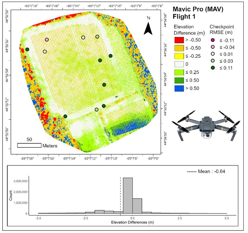
Remote Sens. 2020, 12, 2806 2 of 17
Historically, DEMs were arduously produced from surveyed field data, contour lines on topographic
maps, and photogrammetry from aerial photography [2,3]. DEM accuracy and production efficiency
greatly improved with the onset of Light Detection and Ranging (LiDAR). LiDAR data are costly to
obtain for small areas, as they are collected from piloted aircraft (airborne LiDAR) and/or from ground
Remote Sens. 2020, 12, x FOR PEER REVIEW 2 of 18
level (terrestrial LiDAR). Airborne LiDAR is more efficient for regional scale studies, while terrestrial
contour lines
LiDAR is optimal on topographic
for hyperlocal maps, [4].
scales and photogrammetry
Additionally, from bothaerial photography
require extensive [2,3].expertise
DEM in data
accuracy and production efficiency greatly improved with the onset of Light Detection and Ranging
acquisition and processing. Although LiDAR has produced some of the most accurate
(LiDAR). LiDAR data are costly to obtain for small areas, as they are collected from piloted aircraft
representations
of the Earth’s surface,
(airborne LiDAR)its and/or
availability
from groundandlevel
accessibility are technically,
(terrestrial LiDAR). Airborne LiDARor financially, challenging
is more efficient for for
regional
sections of the userscale studies,
group. while terrestrial
However, LiDAR push
the recent is optimal for hyperlocal
towards makingscales [4]. Additionally,
state-funded both data more
LiDAR
require extensive expertise in data acquisition and processing. Although LiDAR has produced some
readily available through online portals [5–7] will improve availability. Additionally, the technological
of the most accurate representations of the Earth’s surface, its availability and accessibility are
growth andtechnically,
accessibility of Unoccupied
or financially, challengingAerial Systems
for sections of the(UAS) have
user group. revolutionized
However, the production
the recent push
of geographic information
towards [8,9], furthering
making state-funded LiDAR data collection
more readilyavailability of high-resolution
available through online portals [5–7]imagery
will that can
improve availability. Additionally, the technological growth and accessibility of Unoccupied Aerial
be processed to create orthophotomosaics and DEMs. DEMs are input layers in many Geographic
Systems (UAS) have revolutionized the production of geographic information [8,9], furthering
Informationcollection
System availability
(GIS) calculations and applications.
of high-resolution imagery that canDSMs, specifically,
be processed are a critical component of
to create orthophotomosaics
geospatial analyses,
and DEMs.ranging
DEMs arefrom inputprecision agriculture
layers in many Geographic [10] to urban
Information development
System [11,12],
(GIS) calculations andforestry [13],
applications.
and 3D modeling [14]. DSMs, specifically, are a critical component of geospatial analyses, ranging from
precision agriculture [10] to urban development [11,12], forestry [13], and 3D modeling [14].
Figure 1. Visualization of Digital Elevation Models (DEMs), depicted as Digital Surface Models
Figure 1. Visualization of Digital Elevation Models (DEMs), depicted as Digital Surface Models
(DSMs)—green dashed line; and Digital Terrain Models (DTMs)—blue dashed line. Adapted from
(DSMs)—green dashed
Arbeck [15]. line; and Digital Terrain Models (DTMs)—blue dashed line. Adapted from
Arbeck [15].
UAS technology, in combination with photogrammetric software (e.g., Agisoft Metashape [16]
and Pix4D Mapper [17]), has transformed the spatial and temporal scales at which we are able to
UAS technology, in combination with photogrammetric software (e.g., Agisoft Metashape [16]
collect information about the terrain. UAS with Red Green Blue (RGB) camera sensors have proven
and Pix4D Mapper [17]), tools
to be effective has transformed the spatial and
for creating high-resolution DEMstemporal scalescan
[18]. As LiDAR at which
penetratewethrough
are able to collect
informationvegetation,
about the terrain.
it has the abilityUAS withdata
to collect Red Green Blue
representing (RGB)
the ground, camera
often referredsensors have
to as a “bare earthproven to be
model”, or DTM [19]. Due to its multiple returns, LiDAR is also used to produce DSMs. On the other
effective tools for creating high-resolution DEMs [18]. As LiDAR can penetrate through vegetation,
hand, it is more challenging to create DTMs from UAS imagery due to the inability of the camera
it has the ability
sensor to collect data
to penetrate through representing
canopy, thus UASthesurveys
ground, often referred
are predominantly usedtotoas a “bare
produce earth model”,
DSMs.
or DTM [19]. Due advancements
However, to its multiple returns, LiDAR (SfM)
in Structure-from-Motion is also used to
algorithms andproduce DSMs. On the other
Dense-Image-Matching
(DIM) challenging
hand, it is more techniques showto that DTM production
create DTMs from from UAS
UAS imagery
imagery is becoming
due tomore the feasible [20,21].
inability of the camera
The creation of DSMs from UAS imagery is facilitated through SfM algorithms, which reconstruct 3D
sensor to penetrate through canopy, thus UAS surveys are predominantly used to produce DSMs.
surfaces from multiple overlapping images [22], and dense point cloud generation, or DIM,
However, advancements
techniques. SfM has inbeenStructure-from-Motion (SfM)
well described in the literature algorithms
[22,23], and Pricopeandet al. Dense-Image-Matching
[24] provide an
overview of how it is used to process UAS imagery. DIM
(DIM) techniques show that DTM production from UAS imagery is becoming more algorithms continue to advance [25–27] to
feasible [20,21].
enable finer-resolution DSM production from UAS imagery, comparable to the level of airborne
The creation of DSMs from UAS imagery is facilitated through SfM algorithms, which reconstruct 3D
LiDAR in some environments [19,28]. Studies have shown that UAS imagery has produced
surfaces from multipleoutputs
comparable overlapping
to airborneimages
LiDAR[22], and dense
in various point cloud
environmental generation,
settings. Gašparović et oral.DIM,
[29] techniques.
SfM has been well described in the literature [22,23], and Pricope et al. [24] provide inan overview
compared UAS-based DSMs with and without Ground Control Points (GCPs) to airborne LiDAR
non-optimal weather conditions in a forestry setting. They confirmed high vertical agreement
of how it is used to process UAS imagery. DIM algorithms continue to advance [25–27] to enable
finer-resolution DSM production from UAS imagery, comparable to the level of airborne LiDAR in
some environments [19,28]. Studies have shown that UAS imagery has produced comparable outputs
to airborne LiDAR in various environmental settings. Gašparović et al. [29] compared UAS-based
DSMs with and without Ground Control Points (GCPs) to airborne LiDAR in non-optimal weather
conditions in a forestry setting. They confirmed high vertical agreement between datasets when GCPs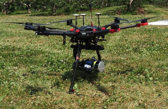
Remote Sens. 2020, 12, 2806 3 of 17
were used and stress the importance of GCP use for accurate DSM production, as reiterated in other
studies [30–33]. Wallace et al. [34] compared UAS imagery to airborne LiDAR to assess forest structure.
They discovered that
Remote Sens. 2020, 12, while UAS
x FOR PEER DSMs were not as accurate as DSMs produced from airborne
REVIEW LiDAR,
3 of 18
they were a sufficient low-cost alternative for surveying forest stands but lacked detail compared
to LiDARbetween datasets Because
products. when GCPs of were
theseused and stress theinimportance
advancements of GCP use
UAS technology, for accurate
sensors, DSM
and processing
production, as reiterated in other studies [30–33]. Wallace et al. [34] compared UAS imagery to
techniques, geographic data can be collected at lower altitudes, higher resolutions, and user-defined
airborne LiDAR to assess forest structure. They discovered that while UAS DSMs were not as
spatialaccurate
and temporal scales. Thus, many researchers are testing the practical applications of these
as DSMs produced from airborne LiDAR, they were a sufficient low-cost alternative for
capabilities
surveying[35]. forest stands but lacked detail compared to LiDAR products. Because of these
Flight control and
advancements in UASstabilization
technology, systems,
sensors,through the integration
and processing techniques, of geographic
Global Navigation
data can Satellite
be
System (GNSS)
collected receivers
at lower and higher
altitudes, Inertial Measurement
resolutions, Units (IMUs),
and user-defined spatial have facilitated
and temporal the
scales. addition
Thus,
of LiDARmanysensors
researchers onare testing
UAS. the can
This practical applications
be more of these capabilities
cost efficient [35].
than traditional airborne LiDAR for
local-scale investigations. In recent years, UAS-LiDAR has been tested inNavigation
Flight control and stabilization systems, through the integration of Global a multitudeSatellite
of fields
System (GNSS) receivers and Inertial Measurement Units (IMUs), have facilitated the addition of
including ecology [36], forestry [37–40] and precision agriculture [41], predominantly for vegetation
LiDAR sensors on UAS. This can be more cost efficient than traditional airborne LiDAR for local-
mapping [42]. Results in each case showed that UAS-LiDAR produced high-quality, reliable results
scale investigations. In recent years, UAS-LiDAR has been tested in a multitude of fields including
when ecology
compared [36],toforestry
airborne LiDAR
[37–40] and sources.
precision Several different
agriculture LiDAR models
[41], predominantly are available
for vegetation for use on
mapping
UAS and [42].are introduced
Results in each in casetheshowed
study that
by Giordan
UAS-LiDAR et al.produced
[42]. Here, we focusreliable
high-quality, on the results
Velodyne when VLP-16
Puck Lite model,
compared to which
airborne was
LiDARcommon
sources. at Several
the time of dataLiDAR
different collection.
models are available for use on UAS
Inand
thisare introduced
study, we use inphotogrammetry
the study by Giordan andethigh-precision
al. [42]. Here, weGCPsfocus tooncreate
the Velodyne VLP-16
DSMs from Puck
four popular
Lite model, which was common at the time of data collection.
UAS (DJI Inspire 1, DJI Phantom 4 Pro, DJI Mavic Pro, and DJI Matrice 210) to compare the results of
commonlyInpurchased
this study, we use photogrammetry and high-precision GCPs to create DSMs from four
platforms. The accuracy and spatial variability of these DSMs will be compared
popular UAS (DJI Inspire 1, DJI Phantom 4 Pro, DJI Mavic Pro, and DJI Matrice 210) to compare the
to (1) 12 high-precision GPS targets (checkpoints) in the field to quantify overall vertical accuracy,
results of commonly purchased platforms. The accuracy and spatial variability of these DSMs will be
and (2)compared
a DSM created
to (1) 12from Light Detection
high-precision and(checkpoints)
GPS targets Ranging (LiDAR) (Velodyne
in the field VLP-16
to quantify Puck
overall Lite) on a
vertical
fifth UAS,
accuracy, and (2) a DSM created from Light Detection and Ranging (LiDAR) (Velodyne VLP-16 Puck was
a DJI Matrice 600 Pro, to investigate spatial errors across the study area. This research
designedLite)toonquantify howa DSMs
a fifth UAS, generated
DJI Matrice from
600 Pro, multiple UAS
to investigate differ,
spatial errorsand to identify
across the studyand
area.characterize
This
research
differences was space
across designed andtoland
quantify
cover how DSMs
types in generated from multiple
a single study area. UAS differ, and to identify
and characterize differences across space and land cover types in a single study area.
2. Materials and Methods
2. Materials and Methods
2.1. Study Site
2.1. Study Site
The study site, located at 44◦ 560 55”N, 65◦ 070 13”W near Middleton, Nova Scotia (NS), Canada
(Figure 2),The
wasstudy site, due
chosen located
to at
its44°56′55″N,
mixed land 65°07′13″W near Middleton,
cover features, Nova
including Scotiabare
vines, (NS),soil,
Canada
dirt road,
(Figure 2), was chosen due to its mixed land cover features, including vines, bare
long grass, mowed grass, and forest. The site was approximately eight hectares (~20 acres) soil, dirt road, longin area
grass, mowed grass, and forest. The site was approximately eight hectares (~20 acres) in area which
which enabled each flight to be conducted on a single battery (approximately 15 min flying time).
enabled each flight to be conducted on a single battery (approximately 15 min flying time).
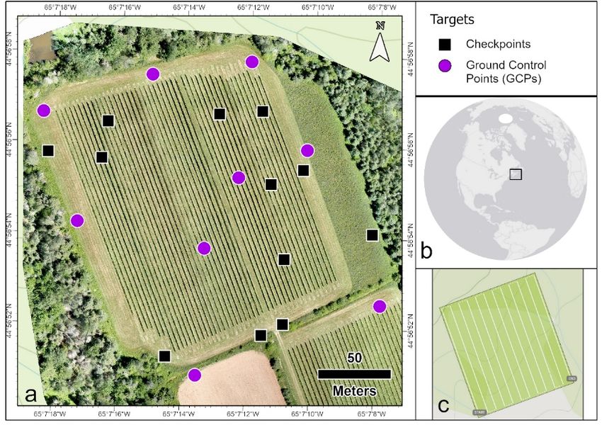
FigureFigure 2. Aerial
2. Aerial mapmap (a) study
(a) of of study areanear
area nearMiddleton,
Middleton, Nova
NovaScotia,
Scotia,Canada, (b) with
Canada, distribution
(b) with of
distribution of
21 targets: 12 checkpoints as purple circles and nine Ground Control Points (GCPs) as black squares.
21 targets: 12 checkpoints as purple circles and nine Ground Control Points (GCPs) as black squares.
Flights were flown in a grid pattern (c) from 70 m elevation.
Flights were flown in a grid pattern (c) from 70 m elevation.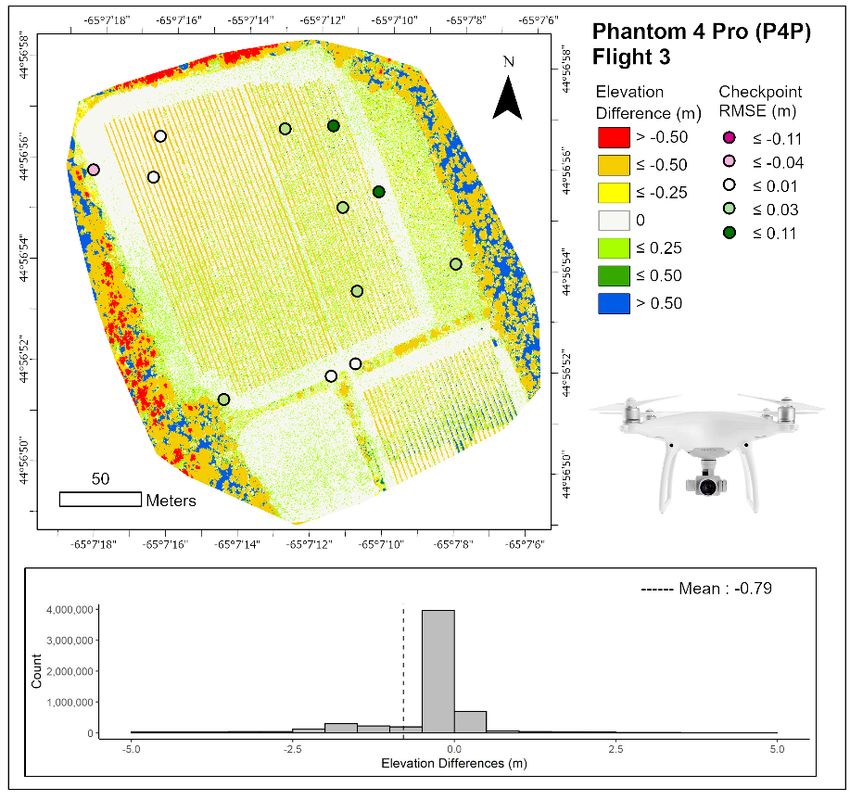
Remote Sens. 2020, 12, 2806                                                                            4 of 17

2.2. Ground Control Points (GCPs) and Checkpoints
     Twenty-one (21) targets were spread across the study area (Figure 2); nine Aeropoint™ targets
with integrated GPS were used as GCPs for georectifying the UAS imagery (Section 2.5). Additionally,
12 checkpoints in the form of 20 × 20 wooden targets, painted in a black-and-white checkerboard pattern,
were spread across the study area. The Aeropoint targets were used to reference the model (GCPs) and
the remaining targets were retained for validating model accuracy (checkpoints). The location of each
target was logged using a Leica RTK GPS 1200 survey-grade GNSS receiver (1 cm accuracy). All GPS
data were post-processed using data from the Nova Scotia Active Control System station (NSACS)
number NS250002 [43] in Lawrencetown, NS, which was approximately eight kilometers away from
the study site. Locations of Aeropoint targets were processed using the Aeropoints cloud-based system
and Leica GPS locations were post-processed using Leica GeoOffice.

2.3. Creation of the UAS-LiDAR Dataset
      A DJI Matrice 600 Pro UAS equipped with a Velodyne VLP-16 LiDAR sensor and an Applanix
APX-15 UAS IMU (Table 1, Figure 3) was used to create the UAS-LiDAR dataset, henceforth referred to
as LiDAR. The assembled system weighed approximately 11 kg, had a diameter of 170 cm, a maximum
speed of 65 km/h, and a flight time of approximately 16 min. Six batteries are required to propel this
unit. The LiDAR flight was flown on 20 July 2018 prior to the UAS flights described in Section 2.4.
For our mission, the LiDAR was flown at a speed of 10 m/s from 70 m elevation (above ground level)
with 50 m strip spacing and 150,000 pulses/second at 180◦ field of view. The systems captured two
returns—the strongest and the last. Post-flight IMU trajectory data were processed using POSPac
UAV [44]. GPS base station log files were downloaded from the NSACS station number NS250002 [43].
Data from the IMU and the base station were blended to calculate the aircraft trajectory, stored in
Smoothed Best Estimate of Trajectory (SBET) files. Laser returns were downloaded from the LiDAR
sensor and processed with the IMU trajectory file in Phoenix Spatial Explorer [45] to create a point cloud
dataset. The LiDAR Data Exchange Format (LAS) point cloud data were cleaned using the Statistical
Outlier Removal tool in CloudCompare [46] and systematic point data representing point reflections
from the legs of the UAS were removed. LiDAR data were analyzed against the survey-grade GPS
measurements of elevation from GCPs (Section 2.2) to obtain accuracy values. After verifying the
LiDAR data against the 12 checkpoints, the LiDAR had a vertical Root Mean Square Error (RMSE)
of ±0.04 m, a mean error (ME) of ±0.03 m, and standard deviation (St. Dev.) of ±0.02 m (Table 2).
According to standards developed by the Federal Geographic Data Committee [47] and reported by
Evans et al. [48], ±0.04 m is an acceptable vertical error value for LiDAR used in terrain and land
cover mapping and was deemed suitable for comparison of UAS DSMs in this study. The LAS file
was converted to a raster in ArcGIS Pro 2.1 [49] to create the LiDAR DSM using the LAS Dataset to
Raster tool. Before conversion, the LiDAR point cloud density was 343 pts/m2 . The triangulation
interpolation method was used, and the maximum point value was assigned to each cell in the output
raster, representing the top surface of the terrain to creating the DSM. The void fill method was set
to linear. Output cell size was 0.10 m and was selected as it provided sufficient detail to distinguish
between land cover types and give an accurate representation of the terrain without slowing down
processing times.
        Table 1. Specifications of UAS with LiDAR and IMU. GNSS: Global Navigation Satellite System.

                  Unit                   Specification                          Value
                                          Weight (kg)                             10
                                        Diameter (cm)                            170
                                    Max. takeoff weight (kg)                     15.5
                                      Max. payload (kg)                           5.5
        DJI Matrice 600 Pro UAS
                                      Max. speed (km/h)                           65
                                    Max. hover time (min)                         16
                                      Manufacture year                           2017
                                            Cost *                           ~30,000 USD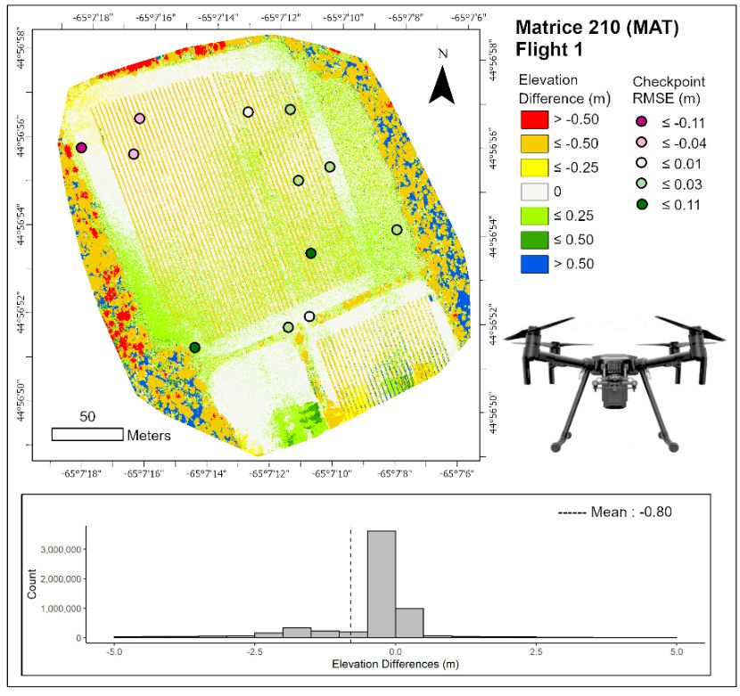
Remote Sens. 2020, 12, 2806 5 of 17
Table 1. Cont.
Remote Unit
Sens. 2020, 12, x FOR PEER REVIEW Specification Value 5 of 18
Weight (g) 830
Cost * ~30,000 USD
No. of returns 2 (strongest and last)
Velodyne VLP-16 LiDAR Weight (g) 830
Accuracy (m) ±0.03
No. of returns 2 (strongest and last)
Beam divergence (degrees) 0.16875
Accuracy (m) ±0.03
Points/second Up to 600,000
Velodyne VLP-16 LiDAR Beam divergence (degrees) 0.16875
No. of lasers 16
Points/second Up to 600,000
Laser wavelength (nm) 903
No. of lasers 16
Laser range (m) 100
Laser wavelength (nm) 903
Field of view (degrees) 360
Laser range (m) 100
Manufacture year 2018
Field of view (degrees) 360
Cost * ~20,000 USD
Manufacture year 2018
Weight
Cost * (g) ~20,000 USD 60
Applanix APX-15 IMU No. ofWeight
possible
(g)satellites 336
60 GNSS channels
Rate
No.ofof data collection
possible (Hz)
satellites 336 GNSS channels 200
Applanix APX-15 IMU
Parameters
Rate of data collection (Hz) Position, Time,200Velocity, Heading, Pitch, Roll
Manufacture
Parameters year 2017 Pitch, Roll
Position, Time, Velocity, Heading,
Cost * year
Manufacture 2017~15,000 USD
Cost * ~15,000 USD
* Costs are approximate, as the whole system was purchased as one unit, with educational discounts applied.
* Costs
Further, costs haveare approximate,
decreased sinceasthis
the study
whole system was purchased as one unit, with educational discounts
was conducted.
applied. Further, costs have decreased since this study was conducted.
Figure 3. Image of DJI Matrice 600 Pro with Velodyne Puck mounted and pointed at nadir.
Figure 3. Image of DJI Matrice 600 Pro with Velodyne Puck mounted and pointed at nadir.
Table 2. Locations of checkpoints (CPs) in decimal degrees, altitude (m) of each checkpoint, and
Table 2. Locations of checkpoints (CPs) in decimal degrees, altitude (m) of each checkpoint,
differences between LiDAR DSMs and checkpoints in meters (m). Overall Mean Error (ME), Standard
and differences between
Deviation LiDAR
of Error (St. DSMs
Dev.), Mean and checkpoints
Average in RMSE
Error (MAE), and meters
also(m).
listed.Overall Mean Error (ME),
Standard Deviation of Error (St. Dev.), Mean Average Error (MAE), and RMSE also listed.
CP Longitude Latitude Altitude LiDAR
CP P1 −65.11892131
Longitude 44.94836999
Latitude 54.75 Altitude
0.03 LiDAR
P2 −65.11953122 44.94875508 61.09 0.05
P1 −65.11892131 44.94836999 54.75 0.03
P3 −65.1196785 44.9482073 59.96 0.03
P2 −65.11953122 44.94875508 61.09 0.05
P3 P4 −65.11980599
−65.1196785 44.94866469
44.9482073 63.44 0.05
59.96 0.03
P4 P5 −65.11989563
−65.11980599 44.94911118
44.94866469 63.24 0.05
63.44 0.05
P5 P6 −65.11986297
−65.11989563 44.94773879
44.94911118 57.41 0.01
63.24 0.05
P6 P7 −65.12068701
−65.11986297 44.94759533
44.94773879 57.64 0.08
57.41 0.01
P7 P9 −65.12173866
−65.12068701 44.94883572
44.94759533 72.04 0.02
57.64 0.08
P9 −65.12173866
P10 −65.1212735 44.94883572
44.94880432 71.54 72.04
−0.02 0.02
P10 −65.1212735
P11 −65.12122784 44.94880432
44.94902887 72.39 71.54
0.03 −0.02
P11 −65.12122784
P12 −65.12026788 44.94902887
44.94908824 66.85 72.39
0.04 0.03
P12 −65.12026788 44.94908824 66.85 0.04
P20 −65.11967805 44.94780874 57.09 0.01
ME 0.03
St. Dev. 0.02
MAE 0.04
RMSE 0.04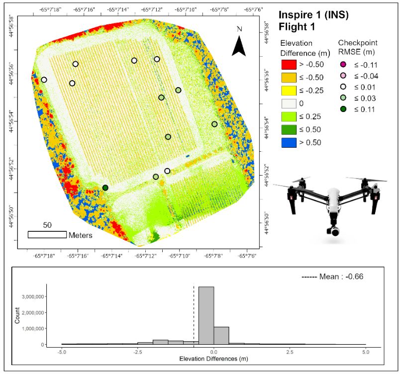
Remote Sens.Remote Sens.Remote
2020,Sens.
Remote 12, x 2020, Sens.
2020, 12,
FOR PEER 2020,PEER
x FOR
REVIEW
12, x FOR 12, x REVIEW
FOR PEER REVIEW
PEER REVIEW 6 of 186 of 186 of 18
6 of 18
Remote Sens. 2020, 12, 2806 6 of 17
P20 P20 P20
−65.11967805
P20 −65.11967805
−65.11967805 44.94780874
44.94780874
44.94780874
−65.11967805 57.0957.0957.09
44.94780874 57.09
0.01 0.01 0.01 0.01
ME ME ME 0.03ME
0.03 0.03 0.03
2.4. UAS Imagery—Data Collection St. Dev.
St. Dev. St. Dev.
0.02
St. Dev. 0.02 0.02 0.02
MAE MAEMAE MAE
0.04 0.04 0.04 0.04
The four UAS used in this study were Dà-Jiāng Innovations RMSE
(DJI)0.04
RMSE
Inspire
RMSE 1 V1 (INS),
0.04 0.04 0.04
DJI Matrice
RMSE
210 (MAT), DJI Mavic Pro (MAV), and the DJI Phantom 4 Professional (P4P). Each was flown three
times in random 2.4.sequence
2.4. UAS UAS
2.4. 2.4. UAS
Imagery—Data
Imagery—Data
UAS over Imagery—Data
theCollection
Collection
Imagery—Data study Collection
area and each carried a different high-resolution RGB sensor
Collection
(Table 3). A full Thebattery
The
fourfour
UAS
The was
The
UAS
used
four UASused
four
used UAS
in this
used for
used
in this each
in study
study instudy
were
this thisflight.
were study
Dà-Jiāng
Dà-Jiāng
were Flights
were
Dà-JiāngDà-Jiāng were
Innovations
Innovations (DJI)
Innovations planned
Innovations
(DJI) Inspire
Inspire
(DJI) V1with
1(DJI) Inspire
1(INS),
Inspire V1 the
1(INS),
V1 DJI Pix4D
1 V1
DJI(INS),
Matrice
Matrice
(INS), Capture
DJI Matrice
DJI Matrice
application 210
using210
(MAT),a(MAT),
210 210Mavic
DJI
(MAT),
grid (MAT),
DJI
patternMavic
DJIPro DJIProMavic
(MAV),
Mavic
(Figure (MAV),
Pro and Proand
(MAV),
2c); (MAV),
the DJI
and
identical andPhantom
the Phantom
DJI
the DJIthePhantom
plans DJI Phantom
4 Professional
4 Professional
were 4 used 4 (P4P).
Professional
for(P4P).
Professional Each
each Each(P4P).
was
(P4P). was
flown
Each
flight. Each
flown
was
All was
three
flown flown
three
flights threethree
were
timestimes
intimes
randomtimes
in random sequence over the study area and each carried a different high-resolution RGB RGB
in random in random
sequence
sequence over sequence
over
the the
study over
studyareathe
areastudy
and and
each area
each and
carried
carried each
a a carried
different
different a different high-resolution
high-resolution
high-resolution RGB RGB
flown at an altitude of sensor 70 m (Table
with 70% 3). front andwas side overlap and the camera angle atwith
nadir. WhileCapture
70%
sensor
sensor (Table (Table
sensor A3).
3).(Table A3).
full full fullA
A battery
battery wasfull
wasbattery
used
battery used
wasfor used
each used
for each
flight.
for for
flight.
each each
Flights
flight. flight.
Flights
were
Flights Flights
were
planned
were were
plannedplannedplanned
withwith the Pix4D
the with
Pix4D the the
Capture
Pix4D Pix4D
CaptureCapture
is the minimum recommended
application
application application
using
application using
a grida grid
using front
using
pattern
a grid a
patternoverlap
grid
(Figure
pattern pattern
(Figure
2c); for photogrammetric
(Figure
2c); identical
identical
(Figure 2c);
plans
2c); identical identical
plans
were were
plans plans
used used
were surveys,
were used
for each
for used
each this
for
flight.
flight.
for each All value
each ensured
flight.
All flights
flights
flight. AllwereAll
flights that
werewerewere
flights
we would be able
flown flown at an altitude of 70 m with 70% front and side overlap and the camera angle at nadir.nadir.
atto
flown an at flown
cover
an at
the
altitude
altitude of an70 altitude
entire
ofm 70 m
with of
study
with
70% 70 m
area
70%
frontwith on
front
and 70%one
and
side front
side
overlapand
battery
overlapside
andfor overlap
and
theeach
the
camera and
camera the
platform.
angle camera
angle
at at angle
Respective
nadir.
nadir. While at
While WhileWhile
Ground
70% 70%
is theis
70% the70%
minimum
is the isminimum
minimum the minimum
recommended
recommended recommended
recommendedfront front
overlap
front front
overlapfor overlap
for
photogrammetric
overlap for for photogrammetric
photogrammetric
photogrammetric surveys,
surveys, this surveys,
this
value
surveys, value this
ensured
this value value
ensuredensuredensured
Sampling Distances (GSDs) are listed in Table 2. Data were collected on July 20, 2018 over a span of
thatthat
we thatwould that
we would
we be we bewould
able
would able
to tobecover
becover
able able to cover
the
thecover
to entire entire
thestudy the
entire entire
study
area
study onstudy
area on one
one
area area
battery
on one onfor
batteryoneeach
battery battery
for each for each
platform.
platform.
for each platform.
Respective
Respective
platform. Respective
Respective
approximately 3.5
Ground
Ground
h fromGround10:00
Sampling
Sampling
to
Sampling13:30
Distances
Distances (GSDs)
AST
Distances
(GSDs)are
toare
avoid
(GSDs)
listed listed
shadows.
are listed
in Table
in listed
Table 2. Table
Data
The
2.inData
Table
were
weather
2. Data
were were
collected
collected
conditions
collected
on July
on July 20, 20,
were
on2018
July2018consistent
20,
a 2018
over a over a
Ground Sampling Distances (GSDs) are in 2. Data were collected on 2018
July over
20, over a
for the duration ofofapproximately
spanspan the
of
span day,
span
of ofsun
approximately 3.5with
approximately
approximately h3.5
from no
h3.5
fromhcloud
3.5
10:00 h from
10:00
fromto cover
to
13:30
10:00 10:00
13:30
AST and
AST
to
to 13:30 noavoid
to avoid
13:30
to
AST wind.
AST
to to avoid
shadows.
shadows.
avoid Theshadows.
shadows.The weather
weather
The Theconditions
weather
conditions
weather conditions
were werewerewere
conditions
consistent forconsistent
consistent the
consistent forduration
for duration
the the thethe
forduration
of duration
of day,
the ofday,
ofday,
sun
the the with
sun
withday, sun
no cloud
sun with with
no cloud
no no cloud
cover
cover and
cloud no cover
and
cover and
no wind.
wind.
and no no wind.
wind.
Table 3. Specifications of UAS. All produced by Dà-Jiāng Innovations (DJI). No. batteries: number of
TableTable Table
3. Specifications
Table 3. of
Specifications
3. Specifications of UAS.
UAS.
3. Specifications All ofproduced
All UAS.
produced
of UAS. AllDà-Jiāng
by produced
by
All produced Dà-JiāngbyInnovations
Dà-Jiāng
Innovations
by Dà-Jiāng Innovations
(DJI).
(DJI).
Innovations (DJI). No.number
No. batteries:
No.(DJI).
batteries: numberbatteries:
No. batteries:of ofnumber
number of of
batteries required to operate.
batteries
GSD:
required
Ground
to
Sampling
operate. GSD:
Distance
Ground Sampling
(from 70 m
Distance
altitude);
(from 70 m
GNSS:
altitude);
Global
GNSS: Global
batteries
batteries required
required to to operate.
operate. GSD: GSD: Ground
Ground Sampling
Sampling Distance
Distance (from(from
70 m70 m altitude);
altitude); GNSS:
batteries required to operate. GSD: Ground Sampling Distance (from 70 m altitude); GNSS: Global GNSS: Global
Global
Navigation Navigation
Satellite System;
NavigationSatellite
Navigation
GPS:
Navigation
Satellite Global
System;
Satellite GPS:Positioning
Satellite
System;
System;System;
GPS: GPS:
Global
Global
GPS:
Systems
Global
Positioning
Positioning
Global
(United
Positioning
Systems
Systems
Positioning
States);
Systems
(United
(United
Systems
GLONASS:
(United
States);
States);
(United
Global’naya
States);
GLONASS:
GLONASS:
States); GLONASS:
GLONASS:
Navigatsionnaya Sputnikovaya
Global’naya
Global’naya Global’naya
Navigatsionnaya
Global’naya Sistema (Russia).
Navigatsionnaya
Navigatsionnaya Sputnikovaya
Sputnikovaya
Navigatsionnaya Sputnikovaya
Sistema Sistema
(Russia).
Sistema (Russia).
Sputnikovaya (Russia).
Sistema (Russia).
Matrice
Matrice 210 210Matrice
Matrice 210 210 Phantom
Phantom Phantom
Pro4 Pro
4Phantom 4 Pro 4 Pro
Inspire
Inspire
Inspire11 V1
V1 V1Inspire
1(INS)
Inspire (INS)
(INS) 1Matrice
V1 (INS) 210 (MAT)
1 V1 (INS) Mavic
Mavic
(MAT) Mavic
Pro (MAV)
Mavic Mavic
Pro (MAV)
Pro Pro (MAV) Phantom 4 Pro (P4P)
(MAV)
Pro (MAV) (P4P)
(MAT)(MAT) (MAT) (P4P)(P4P) (P4P)
Platform Platform
Platform Platform
Platform
(cm)Dimensions
Dimensions Dimensions (cm)Dimensions
(cm)
Dimensions 43.7
(cm) (cm)
43.7××43.7
30.2×43.7
30.2 30.2
×× ××43.7
45.3
45.3 45.3×× 88.7
30.2 30.2
88.7
45.3 ××88.7
45.3
××88.7
88.0 ×88.0 ×××
37.8
88.0 88.7
37.8×× 88.0
37.8
88.0 19.8××19.8
37.8 37.8 ×19.8 19.8
8.3××× 8.3
8.319.8 8.3 ××
8.3 ×25.0
8.3
8.3××25.0
8.3 8.3 ×25.0
25.0 ×25.0××25.0
20.0
25.0 ×××25.0
20.0
25.0 25.0
20.0 ××20.0
20.0
Weight (g) Weight Weight (g) Weight
(g)Weight (g)
(g) 30603060 3060
~
~
3060 ~ 3060 45704570
~ ~
4570 4570 4570 734 734 734 734 734 1388 1388 1388 1388 1388
Max Max
FlightFlight
Time
Max Max Flight
Time
Flight Time Time
Max Flight Time (min) 18
18 18 18 18 38 38 38 38 38 27 27 27 27 27 30 30 30 30
30
(min)(min)(min) (min)
No. Batteries No. Batteries
No. Batteries No. Batteries11 1 1 2
22 2 1 1 1 1 1 1 11
No. Batteries 1 2 1 1
Sensor (CMOS) Sensor
Sensor (CMOS) Sensor
(CMOS)
Sensor (CMOS) 1/2.3”
1/2.3″1/2.3″1/2.3″ 1/2.3″ 4/3″ 4/3”
(CMOS) 4/3″ 4/3″ 4/3″ 1/2.3″1/2.3″1/2.3” 1/2.3″ 1/2.3″ 1″ 1″ 1″ 1”
1″
Effective PixelsEffective
(MP) Effective
Pixels Effective
Pixels
Effective 12.4
Pixels Pixels 20.8 ˆ 12.35 20
12.4 12.4 12.4 12.4 20.8 ^20.8 ^20.8 ^ 20.8 ^ 12.3512.35 12.35 12.35 20 20 20 20
GSD—70 m (cm/px) (MP)(MP) (MP) (MP) 3.06 1.55 2.3 1.91
GNSS GSD—70 GSD—70m mGSD—70
GSD—70 GPS m
m + GLONASS GPS1.55
3.06 + GLONASS GPS2.3+ GLONASS GPS + GLONASS
(cm/px) 3.06 3.06 3.06 1.55 1.55 1.55 2.3 2.3 2.3 1.91 1.91 1.91 1.91
(cm/px)
(cm/px)
GNSS Vertical Accuracy (m) (cm/px) +/- 0.5 +/- 0.5 * +/- 0.5 +/- 0.5
GNSSGNSSGNSS GNSS GPS +GPS +GPS
GLONASS + GPS
GLONASS +GPS
GLONASS GLONASS
+GPS +GPS
GLONASS + GPS
GLONASS +GPS
GLONASS GLONASS
+GPS +GPS + GPS
GLONASS
GLONASS + GPS
GLONASS GLONASS
+GPS +GPS + GPS
GLONASS
GLONASS + GLONASS
GLONASS
GNSS Horizontal Accuracy (m) GNSS +/- 2.5
Vertical +/- 1.5 * +/- 1.5 +/- 1.5
GNSSGNSS Vertical
Vertical
GNSS Vertical
Manufacture Year Accuracy +/- 0.5+/- 0.5+/- 0.5 +/- 0.5+/- 0.5+/-
2014 * 0.5 +/-
* 0.5+/-
2017 * 0.5 +/-
* 0.5+/- 0.5+/-
2017 0.5 +/- 0.5+/- 0.5+/- 0.5+/- 0.5 +/-
2016 0.5
Accuracy
Accuracy (m) (m)
Accuracy (m) (m)
Cost GNSSGNSS GNSS
Horizontal
Horizontal
GNSS ~2000
Horizontal
Horizontal USD ~7000 USD ~1000 USD ~1500 USD
+/- 2.5+/- 2.5+/- 2.5 +/- 2.5+/- 1.5+/-* 1.5+/-
Accuracy (m) * 1.5 +/-
* 1.5 +/-
* 1.5+/- 1.5+/- 1.5 +/- 1.5+/- 1.5+/- 1.5+/- 1.5 +/- 1.5
~ Accuracy (m)
Accuracy (m)
Accuracy (m)
With Zenmus X3; * Accuracy increases
Manufacture Year with Downward
2014 Vision System
2017 Enabled; ˆ Zenmuse
2017 X5S add 2016
on.
Manufacture
Manufacture Year Year Year 2014 2014 2014
Manufacture 2017 2017 2017 2017 2017 2017 2016 2016 2016
Cost Cost Cost Cost~2000~2000 USD ~2000
USD~2000 USD~7000
USD ~7000 USD~7000USD ~7000 USD~1000
USD ~1000 USD ~1000
USD~1000 USD ~1500
USD ~1500 USD ~1500
USD~1500 USD USD
2.5. UAS Imagery—Data
~ With
~ With Zenmus ~Processing
~ With With
Zenmus
X3;
ZenmusZenmus
*X3; * X3;
Accuracy *Workflow
X3;
Accuracy * increases
Accuracy
increases
Accuracy increases
withwith
Downward
increases with with
Downward Downward
Vision
Vision
Downward System Vision
System System
Enabled;
Enabled;
Vision System ^Enabled;
X5S^ add
Zenmuse
^ Zenmuse
Enabled; Zenmuse
X5S
^ Zenmuse add X5Son.
X5S on.
on. add add on.
Aerial 2.5.
images
2.5. UAS
UAS from
2.5. 2.5. each
UAS
Imagery—Data
Imagery—Data
UAS UAS
Imagery—Dataflight
Processing
Processing
Imagery—Data were
Processing
Workflow
Workflow
Processing processed
Workflow in the photogrammetric image processing
Workflow
software Agisoft Metashape Aerial (Version
images 1.2.6
from each Build
UAS 2934)
flight [16]
were according
in processed theto theimage
USGS-recommended
AerialAerial
imagesimages
Aerial from from
images each each
fromUAS UAS
flight
each flight
UAS were were processed
processed
flight were the
processed theinphotogrammetric
in photogrammetric
the photogrammetric
in photogrammetric image image
processing
processing
image processing
processing
workflow [50]. Each
software
software dataset
software
Agisoft
Agisoft was aligned
Agisoft
Metashape
Metashape using
Metashape
(Version
(Version 1.2.6 a
1.2.6high-accuracy
(Version
BuildBuild 1.2.6
2934) Build
2934)
[16] [16] alignment
2934) [16]
according
according
software Agisoft Metashape (Version 1.2.6 Build 2934) [16] according to the USGS-recommended to to
the (full
according
the image
to the resolution)
USGS-recommended
USGS-recommended
USGS-recommended with
system defaults
workflow key
workflow workflow
forworkflow
[50]. point
[50].
Each and
Each
[50]. [50]. Each
tie-point
dataset
dataset
Each was was
dataset dataset
aligned
aligned
was wasusing
limits
using
alignedaligned
(50,000; using a high-accuracy
a10,000).
a high-accuracy
a high-accuracy
using Then,
alignment
alignment
high-accuracy thealignment
(full
alignment nine
(full
imageimage (full
Aeropoint image
resolution)
resolution)
(full image resolution)
GCP
with
resolution) with with
withtargets
system
system system
defaults
defaults for defaults
for key for
point key
and point and
tie-point tie-point
limits limits
(50,000; (50,000;
10,000). 10,000).
Then, the Then,
nine the nine
Aeropoint Aeropoint
GCPGCP GCP
were manually system
identified inkey
defaults point
for key
photos and
and tie-point
point and
assigned limits
tie-point (50,000;
limits
survey-grade 10,000).
(50,000; Then,
10,000).
geographic the nine
Then, Aeropoint
the nine
coordinates. GCP
Aeropoint
Dense point
targets
targets were targets
were
manually were
manually manually
identified
identified in identified
in
photosphotos
and in photos
and assigned
assigned and assigned
survey-grade
survey-grade survey-grade
geographic
geographic
targets were manually identified in photos and assigned survey-grade geographic coordinates. Dense geographic
coordinates.
coordinates. coordinates.
DenseDense Dense
clouds werepoint
created atpoint
the high-quality
clouds were setting
atcreated theand were exported in LAS format. Respective point
point clouds
clouds
point were were
clouds created
created
were at the
created the theathigh-quality
at high-quality
high-quality high-quality
setting
setting and andsetting
were
setting were and
exported
and were were
exported exported
in LAS
exportedin LAS
format.
in LAS in Respective
LAS
format. format.
Respective
format. Respective
Respective
cloud densities
point are
point listed
cloud
point point
cloud in
densities
cloud Table
cloud
densities 3. Each
densities
are listed
are listed
densities are are LAS
listed
in Table
in listed
Table in dataset
in Table
3. Each
3. Each
Table LAS LASwas
3. Each converted
dataset
dataset
3. Each LAS LAS
was dataset
was to
converted
converted
dataset was a
was DSM
converted
to a to
converted DSM with
a DSM
towith to the
a
with
a DSM DSMLASwith
the LAS
the with
LAS to Raster
the
to to
to LAS
the LAS to
tool in ArcGIS Pro, using triangulation as the interpolation technique, with the points of maximum
elevation. Each output DSM was produced with a resolution of 0.10 m to remain consistent with the
output LiDAR DSM and to obtain sufficient detail for distinguishing between land cover types while
accurately representing the elevation changes across the site and keeping processing times manageable.
Orthophoto mosaics were also created from each dense point cloud. Land covers across the study
area were manually delineated from an orthophoto mosaic produced from the INS UAS. Land cover
was differentiated into six different land cover categories: vines, bare soil, dirt road, mowed grass,
long grass and forest.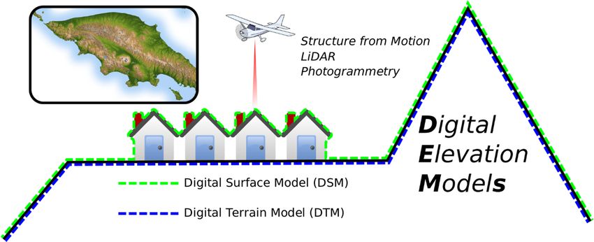
Remote Sens. 2020, 12, 2806                                                                                             7 of 17

2.6. Creation of DSMs of Difference (DoDs)
      DSMs of Difference (DoDs) were used to compare the DSMs from the UAS against those from
LiDAR and visualize spatial differences across the study area. To create DoDs, the LiDAR DSM was
subtracted from each UAS DSM in ArcGIS Pro [49]. This created a difference raster for each dataset,
where each pixel represented the vertical difference between the aerial image-derived DSM (from
UAS) and the LiDAR DSM. These DoD rasters were used to generate four different standard accuracy
statistics: ME, St. Dev., Mean Average Error (MAE) and RMSE. ME represents an average of all
errors across the DoDs while the St. Dev. measures the error variability. RMSE and MAE scores are
interpreted in measured units and do not account for direction of error. However, RMSE is more
sensitive to larger errors and increases when variance in error is high. MAE is easier to interpret,
showing the average, absolute difference between predicted and measured values. DoDs enabled the
visualization of spatial differences between the two data collection methods across the study area [51].

3. Results
3.1. Accuracy of UAS DSMs Compared to Checkpoints and DSMs of Difference (DoDs)
      The details of each UAS flight including start time, order, duration, number of images, resulting
point cloud density, and statistics of output DSMs compared to 12 checkpoints are listed in Table 4.
Based on these results, the best flight was chosen for each platform (shown in bold) and elaborated in
the sections below. We determined the best flights to be those with the lowest error values overall.
Locations of checkpoints are shown in Figure 2 and associated error values for each checkpoint are
listed in Supplementary Table S1 (Table S1). DoDs were created by subtracting the LiDAR DSM from
each UAS DSM to determine where spatial differences occurred across the study area. These statistics
are listed in Table 5 and shown in Figures 4–7.
      Table 4. Detailed flight information for each UAS flight. Error statistics represent overall differences
      compared to 12 checkpoints across the study site. All times in Atlantic Standard Time (AST). The
      bolded flight indicates the best flight selected for further analysis. ME: Mean Error; St. Dev.: Standard
      Deviation of Error; MAE: Mean Average Error; RMSE: Root Mean Square Error. All errors reported in
      meters (m). Point cloud density shown in points per square meter (pts/m2 ).

                        Flight Start      Flight                   No.      Point Cloud
    UAS      Flight #                              Duration                               ME       St. Dev.   MAE RMSE
                           Time           Order                  Images       Density
                1             10:15            2   9 min 32 s      117        434.03      0.01       0.03     0.02   0.03
     INS        2             11:50            7   9 min 36 s      117        452.69      0.02       0.03     0.02   0.03
                3             12:45           11   9 min 30 s      117        434.03      0.02       0.02     0.03   0.03
                1             10:50            4   11 min 6 s      216        1371.70     0.003      0.07     0.05   0.06
    MAT         2             11:35            6   9 min 42 s      160        1275.51     −0.03      0.25     0.11   0.24
                3             12:30           10   9 min 43 s      160        1371.74     0.02       0.08     0.07   0.08
                1             10:30           3    12 min 5 s      177        771.60      0.04       0.05     0.05   0.06
    MAV         2             12:00           8    11 min 34 s     176        730.60      0.04       0.05     0.05   0.07
                3             12:15           9    11 min 54 s     176        730.46      0.05       0.06     0.05   0.07
                1             10:00            1    8 min 10 s     146        1111.11     0.02       0.03     0.03   0.04
     P4P        2             11:17            5   10 min 35 s     160        1040.58     0.01       0.03     0.03   0.04
                3             13:00           12   10 min 36 s     160        1040.58     0.007      0.03     0.02   0.03

      Table 5. Overall error statistics of DSMs of Difference (DoDs) between the LiDAR dataset and four
      UAS. ME: Mean Error, St. Dev.: Standard Deviation of Error, MAE: Mean Average Error, RMSE: Root
      Mean Square Error. All errors reported in meters (m).

                              UAS and Flight #       ME          St. Dev.      MAE        RMSE
                                      INS 1          −0.66         2.37         0.95        2.09
                                      MAT 1          −0.80         2.43         1.02        1.97
                                      MAV 1          −0.64         2.33         0.94        2.03
                                      P4P 3          −0.79         2.58         1.03        2.04
Compared to the LiDAR DSM, the INS DoD had the second lowest ME (−0.66 m), St. Dev. (2.37
m), and MAE (0.95 m) (Table 5). The overall RMSE for this flight was highest at 2.09 m. The high St.
Dev. value indicates that there are inconsistencies in error across the study site while the negative
mean error value indicates that the INS DSM consistently underestimates elevation. As seen in the
spatial errors across the DoD for the INS platform (Figure 4), the lowest error values are seen on non-
Remote Sens. 2020, 12,
vegetated 2806 while the highest errors are in areas covered by vegetation—in this case, forest and 8 of 17
terrain,
vines.
Remote Sens. 2020, 12, x FOR PEER REVIEW 9 of 18
approximately one and a half minutes, and thus collected 216 images rather than the 160 images for
the other flights. This resulted from a lost connection between the UAS and the remote controller due
to overheating of the tablet and an extra flight line was flown. MAT had the finest GSD (1.55 cm/px)
and output point cloud densities overall (1371.70 pts/m2).
Compared to the 12 checkpoints, the most accurate flight was flight number one (Table 4). RMSE
values ranged from −0.15 m to 0.11 m across the site (Figure 5, circles; Table S1), which was the largest
range among platforms. Overall, MAT had the lowest ME (0.003 m), highest St. Dev. (0.07 m) and
tied for highest MAE (0.05 m) and RMSE (0.06 m).
Compared to the LiDAR DSM (Table 5), the MAT DoD had the highest ME (−0.80 m), second
highest St.Dev. (2.43 m) and MAE (1.02 m), and lowest overall RMSE (1.97 m). The negative mean
error values indicate that the MAT DSM consistently underestimates elevation values. As seen in the
DoDFigure
Figure 4. the
for 4. DSM
DSM MAT of Difference (DoD)
of platform
Difference (DoD) between
(Figure 5),between thethe
the lowest Inspire 1 (INS)
Inspire
error (flight(flight
1 (INS)
values can be 1) and the
seen LiDAR
theDSM.
1)non-vegetated
on and The DSM.
LiDARterrain,
The dashed
dashed line represents
line represents the mean error of −0.66 m.
of −0.66 m.
while the highest errors arethein mean errorterrain.
vegetated
3.1.2. DJI Matrice 210 (MAT)
MAT is the heaviest (4570 g), has the longest flight time (38 min), the highest sensor resolution
(20.8 MP), and a 4/3″ CMOS sensor (Table 3). It is one of the newest of the studied platforms (2017)
and the most expensive. For this platform, flight one was longer than flight two and three by
FigureFigure
5. DSM 5. DSM of Difference
of Difference (DoD)between
(DoD) between thethe Matrice
Matrice210
210(MAT) (flight
(MAT) 1) and
(flight the LiDAR
1) and DSM. DSM.
the LiDAR
The dashed
The dashed line represents
line represents thethe mean
mean errorofof−0.80
error −0.80 m.
m.
3.1.3.Inspire
3.1.1. DJI DJI Mavic Pro (MAV)
1 (INS)
INS isThe
theMAVsecondis the smallest and lightest (734 g) of all UAS used in this study. It has the lowest
heaviest (3060 g), has the shortest flight time (18 min), the second lowest sensor
resolution sensor (12.35 MP), a CMOS sensor of 1/2.3″, second shortest flight time, and is the least
resolution (12.4 MP), and a 1/2.3” CMOS sensor (Table 3). It is the oldest of the studied platforms
expensive (Table 3). Flights times differed by 30 s for each flight but acquired similar numbers of
(2014),images
and the second
(177, 176, andmost
176expensive at the
respectively). Thistime of purchase.
platform For this
had the second platform,
finest GSD (2.3each flight
cm/px) andwas of
similaroutput
duration
pointwith
cloudidentical
densities number of images
overall (730.60 pts/m2collected
). (117) (Table 4). INS had the coarsest GSD
(3.06 cm/px) and lowest 2 ).
Compared to theoutput point cloud
12 checkpoints (Tabledensity overall
4), the most (434.03
accurate pts/m
flight was flight number one. RMSE
values ranged
Compared to from
the 12−0.06 m to 0.08 m across
checkpoints, the site
the most (Figure 6,flight
accurate circles;was
Table S1). MAV
flight had the
number oneworst
(Table 4).
overall accuracy values when compared to the other platforms, highest ME (0.04 m),
RMSE values ranged from −0.03 m to 0.08 m across the site (Figure 4, circles; Table S1). Overall, INS had second highest
St. Dev.
the second (0.05 m),
highest MEand tiedm)
(0.01 forand
highest
tied MAE (0.05 m)
for lowest St.and
Dev.RMSE
(0.03(0.06
m),m).
MAE (0.02 m), and RMSE (0.03 m).
Compared to the LiDAR DSM, the MAV DoD had the lowest mean error (−0.64 m), St. Dev. (2.33
Compared to the LiDAR DSM, the INS DoD had the second lowest ME (−0.66 m), St. Dev. (2.37 m),
m), and MAE (0.94 m) (Table 5). MAV had the second lowest overall RMSE (2.03) m. The negative
and MAEmean(0.95
errorm) (Table
values 5). The
indicate thatoverall
the MAV RMSE
DSMsfor this flight
consistently was highestelevation
underestimate at 2.09 m. The As
values. high St. Dev.
seen
in the DoD for the MAV platform (Figure 6), the lowest error values can be seen on non-vegetated
terrain, while the highest errors are in vegetated terrain.Remote Sens. 2020, 12, 2806 9 of 17
value indicates that there are inconsistencies in error across the study site while the negative mean
error value indicates that the INS DSM consistently underestimates elevation. As seen in the spatial
errors across the DoD for the INS platform (Figure 4), the lowest error values are seen on non-vegetated
terrain, while the highest errors are in areas covered by vegetation—in this case, forest and vines.
Remote Sens. 2020, 12, x FOR PEER REVIEW 10 of 18
FigureFigure
6. DSM 6. DSM of Difference(DoD)
of Difference (DoD) between
between the Mavic
the ProPro
Mavic (MAV) (flight(flight
(MAV) 1) and 1)
theand
LiDAR
theDSM. The DSM.
LiDAR
The dashed
dashed line represents the mean error of −0.64 m.
mean error of −0.64 m.
Remote Sens. line
2020, represents
12, x FOR PEER the
REVIEW 11 of 18
3.1.4. Phantom 4 Professional (P4P)
The P4P is the second lightest (1388 g), has the second longest flight time (30 min), the second
highest sensor resolution (20 MP), and a 1″ CMOS (Table 1). It is the second oldest studied platforms
(2016) and the third most expensive. The flight durations varied between 8 min 10 s and 10 min 36 s.
Flight one was over two minutes shorter than flights two and three, thus acquired fewer images (146
versus 160) due to extra flights lines automatically added by the Pix4D app. This platform had the
second coarsest GSD (1.91 cm/px) and output point cloud densities overall (1040.58 pts/m2).
Compared to the 12 checkpoints (Table 4), the most accurate flight was flight number three.
RMSE values ranged from −0.05 m to 0.03 m across the site (Figure 6, circles; Table S1), the smallest
range in values among platforms. P4P had the second highest ME (0.007 m), and tied to lowest St.
Dev. (0.03 m), MAE (0.02 m) and RMSE (0.03 m) when compared to the other platforms.
Compared to the LiDAR DSM, the P4P DoD had the second highest mean error (−0.79 m);
highest St. Dev. (2.58 m) and MAE (1.03 m) (Table 5). P4P had the second highest overall RMSE (2.04)
m. The negative mean error values indicate that the P4P DSM consistently underestimates elevation
values. As seen in the DoD for the P4P platform (Figure 7), the lowest error values can be seen on
non-vegetated terrain, while the highest errors are in vegetated areas.
Figure Figure
7. DSM 7. DSM of Difference
of Difference (DoD)
(DoD) betweenthe
between the Phantom
Phantom 4 4
Pro (P4P)
Pro (flight
(P4P) 3) and
(flight 3)the
andLiDAR DSM. DSM.
the LiDAR
The dashed
The dashed line represents
line represents the the
meanmean errorofof−0.79
error −0.79 m.
m.
3.2. Differences across Land Covers
DoDs were re-examined by their respective land cover categories and statistics (ME, St. Dev.,
MAE, and RSME) (Table 6) were generated to quantify errors due to differing land covers.
Collectively, the UAS performed best in the categories of (in descending order) dirt road, mowed
grass, bare soil, vines, long grass, and forest. ME values were predominantly negative (except for INSRemote Sens. 2020, 12, 2806 10 of 17
3.1.2. DJI Matrice 210 (MAT)
MAT is the heaviest (4570 g), has the longest flight time (38 min), the highest sensor resolution
(20.8 MP), and a 4/3” CMOS sensor (Table 3). It is one of the newest of the studied platforms (2017) and
the most expensive. For this platform, flight one was longer than flight two and three by approximately
one and a half minutes, and thus collected 216 images rather than the 160 images for the other flights.
This resulted from a lost connection between the UAS and the remote controller due to overheating of
the tablet and an extra flight line was flown. MAT had the finest GSD (1.55 cm/px) and output point
cloud densities overall (1371.70 pts/m2 ).
Compared to the 12 checkpoints, the most accurate flight was flight number one (Table 4).
RMSE values ranged from −0.15 m to 0.11 m across the site (Figure 5, circles; Table S1), which was the
largest range among platforms. Overall, MAT had the lowest ME (0.003 m), highest St. Dev. (0.07 m)
and tied for highest MAE (0.05 m) and RMSE (0.06 m).
Compared to the LiDAR DSM (Table 5), the MAT DoD had the highest ME (−0.80 m), second highest
St.Dev. (2.43 m) and MAE (1.02 m), and lowest overall RMSE (1.97 m). The negative mean error values
indicate that the MAT DSM consistently underestimates elevation values. As seen in the DoD for
the MAT platform (Figure 5), the lowest error values can be seen on non-vegetated terrain, while the
highest errors are in vegetated terrain.
3.1.3. DJI Mavic Pro (MAV)
The MAV is the smallest and lightest (734 g) of all UAS used in this study. It has the lowest
resolution sensor (12.35 MP), a CMOS sensor of 1/2.3”, second shortest flight time, and is the least
expensive (Table 3). Flights times differed by 30 s for each flight but acquired similar numbers of
images (177, 176, and 176 respectively). This platform had the second finest GSD (2.3 cm/px) and
output point cloud densities overall (730.60 pts/m2 ).
Compared to the 12 checkpoints (Table 4), the most accurate flight was flight number one.
RMSE values ranged from −0.06 m to 0.08 m across the site (Figure 6, circles; Table S1). MAV had
the worst overall accuracy values when compared to the other platforms, highest ME (0.04 m),
second highest St. Dev. (0.05 m), and tied for highest MAE (0.05 m) and RMSE (0.06 m).
Compared to the LiDAR DSM, the MAV DoD had the lowest mean error (−0.64 m), St. Dev.
(2.33 m), and MAE (0.94 m) (Table 5). MAV had the second lowest overall RMSE (2.03) m. The negative
mean error values indicate that the MAV DSMs consistently underestimate elevation values. As seen
in the DoD for the MAV platform (Figure 6), the lowest error values can be seen on non-vegetated
terrain, while the highest errors are in vegetated terrain.
3.1.4. Phantom 4 Professional (P4P)
The P4P is the second lightest (1388 g), has the second longest flight time (30 min), the second
highest sensor resolution (20 MP), and a 1” CMOS (Table 1). It is the second oldest studied platforms
(2016) and the third most expensive. The flight durations varied between 8 min 10 s and 10 min
36 s. Flight one was over two minutes shorter than flights two and three, thus acquired fewer images
(146 versus 160) due to extra flights lines automatically added by the Pix4D app. This platform had the
second coarsest GSD (1.91 cm/px) and output point cloud densities overall (1040.58 pts/m2 ).
Compared to the 12 checkpoints (Table 4), the most accurate flight was flight number three. RMSE
values ranged from −0.05 m to 0.03 m across the site (Figure 6, circles; Table S1), the smallest range
in values among platforms. P4P had the second highest ME (0.007 m), and tied to lowest St. Dev.
(0.03 m), MAE (0.02 m) and RMSE (0.03 m) when compared to the other platforms.
Compared to the LiDAR DSM, the P4P DoD had the second highest mean error (−0.79 m);
highest St. Dev. (2.58 m) and MAE (1.03 m) (Table 5). P4P had the second highest overall RMSE (2.04
m). The negative mean error values indicate that the P4P DSM consistently underestimates elevationRemote Sens. 2020, 12, 2806 11 of 17
values. As seen in the DoD for the P4P platform (Figure 7), the lowest error values can be seen on
non-vegetated terrain, while the highest errors are in vegetated areas.
3.2. Differences across Land Covers
DoDs were re-examined by their respective land cover categories and statistics (ME, St. Dev.,
MAE, and RSME) (Table 6) were generated to quantify errors due to differing land covers. Collectively,
the UAS performed best in the categories of (in descending order) dirt road, mowed grass, bare soil,
vines, long grass, and forest. ME values were predominantly negative (except for INS and MAV in
the dirt road category), indicating that the UAS DSMs were consistently lower in elevation than the
LiDAR DSM. ME values in the bare soil, dirt road, and mowed grass categories were comparable to
the overall LiDAR DSM ME value of 0.03 m.
Table 6. Overall error statistics for platforms over six different land cover types. ME: Mean Error,
St. Dev.: Standard Deviation of Error, and MAE: Mean Average Error. All errors reported in meters (m).
Land Cover UAS and Flight # ME St. Dev. MAE RMSE
INS 1 −0.64 0.79 0.45 0.77
MAT 1 −0.77 0.83 0.54 0.90
Vines
MAV 1 −0.63 0.83 0.54 0.91
P4P 3 −0.67 0.79 0.37 0.65
INS 1 −0.02 0.44 0.12 0.54
MAT 1 −0.07 0.43 0.10 0.58
Bare Soil
MAV 1 −0.01 0.42 0.11 0.59
P4P 3 −0.07 0.42 0.08 0.46
INS 1 0.03 0.11 0.09 0.14
MAT 1 −0.17 0.21 0.05 0.08
Dirt Road
MAV 1 0.03 0.13 0.06 0.09
P4P 3 −0.05 0.06 0.07 0.09
INS 1 −0.37 1.42 0.39 1.27
MAT 1 −0.39 1.42 0.44 1.39
Long Grass
MAV 1 −0.01 0.42 0.11 0.59
P4P 3 −0.44 1.46 0.38 1.21
INS 1 −2.47 4.81 3.50 5.14
MAT 1 −2.99 4.76 3.89 5.46
Forest
MAV 1 −2.48 4.71 4.28 5.88
P4P 3 −3.04 5.14 2.81 4.62
INS 1 −0.03 0.13 0.16 0.41
MAT 1 −0.06 0.14 0.17 0.47
Mowed Grass
MAV 1 −0.01 0.17 0.17 0.45
P4P 3 −0.04 0.12 0.14 0.36
3.3. Summary of UAS Performance
The performance of each UAS was ranked according to several of its physical parameters
(i.e., dimensions, weight, flight time, number of batteries required, and resulting GSD based on sensor
resolution) and quantitative statistics calculated throughout this study (Table 7). For example, MAV is
the smallest and lightest, thus was ranked best (1) in those categories. MAT has the longest flight time,
although it required two batteries for operation. All other platforms required one battery and were
tied for best (1) in this category, while MAT took second place (2). The GSD was a direct reflection of
the sensor resolution on each device and was ranked from best to worst (MAT [1], P4P [2], MAV [3],
and INS [4]) and assigned values, respectively. P4P and MAV were tied for first with nine points
overall in the physical parameters group, with MAT second and INS third.You can also read