UNSUPERVISED VIDEO DECOMPOSITION SPATIO-TEMPORAL ITERATIVE INFERENCE
←
→
Page content transcription
If your browser does not render page correctly, please read the page content below
Under review as a conference paper at ICLR 2021

U NSUPERVISED V IDEO D ECOMPOSITION                                                          USING
S PATIO - TEMPORAL I TERATIVE I NFERENCE
 Anonymous authors
 Paper under double-blind review

                                             A BSTRACT

         Unsupervised multi-object scene decomposition is a fast-emerging problem in
         representation learning. Despite significant progress in static scenes, such models
         are unable to leverage important dynamic cues present in video. We propose a novel
         spatio-temporal iterative inference framework that is powerful enough to jointly
         model complex multi-object representations and explicit temporal dependencies
         between latent variables across frames. This is achieved by leveraging 2D-LSTM,
         temporally conditioned inference and generation within the iterative amortized
         inference for posterior refinement. Our method improves the overall quality of
         decompositions, encodes information about the objects’ dynamics, and can be used
         to predict trajectories of each object separately. Additionally, we show that our
         model has a high accuracy even without color information. We demonstrate the
         decomposition, segmentation, and prediction capabilities of our model and show
         that it outperforms the state-of-the-art on several benchmark datasets, one of which
         was curated for this work and will be made publicly available.

1    I NTRODUCTION
Unsupervised representation learning, which has a long history dating back to Boltzman Machines
(Hinton & Sejnowski, 1986) and original works of Marr (1970), has recently emerged as one of
the important directions of research, carrying the newfound promise of alleviating the need for
excessively large and fully labeled datasets. More traditional representation learning approaches
focus on unsupervised (e.g., autoencoder-based (Pathak et al., 2016; Vincent et al., 2008)) or self-
supervised (Noroozi & Favaro, 2016; Vondrick et al., 2016; Zhang et al., 2016) learning of holistic
representations that, for example, are tasked with producing (spatial (Noroozi & Favaro, 2016),
temporal (Vondrick et al., 2016), or color (Zhang et al., 2016)) encodings of images or patches.
The latest and most successful methods along these lines include ViLBERT (Lu et al., 2019) and
others (Sun et al., 2019; Tan & Bansal, 2019) that utilize powerful transformer architectures (Vaswani
et al., 2017) coupled with proxy multi-modal tasks (e.g., masked token prediction or visua-lingual
alignment). Learning of good disentangled, spatially granular, representations that are, for example,
able to decouple object appearance and shape in complex visual scenes consisting of multiple moving
objects remains elusive.
Recent works that attempt to address this challenge can be characterized as: (i) attention-based
methods (Crawford & Pineau, 2019b; Eslami et al., 2016), which infer latent representations for each
object in a scene, and (ii) iterative refinement models (Greff et al., 2019; 2017), which decompose a
scene into a collection of components by grouping pixels. Importantly, the former have been limited to
latent representations at object- or image patch-levels, while the latter class of models have illustrated
the ability for more granular latent representations at the pixel (segmentation)-level. Specifically,
most refinement models learn pixel-level generative models driven by spatial mixtures (Greff et al.,
2017) and utilize amortized iterative refinements (Marino et al., 2018) for inference of disentangled
latent representations within the VAE framework (Kingma & Welling, 2014); a prime example is
IODINE (Greff et al., 2019). However, while providing a powerful model and abstraction which
is able to segment and disentangle complex scenes, IODINE (Greff et al., 2019) and other similar
architectures are fundamentally limited by the fact that they only consider images. Even when applied
for inference in video, they process one frame at a time. This makes it excessively challenging to
discover and represent individual instances of objects that may share properties such as appearance
and shape but differ in dynamics.

                                                    1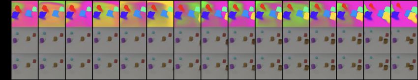
Under review as a conference paper at ICLR 2021

Figure 1: Unsupervised Video Decomposition. Our approach allows to infer precise segmentations
of the objects via interpretable latent representations, that can be used to decompose each frame and
simulate the future dynamics, all in unsupervised fashion. Whenever a new object emerges into a
frame the model dynamical adapts and uses one of the segmentation slots to assign to the new object.

In computer vision, it has been a long-held belief that motion carries important information for
segmenting objects (Jepson et al., 2002; Weiss & Adelson, 1996). Armed with this intuition, we
propose a spatio-temporal amortized inference model capable of not only unsupervised multi-object
scene decomposition, but also of learning and leveraging the implicit probabilistic dynamics of each
object from perspective raw video alone. This is achieved by introducing temporal dependencies
between the latent variables across time. As such, IODINE (Greff et al., 2019) could be considered a
special (spatial) case of our spatio-temporal formulation. Modeling temporal dependencies among
video frames also allows us to make use of conditional priors (Chung et al., 2015) for variational
inference, leading to more accurate and efficient inference results.
The resulting model, illustrated in Fig. 1, achieves superior performance on complex multi-object
benchmark datasets (Bouncing Balls and CLEVRER) with respect to state-of-the-art models, includ-
ing R-NEM (Van Steenkiste et al., 2018) and IODINE (Greff et al., 2019) in terms of segmentation,
prediction, and generalization. Our model has a number of appealing properties, including tempo-
ral extrapolation, computational efficiency, and the ability to work with complex data exhibiting
non-linear dynamics, colors, and changing number of objects within the same video sequence. In
addition, we introduce an entropy prior to improve our model’s performance in scenarios where
object appearance alone is not sufficiently distinctive (e.g., greyscale data).

2    R ELATED WORK
Unsupervised Scene Representation Learning. Unsupervised scene representation learning can
generally be divided into two groups: attention-based methods, which infer latent representations
for each object in a scene, and more complex and powerful iterative refinement models, which often
make use of spatial mixtures and can decompose a scene into a collection of estimated components by
grouping pixels together. Attention-based methods, such as AIR (Eslami et al., 2016) (Xu et al., 2019)
and SPAIR (Crawford & Pineau, 2019b), decompose scenes into latent variables representing the
appearance, position, and size of the underlying objects. However, both methods can only infer the
objects’ bounding boxes and have not been shown to work on non-trivial 3D scenes with perspective
distortions and occlusions. MoNet (Burgess et al., 2019) is the first model in this family tackling more
complex data and inferring representations that can be used for instance segmentation of objects. On
the other hand, it is not a probabilistic generative model and thus not suitable for density estimation.
GENESIS (Engelcke et al., 2020) extends it and alleviates some of its limitations by introducing
a probabilistic framework and allowing for spatial relations between the objects. DDPAE (Hsieh
et al., 2018) is a framework that uses structured probabilistic models to decompose a video into
low-dimensional temporal dynamics with the sole purpose of prediction. It is shown to operate on
binary scenes with no perspective distortion and is not capable of generating per-object segmentation
masks. Iterative refinement models started with Tagger (Greff et al., 2016) that reasons about the
segmentation of its inputs. However, it does not allow explicit latent representations and cannot be
scaled to more complex images. NEM (Greff et al., 2017), as an extension of Tagger, uses a spatial
mixture model inside an expectation maximization framework, but is limited to binary data. Finally,
IODINE (Greff et al., 2019) is a notable example of a model employing iterative amortized inference
w.r.t. a spatial mixture formulation and achieves state-of-the-art performance in scene decomposition
and segmentation.
Unsupervised Video Tracking and Object Detection. SQAIR (Kosiorek et al., 2018),
SILOT (Crawford & Pineau, 2019a) and SCALOR (Jiang et al., 2020) are temporal extensions

                                                   2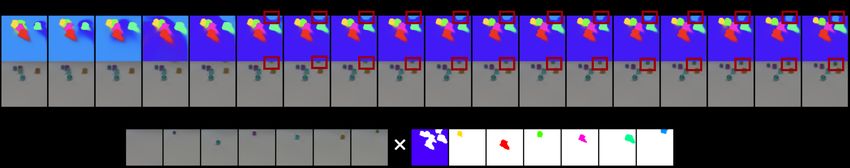
Under review as a conference paper at ICLR 2021

of the static attention-based models that are tailored to tracking and object detection tasks. SQAIR is
restricted to binary data and operates at the level of bounding boxes. SILOT and SCALOR are more
expressive and can cope with cluttered scenes, a larger numbers of objects, and dynamic backgrounds,
but do not work on colored perspective1 data; accurate segmentation remains a challenge.
Unsupervised Video Decomposition and Segmentation. Models employing spatial mixtures and
iterative inference in a temporal setting are closest to our method from a technical perspective. Notably,
there are only few models falling into this line of work: RTagger (Prémont-Schwarz et al., 2017) is a
recurrent extension of Tagger and has same limitations as its predecessor. R-NEM (Van Steenkiste
et al., 2018) effectively learns the objects’ dynamics and interactions through a relational module and
can produce segmentations but is limited to orthographic binary data.
Methods without Latent Modeling. GAN-based ReDO (Chen et al., 2019) uses a model built
around the assumption that object regions are independent, guiding the generator by drawing objects’
pixel regions separately and composing them after segmentation. Another model (Arandjelović &
Zisserman, 2019) employs the same principles but guide the generator by copying a region of an
image into another one. Both architectures are shown to operate on static images only and do not
have a clearly interpretable latent space or prediction capabilities.
Our method allows an effective use of temporal information in object-centric decompositions of
colored video data. This places our approach between methods like R-NEM, which strictly operates
on binary data, and IODINE, whose usage of temporal information is ad-hoc and produces results of
limited quality (Table 1). In practice, we leverage a 2D-LSTM and employ an implicit modeling of
dynamics by incorporating the hidden states into a conditional prior in the efficient runtime manner.

3       DYNAMIC V IDEO D ECOMPOSITION
We now introduce our dynamic model for unsupervised video decomposition. Our approach builds
upon a generative model of multi-object representations and leverages elements of iterative amortized
inference. We briefly review both concepts (§3.1) and then introduce our model (§3.2).

3.1       BACKGROUND
Multi-Object Representations. The multi-object framework introduced in Greff et al. (2019)
decomposes a static image x = (xi )i ∈ RD into K objects (including background). Each object
is represented by a latent vector z(k) ∈ RM capturing the object’s unique appearance and can be
thought of as an encoding of common visual properties, such as color, shape, position, and size.
For each z(k) independently, a broadcast decoder (Watters et al., 2019) generates pixelwise pairs
    (k)  (k)
(mi , µi ) describing the assignment probability and appearance of pixel i for object k. Together,
they induce the generative image formation model
                                              D X
                                                K
                                                          (k)         (k)
                                              Y
                                   p(x|z) =             mi N (xi ; µi , σ 2 ),                                 (1)
                                              i=1 k=1
                    PK       (k)
where z = (z(k) )k , k=1 mi = 1 and σ is the same and fixed for all i and k. The original image
                                                                          PK    (k) (k)
pixels can be reconstructed from this probabilistic representation as x
                                                                      ei = k=1 mi µi .
Iterative Amortized Inference. Our approach leverages the iterative amortized inference frame-
work (Marino et al., 2018), which uses the learning to learn principle (Andrychowicz et al., 2016) to
close the amortization gap (Cremer et al., 2017) typically observed in traditional variational inference.
The need for such an iterative process arises due to the multi-modality of Eq.(1), which results in
an order invariance and assignment ambiguity in the approximate posterior that standard variational
inference cannot overcome (Greff et al., 2019).
                                                                                                    (k)
The idea of amortized iterative inference is to start with randomly guessed parameters λ1 for the
                            (k)
approximate posterior qλ (z1 |x) and update this initial estimate through a series of R refinement
steps. Each refinement step r ∈ {1, . . . , R} first samples a latent representation from qλ to evaluate
    1
        Perspective videos are more complex as objects can occlude one another and change in size over time.

                                                         3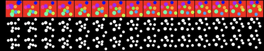
Under review as a conference paper at ICLR 2021

the ELBO L and then uses the approximate posterior gradients ∇λ L to compute an additive update
                                         (k)
fφ , producing a new parameter estimate λr+1 :
                            k                                        (k)      k                             (k)
                     z(k)
                      r   ∼ qλ (z(k)
                                 r |x),                                − λ(k)
                                                                  λr+1 ←  r + fφ (a
                                                                                   (k)
                                                                                       , hr−1 ),                                        (2)
                                        (k)
where a(k) is a function of zr , x, ∇λ L, and additional inputs (mirrors definition in Greff et al.
(2019)). The function fφ consists of a sequence of convolutional layers and an LSTM. The memory
                                    (k)
unit takes as input a hidden state hr−1 from the previous refinement step.

3.2    S PATIO -T EMPORAL I TERATIVE I NFERENCE
Our proposed model builds upon the concepts introduced in the previous section and enables robust
learning of dynamic scenes through spatio-temporal iterative inference. Specifically, we consider
                                                                                              (k)
the task of decomposing a video sequence x = (xt )Tt=1 = (xt,i )T,D
                                                                t,i=1 into K slot sequences (mt )t
                                           (k)
and K appearance sequences (µt )t . To this end, we introduce explicit temporal dependencies into
the sequence of posterior refinements and show how to leverage this contextual information during
decoding with a generative model. The resulting computation graph can be thought of as a 2D grid
with time dimension t and refinement dimension r (Fig. 2a). Propagation of information along these
two axes is achieved with a 2D-LSTM (Graves et al., 2007) (Fig. 2b), which allows us to model the
joint probability over the entire video sequence inside the iterative amortized inference framework.
The proposed method is expressive enough to model the multimodality of our image formation
process and posterior, yet its runtime complexity is smaller than that of its static counterpart.

3.2.1 VARIATIONAL O BJECTIVE
Since exact likelihood training is intractable, we formulate our task in terms of a variational objective.
In contrast to traditional optimization of the evidence lower bound (ELBO) through static encodings
of the approximate posterior, we incorporate information from two dynamic axes: (1) variational
estimates from previous refinement steps; (2) temporal information from previous frames. Together,
they form the basis for spatio-temporal variational inference via iterative refinements. Specifically,
we train our model by maximizing the following ELBO objective2 :
                                   PT     PRb h                                                                                    i
  LELBO (x) = Eqλ (z≤T ,R |x≤T )    t=1       r=1   β log (p (xt |x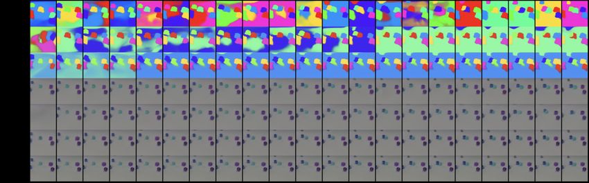
Under review as a conference paper at ICLR 2021

                            (a)                                                        (b)
Figure 2: Model Overview. (a) Inference in our model passes through a 2D grid in which light gray
cell (r, t) represents the r-th refinement at time t, dark gray cells are where the final reconstruction
is computed and no refinement is needed . Each light gray cell receives three inputs: a refinement
hidden state ht,r−1 , a temporal hidden state ht−1,Rb , and posterior parameters λt,r . The outputs are a
new hidden state ht,r and new posterior parameters λt,r+1 . (b) An example of the internal structure
of the highlighted cell from Fig. (a). We process the inputs with the help of a spatial broadcast
decoder and a 2D LSTM. The rest of the light gray cells have the same structure.

Note that the hidden state from the previous time step is always ht−1,Rb , i.e., the one computed during
                     b at time t − 1. Our reasoning for this is that the approximation of the posterior
the final refinement R
only improves with the number of refinements (Marino et al., 2018).
Temporal Conditioning. Inside the learning objective we set the prior and the likelihood to be
conditioned on the previous frames and the refinement steps. This naturally comes from an idea that
each frame is dependent on the predecessor’s dynamics and therefore latent representations should
follow the same property. Conditioning on the refinement steps is essential to the iterative amortized
inference procedure. To model the prior and the likelihood distributions accordingly we adopt the
approach proposed in Chung et al. (2015) but tailor it to our iterative amortized inference setting.
Specifically, the parameters of our Gaussian prior are now computed from the temporal hidden state
ht−1,Rb :
                     p(zt |x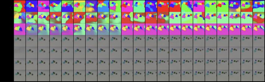
Under review as a conference paper at ICLR 2021

time t. According to Eq.(4), each such cell takes as input the hidden state from a previous refinement
ht,r−1 , the temporal hidden state ht−1,Rb , and the posterior parameters λt,r . Outputs of each light
gray cell are new posterior parameters λt,r+1 and a new hidden state ht,r . At the last refinement R
                                                                                                   b at
time t, the value of the refinement hidden state ht,r is assigned to a new temporal hidden state ht,Rb .
Training Objective. Instead of a direct optimization of Eq.(3), we propose two modifications that
we found to improve our model’s practical performance: (1) similar to observations made by (Greff
et al., 2019), we found that color is an important factor for high-quality segmentations. In the absence
                                                                                                     (k)
of such information, we mitigate the arising ambiguity by maximizing the entropy of the masks mt,r,i
along the slot dimension k, i.e., we train our model by maximizing the objective
                                                 D X
                                                   K
                                                               (k)         (k)
                                                 X
                                     LELBO + γ               mt,r,i log(mt,r,i ),                       (7)
                                                  i=1 k=1

where γ defines the weight of the entropy loss. (2) In addition to the entropy loss, we also prioritize
later refinement steps by weighting the terms in the inner sum of Eq.(3) with Rrb .
Prediction. On top of pure video decomposition, our model is also able to simulate future frames
xT +1 , . . . , xT +T 0 . Because our model requires image data xt as input, which is not available during
simulation of new frames, we use the reconstructed image x    et in place of xt to compute the likelihood
p(xt |x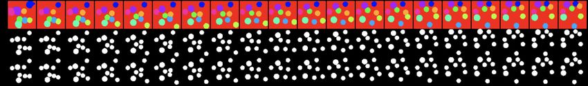
Under review as a conference paper at ICLR 2021

Table 1: Quantitative Evaluation (Scene Decomposition). We show our model’s ability to produce
high-quality instance segmentations for sequences with varying length. We test on sequences with 4
balls and two different types of data (binary, colored) for Bouncing Balls and on sequences with 3-5
objects for CLEVRER. Note, R-NEM does not cope with color data; hence we only run it on binary.

                                                          Bouncing Balls
                                      ARI (↑)                              F-ARI (↑)                        MSE (↓)
          Length         10      20         30     40         10        20        30     40       10      20      30      40
          R-NEM        0.5031   0.6199 0.6632    0.6833     0.6259     0.7325 0.7708   0.7899   0.0252   0.0138 0.0096   0.0076
 binary

          IODINE                     0.0318                                 0.9986                           0.0018
          SEQ-IODINE   0.0230   0.0223 0.0021    -0.0201    0.8645     0.6028 0.5444   0.4063   0.0385   0.0782 0.0846   0.0968
          Our          0.7169   0.7263 0.7286     0.7294    0.9999     0.9999 0.9999   0.9999   0.0004   0.0004 0.0004   0.0004
          IODINE                     0.5841                                 0.9752                           0.0014
 color

          SEQ-IODINE   0.3789   0.3743 0.3225    0.2654     0.7517     0.8159 0.7537   0.6734   0.0160   0.0164 0.0217   0.0270
          Our          0.7275   0.7291 0.7298    0.7301     1.0000     1.0000 0.9999   0.9999   0.0002   0.0002 0.0002   0.0002
                                                           CLEVRER
                                   ARI (↑)                                 F-ARI (↑)                        MSE (↓)
          Length        10       20         30     40         10        20        30    40       10       20      30      40
          IODINE                    0.1791                                 0.9316                            0.0004
 color

          SEQ-IODINE   0.1171   0.1378 0.1558    0.1684     0.8520     0.8774 0.8780   0.8759   0.0009   0.0009 0.0010   0.0010
          Our          0.2220   0.2403 0.2555    0.2681     0.9182     0.9258 0.9309   0.9312   0.0003   0.0003 0.0003   0.0003

framework. However, as noted in Greff et al. (2019), it can be readily applied to temporal sequences
by feeding a new video frame to each iteration of the LSTM in the refinement network. We call this
variant SEQ-IODINE. Since we can perform simulation of short sequences, we include a comparison
of the predictive power of our model against DDPAE (Hsieh et al., 2018).

4.2 E VALUATION M ETRICS
ARI. The Adjusted Rand Index (Rand, 1971; Hubert & Arabie, 1985) is a measure of clustering
similarity. It is computed by counting all pairs of samples that are assigned to the same or different
clusters in the predicted and true clusterings. It ranges from -1 to 1, with score of 0 indicating
a random clustering and 1 indicating a perfect match. We treat each pixel as one sample and its
segmentation as the cluster assignment.
F-ARI. The Foreground Adjusted Rand Index is a modification of the ARI score ignoring background
pixels, which often occupy the majority of the image. We argue that both metrics are necessary to
assess the segmentation quality of a video decomposition method; this metric is also used in (Greff
et al., 2019; Van Steenkiste et al., 2018).
MSE. The mean squared error between pixels of the reconstructed x
                                                                b and the ground truth frames x.

4.3 V IDEO D ECOMPOSITION
We evaluate the models on a video decomposition task at different sequence lengths. As shown in
Table 1, our model outperforms the baselines regardless of the presence of color information, which
further reduces the error. Our model performs at least 7% better than R-NEM on all metrics and
at least 20% than IODINE on ARI and MSE. Since R-NEM cannot cope well with colored data
or the perspective of scenes, it is only evaluated on the Bouncing Balls dataset (binary), producing
high-error results in the first frames, a phenomenon not observed with our model. IODINE is not
designed to utilize temporal information. On both datasets, IODINE’s results are therefore computed
independently on each frame of the longest sequence. By processing frames separately, IODINE does
not keep the same object-slot assignment, which we ignore when computing the scores. SEQ-IODINE
tends to perform even worse than IODINE in many experiments, which we attributed to exploding
gradients caused by limited refinement steps and a lack of dynamics modeling.

4.4 G ENERALIZATION
We investigated how well our model adapts to a higher number of objects, evaluating its performance
on the Bouncing Balls dataset (6 to 8 objects) and on the CLEVRER dataset (6 objects). Table 2
shows that our F-ARI and MSE scores are at least 50% better than those for R-NEM, and ARI scores
are just marginally worse and only on the binary data. In comparison to IODINE we are at least
4% better across all metrics. For the Bouncing Balls dataset we have also investigated the impact of

                                                                   7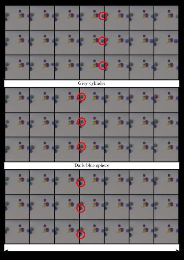
Under review as a conference paper at ICLR 2021

Figure 3: Qualitative Evaluation (Bouncing Balls). Our model can generalize to sequences with 8
balls when trained on 4 balls. Top-to-bottom: output masks, reconstructions, and ground truth video.
                               Bouncing Balls                                     Bouncing Balls                                               CLEVRER
                     1.0                          OUR
                                                  DDPAE                                        ARI Our                                                      ARI
                                                                                               ARI Our (color)                                              F-ARI
                                                                                               ARI R-NEM
                                                                                                                               1.0
 Cosine similarity

                     0.9                                                                       F-ARI Our
                                                                                               F-ARI Our (color)
                                                                        1.0                    F-ARI R-NEM
                                                                                                                               0.8

                                                            ARI/F-ARI

                                                                                                                   ARI/F-ARI
                     0.8                                                0.9
                                                                                                                               0.6
                                                                        0.8
                     0.7                                                                                                       0.4
                                                                        0.7

                                                                        0.6                                                    0.2
                     0.6
                           1    2     3     4        5
                               Simulation steps                               3     5      7
                                                                                  Simulation steps
                                                                                                            10                       3     5       7
                                                                                                                                         Simulation steps
                                                                                                                                                             10

Figure 4:       Velocity predic-
                                                          Figure 5: Prediction. We show the (F-)ARI for 3, 5, 7, and 10 simulated
tions.Cosine similarity for 5
                                                          frames after 20 inference steps.
simulated frames after 10 inference
steps.

changing the total number of possible colors to 4 and 8. The former resulting in duplicate colors for
different objects and the latter in unique colors for each object. The higher MSE scores for the 8 balls
variant is due to the model not being able to reconstruct the unseen colors. Sample qualitative results
are shown in Fig. 3 and 6, while more can be found in Appendix F.

4.5 P REDICTION
We compare the predictions of our model (Section 3.2.3) to those of R-NEM after 20 steps of
inference on 10 predicted steps on the Bouncing Balls dataset (Fig. 5 left). As we can see from the
results our model is superior to R-NEM on a shorter sequences, however for the longer sequences
we are outperforming R-NEM only on colored data. Our model is capable of more accurate frame
prediction than R-NEM on the Bouncing Balls dataset during the first few predicted frames (5-7),
with predictions slowly diverging over time due to the temporal consistency. This behavior is also
observable on the CLEVRER dataset (Fig. 5 right), albeit to a lesser extent, likely because the objects
dynamics are less, even if non-linear. In Figure 4 we compute velocity vectors between bounding
box centroids and compare the cosine similarity to the predictions of DDPAE on the Bouncing balls
dataset. As expected, our model outperforms DDPAE on the first three frames and then declines in
quality. This behavior is not surprising and in line with the results reported in Fig.5
4.6 A BLATION
The quantitative results of an ablation study on the binary Bouncing Balls dataset and CLEVRER are
shown in Table 3. We investigate the effects of the efficient grid, conditional prior and generation,
length of training sequences and entropy term on the performance of our model; all contributions are
necessary and important. Note that the base models are too large to be trained on 40 frames, which
confirms the superiority of our model in terms of both runtime and memory. The CLEVRER dataset
is not binary, which is why we do not include the entropy term (see Section 3.2.3). We validate our
choice of Rb and compare it to alternative options in a supplemental study discussed in Appendix F.2.

5                    C ONCLUSION AND D ISCUSSION
We presented a novel unsupervised learning framework capable of precise scene decomposition in
multi-object videos with complex appearance and motion. Our temporal component enables modeling
of dynamics inside the amortized iterative inference framework but also improves the quality of the
results overall. From our quantitative and qualitative comparisons with IODINE and SEQ-IODINE,
we see that our model shows more accurate results on the decomposition task. We can detect new

                                                                                   8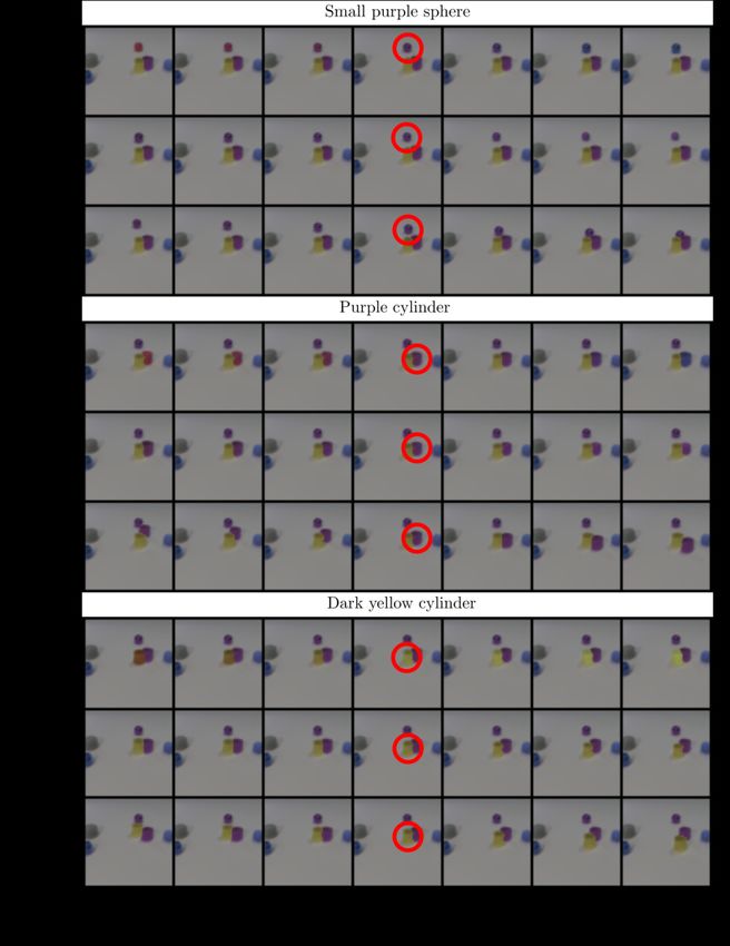
Under review as a conference paper at ICLR 2021
Table 2: Generalization. At test time, we change Table 3: Ablation Study. A 2D-LSTM extension of
the number of slots in the models from 5 to 9 IODINE trained on sequences of 20 frames is unstable and
for the Bouncing Balls test dataset (6-8 balls), its output segmentation lacks precision and consistency. Our
and from 6 to 7 for the CLEVRER test dataset (6 efficient version of 2D-LSTM grid (Fig. 2a) and the condi-
objects). tional prior and generation increase both segmentation and
reconstruction quality. By training these models on longer
Bouncing Balls sequences of 40 frames we observe further improvements.
ARI (↑) F-ARI (↑) MSE (↓)
Le py
th
+G
tro
0.4484
ng
R-NEM 0.6377 0.0328
se
rid
CP
Ba
En
ARI (↑) F-ARI (↑) MSE (↓)
binary
G
IODINE 0.0271 0.9969 0.0040
SEQ-IODINE 0.0263 0.8874 0.0521 X 20 0.0126 0.7765 0.0340
Our 0.4453 0.9999 0.0008 X X X 20 0.2994 0.9999 0.0010
BB
IODINE (4) 0.4136 0.8211 0.0138 X X X 40 0.3528 0.9998 0.0010
IODINE (8) 0.2823 0.7197 0.0281 X X X X 40 0.7263 0.9999 0.0004
color
SEQ-IODINE (4) 0.2068 0.5854 0.0338 X 20 0.1900 0.8200 0.0011
CLEVRER
SEQ-IODINE (8) 0.1571 0.5231 0.0433 X X 20 0.1100 0.9000 0.0005
Our (4) 0.4275 0.9998 0.0004 X X X 20 0.2403 0.9258 0.0003
Our (8) 0.4317 0.9900 0.0114 X X 40 0.1700 0.9100 0.0005
X X X 40 0.2681 0.9312 0.0003
CLEVRER [Base: base model using 2D-LSTM; Grid: efficient
ARI (↑) F-ARI (↑) MSE (↓) triangular grid structure (Fig. 2a); CP+G: conditional prior
IODINE 0.2205 0.9305 0.0006 and generation; Length: sequence length; Entropy: entropy
color
SEQ-IODINE 0.1482 0.8645 0.0012 term (Eq.(7)]
Our 0.2839 0.9355 0.0004
Figure 6: Qualitative Evaluation (CLEVRER). Our model can generalize to sequences with 6 objects. We
also demonstrate the ability to handle a dynamically changing number of objects, ranging from 4 in the beginning
to 6 at the end.
objects faster and are less sensitive to color, because our model can leverage the objects’ motion cues.
For our experiments, we have chosen a setup consistent with other SOTA methods and a focus on
the objects’ dynamics. Our model is currently not targeting complex textured datasets, as they are
not designed for unsupervised learning and impose additional challenges, such as limited coverage
of the input space as well as a superposition of the scene’s intrinsic components (object location,
articulation, motion, albedo, shading, etc.). We show and discuss the segmentation of a real-world
video stream in Fig. 7. Self-supervised methods for video segmentation, which attempt to learn
image representations through features, motion or specific tasks, are an alternative but not capable of
inferring disentangled representations or extracting interpretable features (e.g. appearance, color).
They are typically also not robust to object occlusions, object (dis)appearances, and object ordering
(Fig. 14). We refer to Appendix E for an extended discussion and future work.
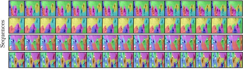
Figure 7: Qualitative evaluation on real-world data. Qualitative Evaluation (Grand Central Station). We can
observe that our method is very consistent in separating the image regions belonging to different objects as they
move in the scene. This dataset is particularly challenging for its background texture, complex lighting and
shadows. Please zoom in to allow better clarity.
9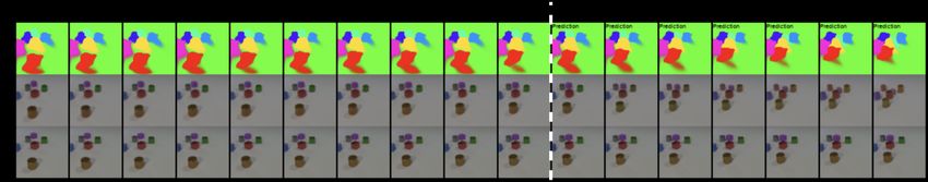
Under review as a conference paper at ICLR 2021

R EFERENCES
M. Andrychowicz, M. Denil, S. Gomez, M. W. Hoffman, D. Pfau, T. Schaul, and N. de Freitas.
 Learning to learn by gradient descent by gradient descent. In NIPS, 2016.
Relja Arandjelović and Andrew Zisserman. Object discovery with a copy-pasting gan. arXiv preprint
  arXiv:1905.11369, 2019.
Christopher P Burgess, Loic Matthey, Nicholas Watters, Rishabh Kabra, Irina Higgins, Matt Botvinick,
  and Alexander Lerchner. Monet: Unsupervised scene decomposition and representation. arXiv
  preprint arXiv:1901.11390, 2019.
Mickaël Chen, Thierry Artières, and Ludovic Denoyer. Unsupervised object segmentation by
 redrawing. In Advances in Neural Information Processing Systems, pp. 12726–12737, 2019.
Kyunghyun Cho, Bart Van Merriënboer, Caglar Gulcehre, Dzmitry Bahdanau, Fethi Bougares, Holger
  Schwenk, and Yoshua Bengio. Learning phrase representations using rnn encoder-decoder for
  statistical machine translation. In EMNLP, 2014.
Junyoung Chung, Kyle Kastner, Laurent Dinh, Kratarth Goel, Aaron C Courville, and Yoshua Bengio.
  A recurrent latent variable model for sequential data. In NIPS, pp. 2980–2988, 2015.
Junyoung Chung, Sungjin Ahn, and Yoshua Bengio. Hierarchical multiscale recurrent neural networks.
  In ICLR, 2017.
Eric Crawford and Joelle Pineau. Exploiting spatial invariance for scalable unsupervised object
  tracking. In AAAI, 2019a.
Eric Crawford and Joelle Pineau. Spatially invariant unsupervised object detection with convolutional
  neural networks. In AAAI, pp. 3412–3420, 2019b.
C. Cremer, X. Li, and D. Duvenaud. Inference suboptimality in variational autoencoders. In NIPS
  Workshop on Advances in Approximate Bayesian Inference, 2017.
Martin Engelcke, Adam R Kosiorek, Oiwi Parker Jones, and Ingmar Posner. Genesis: Generative
 scene inference and sampling with object-centric latent representations. In ICLR, 2020.
SM Ali Eslami, Nicolas Heess, Theophane Weber, Yuval Tassa, David Szepesvari, Geoffrey E
 Hinton, et al. Attend, infer, repeat: Fast scene understanding with generative models. In NIPS, pp.
 3225–3233, 2016.
Alex Graves, Santiago Fernández, and Jürgen Schmidhuber. Bidirectional lstm networks for improved
  phoneme classification and recognition. In Włodzisław Duch, Janusz Kacprzyk, Erkki Oja, and
  Sławomir Zadrożny (eds.), Artificial Neural Networks: Formal Models and Their Applications –
  ICANN 2005, pp. 799–804, Berlin, Heidelberg, 2005. Springer Berlin Heidelberg. ISBN 978-3-
  540-28756-8.
Alex Graves, Santiago Fernández, and Jürgen Schmidhuber. Multi-dimensional recurrent neural
  networks. In International conference on artificial neural networks, pp. 549–558. Springer, 2007.
Klaus Greff, Antti Rasmus, Mathias Berglund, Tele Hao, Harri Valpola, and Jürgen Schmidhuber.
  Tagger: Deep unsupervised perceptual grouping. In NIPS, pp. 4484–4492, 2016.
Klaus Greff, Sjoerd Van Steenkiste, and Jürgen Schmidhuber. Neural expectation maximization. In
  NIPS, pp. 6691–6701, 2017.
Klaus Greff, Raphaël Lopez Kaufmann, Rishab Kabra, Nick Watters, Chris Burgess, Daniel Zoran,
  Loic Matthey, Matthew Botvinick, and Alexander Lerchner. Multi-object representation learning
  with iterative variational inference. arXiv preprint arXiv:1903.00450, 2019.
Irina Higgins, Loic Matthey, Arka Pal, Christopher Burgess, Xavier Glorot, Matthew Botvinick,
   Shakir Mohamed, and Alexander Lerchner. beta-vae: Learning basic visual concepts with a
   constrained variational framework. In ICLR, 2017.

                                                 10
Under review as a conference paper at ICLR 2021
G.E. Hinton and T.J. Sejnowski. Learning and relearning in boltzmann machines. Parallel Distributed
Processing: Explorations in the Microstructure of Cognition, 1:282–317, 1986.
Sepp Hochreiter and Jürgen Schmidhuber. Long short-term memory. Neural computation, 9(8):
1735–1780, 1997.
Jun-Ting Hsieh, Bingbin Liu, De-An Huang, Li Fei-Fei, and Juan Carlos Niebles. Learning to
decompose and disentangle representations for video prediction. CoRR, abs/1806.04166, 2018.
URL http://arxiv.org/abs/1806.04166.
Lawrence Hubert and Phipps Arabie. Comparing partitions. Journal of classification, 2(1):193–218,
1985.
A. Jepson, D. Fleet, and M. Black. A layered motion representation with occlusion and compact
spatial support. In ECCV, pp. 692–706, 2002.
Jindong Jiang, Sepehr Janghorbani, Gerard De Melo, and Sungjin Ahn. Scalor: Generative world
models with scalable object representations. In ICLR, 2020.
Diederik P Kingma and Jimmy Ba. Adam: A method for stochastic optimization. arXiv preprint
arXiv:1412.6980, 2014.
Diederik P. Kingma and Max Welling. Auto-encoding variational bayes. In ICLR, 2014.
Adam Kosiorek, Hyunjik Kim, Yee Whye Teh, and Ingmar Posner. Sequential attend, infer, repeat:
Generative modelling of moving objects. In NeurIPS, pp. 8606–8616, 2018.
Jiasen Lu, Dhruv Batra, Devi Parikh, and Stefan Lee. Vilbert: Pretraining task-agnostic visiolinguistic
representations for vision-and-language tasks. In NeurIPS, 2019.
Joseph Marino, Yisong Yue, and Stephan Mandt. Iterative amortized inference. In ICML, 2018.
D. Marr. A theory for cerebral neocortex. Proceedings of the Royal Society of London, Series B(176):
161–234, 1970.
M. Noroozi and P. Favaro. Unsupervised learning of visual representations by solving jigsaw puzzles.
In ECCV, 2016.
D. Pathak, P. Krahenbuhl, J. Donahue, T. Darrell, and A. A. Efros. Context encoders: Feature learning
by inpainting. In CVPR, 2016.
Isabeau Prémont-Schwarz, Alexander Ilin, Tele Hao, Antti Rasmus, Rinu Boney, and Harri Valpola.
Recurrent ladder networks. In NIPS, pp. 6009–6019, 2017.
William M Rand. Objective criteria for the evaluation of clustering methods. Journal of the American
Statistical association, 66(336):846–850, 1971.
Adam Santoro, David Raposo, David G Barrett, Mateusz Malinowski, Razvan Pascanu, Peter
Battaglia, and Timothy Lillicrap. A simple neural network module for relational reasoning. In
NIPS, pp. 4967–4976, 2017.
Chen Sun, Austin Myers, Carl Vondrick, Kevin Murphy, and Cordelia Schmidt. Videobert: A joint
model for video and language representation learning. In ICCV, 2019.
Hao Tan and Mohit Bansal. Lxmert: Learning cross-modality encoder representations from trans-
formers. In Conference on Empirical Methods in Natural Language Processing, 2019.
Sjoerd Van Steenkiste, Michael Chang, Klaus Greff, and Jürgen Schmidhuber. Relational neural
expectation maximization: Unsupervised discovery of objects and their interactions. In ICLR,
2018.
Ashish Vaswani, Noam Shazeer, Niki Parmar, Jakob Uszkoreit, Llion Jones, Aidan N Gomez, Łukasz
Kaiser, and Illia Polosukhin. Attention is all you need. In NIPS, pp. 5998–6008, 2017.
11Under review as a conference paper at ICLR 2021
P. Vincent, H. Larochelle, Y. Bengio, and P. A. Manzagol. Extracting and composing robust features
with denoising autoencoders. In ICML, 2008.
C. Vondrick, H. Pirsiavash, and A. Torralba. Anticipating visual representations with unlabeled
videos. In CVPR, 2016.
Nicholas Watters, Loic Matthey, Christopher P Burgess, and Alexander Lerchner. Spatial broadcast
decoder: A simple architecture for learning disentangled representations in vaes. arXiv preprint
arXiv:1901.07017, 2019.
Y. Weiss and E. Adelson. A unified mixture framework for mo- tion segmentation: Incorporating
spatial coherence and estimating the number of models. In CVPR, pp. 321–326, 1996.
Kun Xu, Chongxuan Li, Jun Zhu, and Bo Zhang. Multi-objects generation with amortized struc-
tural regularization. CoRR, abs/1906.03923, 2019. URL http://arxiv.org/abs/1906.
03923.
Kexin Yi, Chuang Gan, Yunzhu Li, Pushmeet Kohli, Jiajun Wu, Antonio Torralba, and Joshua B
Tenenbaum. Clevrer: Collision events for video representation and reasoning. In ICLR, 2020.
R. Zhang, P. Isola, and A. A. Efros. Colorful image colorization. In ECCV, 2016.
B. Zhou, X. Wang, and X. Tang. Understanding collective crowd behaviors: Learning a mixture
model of dynamic pedestrian-agents. In 2012 IEEE Conference on Computer Vision and Pattern
Recognition, pp. 2871–2878, 2012. doi: 10.1109/CVPR.2012.6248013.
A BASELINES
A.1 R-NEM
We use the R-NEM (Van Steenkiste et al., 2018) authors’ original implementation and their publicly
available models: https://github.com/sjoerdvansteenkiste/Relational-NEM.
A.2 IODINE
Our IODINE experiments are based on the following PyTorch implementation: https://github.
com/MichaelKevinKelly/IODINE. We use the same parameters as in this code, with the
exceptions of β = 10 (weight factor) and, for the Bouncing Balls experiments, R = 6 (refinement
steps). The majority of the hyperparameters shared between our own model and IODINE are identical.
A.3 SEQ-IODINE
In order to test the sequential version of IODINE, we use the regularly trained IODINE model but
change the number of refinement steps to the number of video frames during testing. During each
refinement step, instead of computing the error between the reconstructed image and the ground truth
image, we use the next video frame. Since the IODINE model was trained on R = 6 refinement steps,
extending the number of refinement steps to the video length leads to exploding gradients. This effect
is especially problematic in the binary Bouncing Balls dataset with 20, 30 and 40 frames per video,
because the scores of the static model are already low. We deal with this issue by clamping with max
= 10 and min = −10 the gradients and the δ refinement value in this experiment6 . SEQ-IODINE’s
weak performance, especially w.r.t. the ARI, reflect the gradual divergence from the optimum as the
number of frames increases.
B DATASETS
Bouncing Balls. Bouncing Balls is a dataset provided by the authors of R-NEM (Van Steenkiste
et al., 2018).Dataset contains balls with different masses corresponding to their radii. The balls are
6
Please note that clamping was done only when applied to binary Bouncing Balls for 20, 30 and 40 frames.
12Under review as a conference paper at ICLR 2021
initialized with random initial positions, masses and velocities. Balls bounce elastically against each
other(without occlusions) and the image window. We use the train and test splits of this dataset in
two different versions: binary and color. For the color version, we randomly choose 4 colors for the
4-balls (sub-)dataset. For the 6-8 balls test data, we color them in 2 different ways: 4 colors (same
as train) and 8 colors (4 from train, 4 new ones). Note that the former results in identical colors for
multiple objects, while the latter guarantees unique colors for each object.
CLEVRER. Each video in the CLEVRER dataset contains at least one collision and (dis)appearence
event making occlusions possible and frequent. Objects’ initial velocities are approximately
±2.5 m/s2 . Each object has one of eight distinct colors and one of 38 two materials (metal or
rubber). In addition, two objects can have the same color but different material.
The version of the CLEVRER dataset (Yi et al., 2020) used in this work was processed as follows:
• Train split, validation split and validation annotations were obtained from the official website:
http://clevrer.csail.mit.edu/. We use the validation set as test set, because
the test set does not contain annotations.
• For training, we use the original train split. Our minimal preprocessing consists of cropping
the frames along the width axis by 40 pixels on both sides, followed by a uniform downscal-
ing to 64x64 pixels. Since the length of each video is 128 frames and the maximum number
of frames during training was 40, we split the videos into multiple sequences to obtain a
larger number of training samples.
• For testing, we trim the videos to a subsequence containing at least 3 ob-
jects and object motion. We compute these subsequences by running the script
(slice_videos_from_annotations.py in the attached code) from the folder with the validation
split and validation annotations.
• The test set ground truth masks can be downloaded from here. The masks and the prepro-
cessed test videos will be grouped into separate folders based on the number of objects in a
video.
C H YPERPARAMETERS
Initialization. We initialize the parameters of the posterior λ by sampling from U(−0.5, 0.5). In
all experiments, we use a latent dimensionality dim(z) = 64, such that dim(λ) = 128. Horizontal
and vertical hidden states and cell states are of size 128, initialized with zeros. qλ is the posterior
probability per slot of the likelihood p(x|z), which is a Gaussian mixture model. The variance of the
likelihood is set to σ = 0.3 in all experiments.
Experiments on Bouncing Balls. For this experiment, we have explored several values of R
(refinement steps) and empirically found R = 6 to be optimal in terms of accuracy and efficiency.
Refining the posterior more than 6 times does not lead to any substantial improvement, however, the
time and memory consumption is significantly increased. For the 4-balls dataset, we use K = 5 slots
for train and test. For our tests on 6-8 balls, we use K = 9 slots. This protocol is identical to the one
used in R-NEM (Van Steenkiste et al., 2018). Furthermore, we set β = 100.0 and scale the KL term
by ψ = 10. The weight of the entropy term is set to γ = 0.1 in the binary case. As expected, the
effect of the entropy term is most pronounced with binary data, so we set γ = 0 in all experiments
with RGB data.
Experiments on CLEVRER. We keep the default number of iterative refinements at R = 5, because
we did not observe any substantial improvements from a further increase. We use K = 6 slots during
training, K = 6 slot when testing on 3-5 objects and K = 7 slots when testing on 6 objects.
D T RAINING
We use ADAM (Kingma & Ba, 2014) for all experiments, with a learning rate of 0.0003 and default
values for all remaining parameters. During training, we gradually increase the number of frames
per video, as we have found this to make the optimisation more stable. We start with sequences of
length 4 and train the model until we observe a stagnant loss or posterior collapse. At the beginning
13Under review as a conference paper at ICLR 2021
of training, the batch size is 32 and is gradually decreased negatively proportional to the number of
frames in the video.
D.1 I NFRASTRUCTURE AND RUNTIME
We train our models on 8 GeForce GTX 1080 Ti GPUs, which takes approximately one day per
model.
D.2 C ODE
We have attached the code and the pretrained models to reproduce the experimental results. Please
see README file in the code folder to help you with running.
E D ISCUSSION AND F UTURE WORK
Introduction of a temporal component not only enables modelling of dynamics inside the amortized
iterative inference framework but also improves the quality of the results overall. From our quantitative
and qualitative comparisons with IODINE and SEQ-IODINE, we see that our model shows more
accurate results on the decomposition task. We can detect new objects faster and are less sensitive to
color, because our model can leverage the objects’ motion cues. The ability to work with complex
colored data, a property inherited from IODINE, means that we significantly outperform R-NEM.
However, R-NEM is a stronger model when it comes to prediction of longer sequences, owing
to its ability to model the relations between the objects in the scene. Similar ideas were used
in SQAIR (Kosiorek et al., 2018) and GENESIS (Engelcke et al., 2020) by adding a relational
RNN (Santoro et al., 2017). Integration of these concepts into our framework is a promising direction
for future research. Another possible route is an application of our model to complex real-world
scenarios. However, given that such datasets typically contain a much higher number of objects, as
well as intricate interactions and spatially varying materials, we consider the resulting scalability
questions as a separate line of research.
F A DDITIONAL E XPERIMENTS
F.1 P REDICTION
3.0 1e 2
Bouncing Balls 1.2 1e 3
CLEVRER
Our Our
Our (color) 1.1
2.5 R-NEM
1.0
2.0 0.9
MSE
MSE
1.5 0.8
0.7
1.0
0.6
0.5 0.5
0.4
3 5 7 10 3 5 7 10
Simulation steps Simulation steps
Figure 8: Mean Squared Error for the prediction experiment. We have computed MSE for the same
experimental set up as on Fig. 5. As expected the MSE increases with number of simulation steps.
Similarly to ARI and F-ARI scores our model outperforms R-NEM on a first steps of simulation,
however the error function of our model is grows faster comparatively to R-NEM and we sooner
diverge from the accurate simulation.
14Under review as a conference paper at ICLR 2021
F.2 A BLATIONS
The performance of our model is governed by the function R b = max(R − t, 1), where R is the
free parameter. In Table 4 we explore values of R ranging from 2 to 10. We see performance
saturation at R ≈ 4. We also explore an alternative choice R
balt. (Table 5), which shows decreased
performance compared to R. b The number of slots K could be determined via cross-validation, but
for comparability to other SOTA methods we assume it to be given.
Table 4: Performance as a Function of Parameter R.
ARI (↑) F-ARI (↑) MSE (↓)(×10−4 )
R 2 4 8 10 2 4 8 10 2 4 8 10
BB bin. 0.34 0.71 0.73 0.73 0.93 0.99 0.99 0.99 424 6 5 8
BB col. 0.48 0.72 0.73 0.73 0.93 0.99 1.0 1.0 148 3 3 4
CLEVRER 0.21 0.24 0.23 0.22 0.84 0.92 0.93 0.94 11 3 3 3
Table 5: Ablation on the Form of the Function R.
b Rbalt. = R, when t = 0, and R
balt. = 1,
when t > 0.
ARI (↑) F-ARI (↑) MSE (↓)(×10−4 )
R
b R
balt R
b R
balt R
b R
balt
BB bin. 0.73 0.43 1.0 0.95 4 33.2
BB col. 0.73 0.57 1.0 0.97 2 11.9
CLEVRER 0.24 0.21 0.93 0.88 3 9
F.3 A DDITIONAL QUALITATIVE RESULTS
Figure 9: Video decomposition using our model applied on Bouncing Balls dataset with 4 balls.
Figure 10: Video decomposition using our model applied on Bouncing Balls dataset with 6-8 balls.
15Under review as a conference paper at ICLR 2021
Figure 11: Prediction on Bouncing Balls (colored) dataset.
Figure 12: Prediction on CLEVRER dataset.
(a)
(b)
Figure 13: Qualitative results for Ours vs. IODINE vs. SEQ-IODINE decomposition experiment.
(a) From the figure it is clear that our model can much sooner detect new objects emerging to the
frame, while SEQ-IODINE struggles to properly reconstruct and decompose them. And IODINE
doesn’t have any temporal consistence and reshuffles the slot order. (b). Here we can see that our
model is much more stable with time and it does not fail to detect objects, unlike IODINE and
SEQ-IODINE.
16Under review as a conference paper at ICLR 2021
(a) (b)
Figure 14: Disentanglement of the latent representations corresponding to distinct interpretable
features. CLEVRER latent walks along three different dimensions: color, size and position. We
chose a random frame and for each object’s representation in the scene dimensions were traversed
independently.
F.4 D ISENTANGLEMENT
We demonstrate that introducing a new temporal hidden state and an additional MLP in front of the
spatial broadcast decoder has not impacted its ability to separate each object’s representations and
disentangles them based on color, position, size and other features, similar to results shown in Greff
et al. (2019).
F.5 A NIMATIONS
Attached animations include the following files:
• bb_binary_4_balls.gif Animation of the segmentations of 4 binary Bouncing Balls. 50
frames. Here and everywhere else, unless explicitly specified, we also included full scene
decomposition and each object’s individual reconstruction.
• bb_binary_6_8_balls.gif Animation of the ability to generalize to 6-8 binary Bouncing
Balls. 40 frames.
• bb_colored_4_balls.gif Animation of the 4 colored Bouncing Balls. 50 frames.
• bb_colored_6_8_balls.gif Animation of the ability to generalize to 6-8 colored Bouncing
Balls. 40 frames.
• bb_colored_predict.gif Prediction on the Bouncing Balls colored data. With 40 normal
steps of inference and 10 predicted masks and frames. Here we only included predicted
masks and ground truth masks.
• clevrer_5obj.gif Animation of the segmentations of 5 objects CLEVRER dataset. 50
frames.
17Under review as a conference paper at ICLR 2021
• clevrer_6obj.gif Animation of the ability to generalize to 6 objects CLEVRER dataset. 45
frames.
18You can also read