UNCERTAINTY PREDICTION FOR DEEP SEQUENTIAL REGRESSION USING META MODELS
←
→
Page content transcription
If your browser does not render page correctly, please read the page content below
Under review as a conference paper at ICLR 2021

U NCERTAINTY P REDICTION FOR D EEP S EQUENTIAL
R EGRESSION U SING M ETA M ODELS
 Anonymous authors
 Paper under double-blind review

                                            A BSTRACT

         Generating high quality uncertainty estimates for sequential regression, particularly
         deep recurrent networks, remains a challenging and open problem. Existing ap-
         proaches often make restrictive assumptions (such as stationarity) yet still perform
         poorly in practice, particularly in presence of real world non-stationary signals
         and drift. This paper describes a flexible method that can generate symmetric and
         asymmetric uncertainty estimates, makes no assumptions about stationarity, and
         outperforms competitive baselines on both drift and non drift scenarios. This work
         helps make sequential regression more effective and practical for use in real-world
         applications, and is a powerful new addition to the modeling toolbox for sequential
         uncertainty quantification in general.

1   I NTRODUCTION

The ability to quantify the uncertainty of a model is one of the fundamental requirements in trusted,
safe, and actionable AI (Arnold et al., 2019; Jiang et al., 2018; Begoli et al., 2019).
This paper focuses on uncertainty quantification in regression tasks, particularly in the context of
deep neural networks (DNN). We define a sequential task as one involving an ordered series of input
elements, represented by features, and an ordered series of outputs. In sequential regression tasks
(SRT), the output elements are (possibly multivariate) real-valued variables. SRT occur in numerous
applications, among others, in weather modeling, environmental modeling, energy optimization, and
medical applications. When the cost of making an incorrect prediction is particularly high, such as in
human safety, models without a reliable uncertainty estimation are perceived high risk and may not
be adopted.
Uncertainty prediction in DNNs has been subject to active research, in particular, spurred by what
has become known as the “Overconfidence Problem” of DNNs Guo et al. (2017), and by their
susceptibility to adversarial attacks Madry et al. (2017). However, the bulk of work is concerned with
non-sequential, classification tasks (see Section 2) leaving a noticeable gap for SRT.
In this paper we introduce a meta-modeling concept as an approach to achieving high-quality
uncertainty quantification in DNNs for SRT. We demonstrate that it not only outperforms competitive
baselines but also provides consistent results across a variety of drift scenarios. We believe the
approach represents a new powerful addition to the modeling toolbox in general.
The novel contributions of this paper are summarized as follows: (1) Application of the meta-modeling
concept to SRT, (2) Developing a joint base-meta model along with a comparison to white- and
black-box alternatives, (3) Generating asymmetric uncertainty bounds in DNNs, and (4) Proposing a
new evaluation methodology for SRT.

2   R ELATED W ORK

Classical statistics on time series offers an abundance of work dealing with uncertainty quantification
(Papoulis & Saunders, 1989). Most notably in econometrics, a variety of heteroskedastic variance
models lead to highly successful application in financial market volatility analyses (Engle, 1982;
Bollerslev, 1986; Mills, 1991). An Autoregressive Conditional Heteroskedastic, or ARCH, model

                                                  1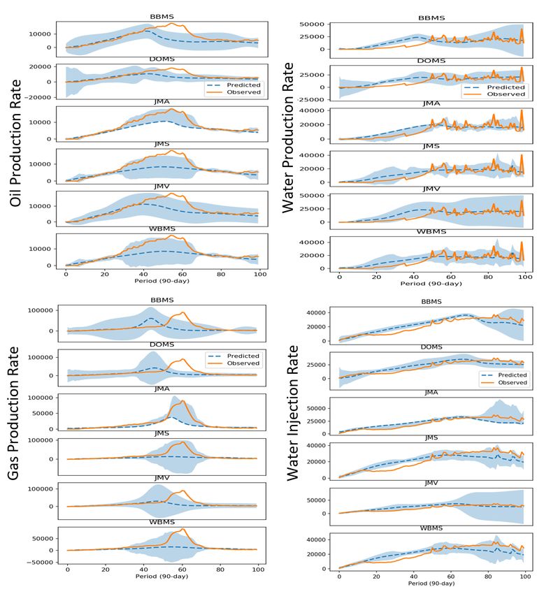
Under review as a conference paper at ICLR 2021

(Engle, 1982), and its generalized version, GARCH, (Bollerslev, 1986) are two such methods, the
latter of which serves as one of our baselines.
An illuminating study (Kendall & Gal, 2017) describes an integration of two sources of uncertainty,
namely the epistemic (due to model) and the aleatoric (due to data). The authors propose a variational
approximation of Bayesian Neural Networks and an implicit Gaussian model to quantify both types
of variability in a non-sequential classification and regression task. Based on Nix & Weigend (1994),
Lakshminarayanan et al. (2017) also uses an implicit Gaussian model to improve the predictive
performance of a base model, again in a non-sequential setting. Similar to Kendall & Gal (2017), the
study does not focus on comparing the quality of the uncertainty to one generated by other methods.
We use the implicit variance model of Kendall & Gal (2017); Oh et al. (2020); Lakshminarayanan
et al. (2017), as well as the method of variational dropout of Gal & Ghahramani (2016); Kendall &
Gal (2017) as baselines in our work. A meta-modeling approach was taken in Chen et al. (2019)
aiming at the task of instance filtering using white-box models. The work relates to ours through
the meta-modeling concept but concentrates on classification in a non-sequential setting. Besides
its application in filtering, meta-modeling has been widely applied in the task of learning to learn
and lifelong learning (Schmidhuber, 1987; Finn et al., 2019). However, it should be pointed out
that the two applications of meta-modeling are not comparable due to their different objectives.
Uncertainty in data drift conditions was assessed in a recent study (Snoek et al., 2019). The authors
employ calibration-based metrics to examine various methods for uncertainty in classification tasks
(image and text data), and conclude, among others that most methods’ quality degrades with drift.
Acknowledging drift as an important experimental aspect, our study takes it into account by testing in
matched and drifted scenarios. Finally, Shen et al. (2018) described a multi-objective training of a
DNN in wind power prediction, minimizing two types of cost related to coverage and bandwidth. We
expand on these metrics in Section 3.3.

3     M ETHOD

3.1   M ETA M ODELING A PPROACH

The basic concept of Meta Modeling (MM), depicted in Figure 1, involves a combination of
two models comprising a base model, performing the main task (e.g., regression), and a meta
model, learning to predict the base model’s error behavior. Depending on the amount of in-
formation shared between these two, we distinguish several settings, namely (1) base model is
a black-box (BB), (2) base is a white-box (WB, base parameters are accessible), and (3) base
and meta components are trained jointly (JM). The advantages of WB and JM are obvious: rich
information is available for the meta model to capture salient patterns for it to generate accu-
rate predictions. On the other hand, the BB setting often occurs in practice and is a given.

We now formalize the MM concept as it applies
to sequential regression. Let ŷ = Fφ (x) be the
base model function parametrized by φ, where
x = x1 , ..., xN and ŷ = ŷ1 , ..., ŷM represent
sequences of N input feature vectors and M D-
dimensional output vectors, with ŷ ∈ RD×M .
Let ẑ = Gγ (ŷ, x, φ) denote the meta model, Figure 1: The concept of meta modeling
parameterized by γ, taking as input the pre-
dictions, the original features, and the parameters of the base to produce a sequence of error
predictions, ẑ ∈ RD×M . The parameters φ are obtained by solving an optimization problem,
                                                                                                     2
arg minφ E[lb (ŷ, y)], using a smooth loss function lb , e.g., the Frobenius norm lb = kŷ − ykF .
Similarly, the parameters γ are determined via arg minγ E[lm (ẑ, z)] = arg minγ E[lm (ẑ, lz (ŷ, y))]
involving a loss lz quantifying the target error (residual) from the base model, and lm quantifying
the prediction error of the meta model. In general, lb , lz , and lm , may differ. The expectations are
estimated using an available dataset. We used the L2F norm for lb and lm , and L1 for lz , as described
in Section 4. Given differentiable loss functions and the DNN setting, the base and the meta model
can be integrated in a single network (JM). In this case the parameters are estimated jointly via

                      φ∗ , γ ∗ = arg min E[βlb (ŷ, y) + (1 − β)lm (ẑ, lz (ŷ, y))]               (1)
                                   φ,γ

                                                    2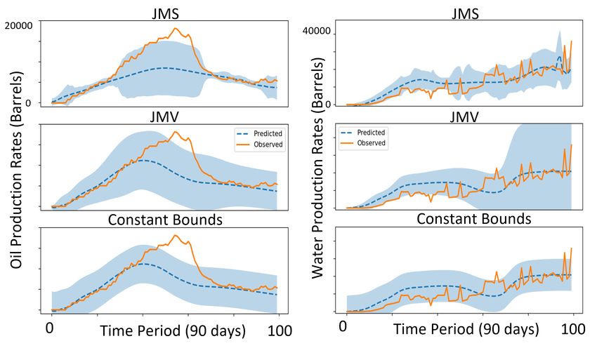
Under review as a conference paper at ICLR 2021

whereby dedicated output nodes of the network generate ŷt and ẑt , and β is a hyper-parameter trading
off the base with the meta loss. Thus, one part of the network tackles the base task, minimizing the
base residual, while another models the residual as the eventual measure of uncertainty. As done in
(Kendall & Gal, 2017), one can argue that the base objective minimizes the epistemic (parametric)
uncertainty, while the meta objective captures the aleatoric uncertainty present in the data. Due to
their interaction, the base loss is influenced by the estimated uncertainty encouraging it to focus
on feature-space regions with lower aleatoric uncertainty. Moreover, we conjecture, the DNN base
model is encouraged to encode the input in ways suitable for uncertainty quantification.
Figure 2 shows an overview of a sequential DNN architecture applied throughout our study. It
includes a base encoder-decoder pair and a meta decoder connected to them. Each of these contains
a recurrent memory cell - the LSTM (Hochreiter & Schmidhuber, 1997). The role of the encoder
is to process the sequential input, x, compress its information in a context vector and pass it to
the base decoder. The recurrent decoder produces the regression output ŷ in M time steps feeding
its predictions as input in the next time steps. Evolving in time, both base LSTMs update their
internal states bt and ht , whereby the last state, bN , serves as the context vector for the decoder. This
architecture has gained wide popularity in applications such as speech-to-text (Chiu et al., 2018;
Tüske et al., 2019), text-to-speech (Sotelo et al., 2017), machine translation (Sutskever et al., 2014),
and image captioning (Rennie et al., 2016). Following the MM concept, we attach an additional
decoder (the meta decoder) via connections to the encoder and decoder outputs. The context vector,
bN , is transformed by a fully connected layer (FCN in Figure 2), and both the ŷt output as well as the
internal state, ht , are fed into the meta component. As mentioned above, the meta decoder generates
uncertainty estimates, ẑt .
Given the architecture depicted in Figure 2, we summarize the three settings as follows:(1) Joint
Model (JM): parameters are trained according to Eq. (1) with certain values of β. (2) White-Box
model (WB): base parameters φ are trained first, followed by parameters γ, also accessing φ. (3)
Black-Box model (BB): same as (2) without access to φ.

                                                             Figure 3: Bandwidth, excess, and deficit
                                                             costs.
Figure 2: Encoder-Decoder architecture integrat-
ing a base and a meta model

Generating Symmetric and Asymmetric Bounds The choice of loss function, lz , gives rise to
two scenarios. If lz is an even function, e.g., lz (ŷ, y) = kŷ − yk1 , the meta-model targets z capture
base error equally in both directions: above and below the target. Hence, the uncertainty ẑ predicted
at test time will represent a interval symmetric around ŷ. If, on the other hand, lz takes the sign
in z into account, it is possible to dedicate separate network nodes γl , γu ∈ γ to capturing lower
and upper band estimates, ẑl and ẑu , respectively, thus accomplishing asymmetric prediction. Let
δ = ŷ − y. For the asymmetric scenario the meta objective is modified as follows:
                    γ ∗ = arg min E[lm (zl , max{δ, 0}) + lm (zu , max{−δ, 0})]                        (2)
                              γ

3.2   BASELINES

Implicit Heteroskedastic Variance Lakshminarayanan et al. (2017); Kendall & Gal (2017); Oh
et al. (2020) applied a Gaussian model N (µ, σ 2 ) to the output of a neural network predictor, where µ

                                                    3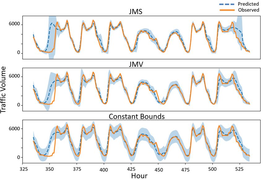
Under review as a conference paper at ICLR 2021

represents the prediction and σ 2 its uncertainty due to observational (aleatoric) noise. The model
is trained to minimize the negative log-likelihood (NLL), with the variance being an implicit un-
certainty parameter (in that it is trained indirectly) which is allowed to vary across the feature
space (heteroskedasticity). We apply the Gaussian in the sequential setting by planting it onto the
base decoder’s output (replacing   the meta decoder) and train    i the network using the NLL objec-
                                        (ŷt,d −yt,d )2
                         hP
        ∗                   M PD                               2
tive: φ = arg minφ E        t=1     d=1       σ2
                                                        + log σt,d with D output nodes modeling the
                                                   t,d

regression variable, ŷt , and separate D output nodes modeling the log σt2 , at time t.

Variational Dropout Gal & Ghahramani (2016) established a connection between dropout (Srivas-
tava et al., 2014), i.e., the process of randomly omitting network connections, and an approximate
Bayesian inference. We apply the variational dropout method to the base encoder and decoder. By
performing multiple runs per test sequence, each with a different random dropout pattern, the base
predictions are calculated as the mean and the base uncertainty as the variance over such runs. This
Bayesian method, along with the variational approximation, captures the parametric (epistemic)
uncertainty of the model, hence it fundamentally differs from the Gaussian model as well as our
proposed approach.

GARCH Variance Introduced in (Bollerslev, 1986; Engle, 1982), the Generalized Autoregressive
Conditional Heteroskedastic (GARCH) variance model belongs among the most popular statistical
methods. A GARCH(p,q) assumes the series to follow an autoregressive moving average model and
                                            combination of past q residual terms, 2 , and p previous
                           Pq t as a linear P
estimates the variance at time
                                              p
variances, σ 2 : σt2 = α0 + i=1 αi 2t−i + i=0 βi σt−i
                                                    2
                                                       .
The α0 term represents a constant component of the variance. The parameters, α, β are estimated via
maximum-likelihood on a training set. The GARCH process relates to the concept in Figure 1 in that
it acts as the meta-model predicting the squared residual. We use the GARCH as a baseline only on
one of the datasets for reasons discussed in Section 4.

Constant-Band Baseline A consistent comparison of uncertainty methods is difficult due to the
fact that each generates an uncertainty around different base predictions. Therefore, as a reference
we also generate a constant symmetric band around each base predictor. Such a bound represents a
homoskedastic process – a sensible choice in many well-behaved sequential regression problems,
corresponding to a GARCH(0,0) model. We will use this reference point to compute a relative gain
of each method as explained in Section 3.3.

3.3   E VALUATION M ETHODOLOGY

Core Metrics Unlike with classification tasks, where standard calibration-based metrics apply
(Snoek et al., 2019), we need to consider two aspects arising in regression, roughly speaking: (1)
what is the extent of observations falling outside the uncertainty bounds (Type 1 cost), and (2) how
excessive are the bounds (Type 2 cost). An optimal bound captures all of the observation while being
least excessive in terms of its bandwidth. Shen et al. (2018), among others, defined two measures
reflecting these aspects (miss rate and bandwidth) which we adopt below (Eqs. (3) and (4)) while
adding two refinements (Eqs. (5) and (6)). Let ŷl = ŷ − ẑl and ŷu = ŷ + ẑu denote the predicted
lower and upper bound, respectively. Recall that ŷ ∈ RD×M . We define the following metrics:
                                                         1       X
                          Missrate(ŷl , ŷu , y) = 1 −                    1                      (3)
                                                        MD           l u  d,t:ydt ∈[ŷdt ,ŷdt ]

                                                                D M
                                                           1 XX u
                          Bandwidth(ŷl , ŷu , y) =                            l
                                                                       ŷdt − ŷdt                        (4)
                                                          2M D
                                                               d=1 t=1
                                           1             X
                Excess(ŷl , ŷu , y) =                                      l     u

                                                               min ydt − ŷdt  , ŷdt − ydt               (5)
                                          MD                l ,ŷ u ]
                                                d,t:ydt ∈[ŷdt   dt

                                          1           X
              Deficit(ŷl , ŷu , y) =                                              l              u

                                                                       min |ydt − ŷdt |, |ydt − ŷdt |   (6)
                                         MD                l ,ŷ u ]
                                              d,t:ydt ∈[ŷ
                                                      / dt      dt

                                                          4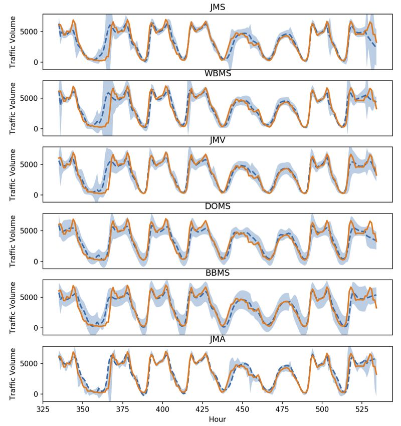
Under review as a conference paper at ICLR 2021

                     Table 1: Overview statistics of the MITV and the SPE9PR datasets

    Dataset         Total         Input        Output       Time                   Partition Size
                   Samples       Features       Dim        Resol.      TRAIN       DEV DEV2             TEST
    MITV            48204           8            1           1 hr       33744       4820     4820       4820
    SPE9PR          28000          248           4         90 days      24000       1000     1000       1000
                    ×100                                                ×100       ×100 ×100            ×100

Figure 3 illustrates these metrics. The relative proportion of observations lying outside the bounds
(miss rate) ignores the extent of the bound’s short fall. The Deficit, Eq. (6), captures this. The type
2 cost is captured by the Bandwidth, Eq. (4). However, its range is indirectly compounded by the
underlying variation in ŷ and y. Therefore we propose the Excess measure, Eq. (5), which also
reflects the Type 2 cost, but just the portion above the minimum bandwidth necessary to include the
observation.

Calibration In general, DNNs offer few guarantees about the behavior of their output. DNNs
tend to produce miscalibrated classification probabilities (Guo et al., 2017). In order to evaluate
the uncertainty across models, it is necessary to establish a common operating point (OP). We
achieve this via a scaling calibration. For symmetric bounds, we assume that y = ŷ + ẑ  where
 ∈ RD×M is a random i.i.d. matrix and ẑ is the predicted non-negative uncertainty band. Let
Zdt = ydtẑ−ŷ
           dt
               dt
                  . Using a held-out dataset, we can obtain an empirical distribution in each output
                                                                                                 (p)
dimension: cdf({Zdt }1≤t≤M ), d = 1, ..., D. It is then possible to find the value εd for a desired
                                                                            h                                  i
                   (0.95)                                                                 (p)              (p)
quantile p, e.g., εd      , and construct the prediction bound at test time: ŷdt − ẑdt εd , ŷdt + ẑdt εd .
Assuming Zd is stationary, in expectation, this bound will contain the desired proportion p of the
observations, i.e., E[Missrate(ŷl , ŷu , y)] = 1 − p.
This scaling is applied in our evaluation to compare the excess, bandwidth and deficit at fixed miss
rates as well as setting a minimum cost OP (see Section 3.3). An Algorithm to find a scale factor for
a desired value of any of the four metrics in O(M 2 ) operations is given in the Appendix.

Metrics Used in Reporting The following OP-based measures are used in reporting: (1) Excess,
Deficit, Bandwidth at a fixed Missrate, averaged over Missrate = {0.1, 0.05, 0.01}, and (2) Minimum
Excess-Deficit cost, where cost = 21 (Excess + Deficit) with the minimum found over all calibrations
(OPs).
For each system and measure, ms , a symmetric constant-band baseline, mf ixed , is also generated
                                                                              m         −ms
and a relative gain with respect to this reference calculated: gains = 100 × fmixed f ixed
                                                                                            %. Finally,
                                                                      1
                                                                        PD   kŷ d −y  k
                                                                                      d 1
the error rate of the base predictor is calculated as Ebase (ŷ, y) = D  d=1    kyd k1 , where ŷd , yd
are d-th row vectors of ŷ, y.

4       E XPERIMENTS

Datasets Two sequential regression datasets, namely the Metro Interstate Traffic Volume (MITV)
dataset1 and the SPE9 Reservoir Production Rates (SPE9PR) dataset2 , were experimented with. Both
originate from real-world applications, involve sequential input/output variables, and provide for
scenarios with varying degrees of difficulty.
The MITV dataset is a collection of hourly weather features with the target of the regression being
the hourly traffic volume, recorded by the Minnesota DoT continuously between 2012 and 2018.
The SPE9PR, on the other hand, is a large collection of mathematical simulations of a reservoir field
with varying input and output sequences with each simulation comprising a sequence with 100 time
steps. The regression targets in this case are multivariate and correspond to field production rates.
    1
        https://archive.ics.uci.edu/ml/machine-learning-databases/00492/
    2
        https://developer.ibm.com/technologies/artificial-intelligence/data/oil-reservoir-simulations

                                                           5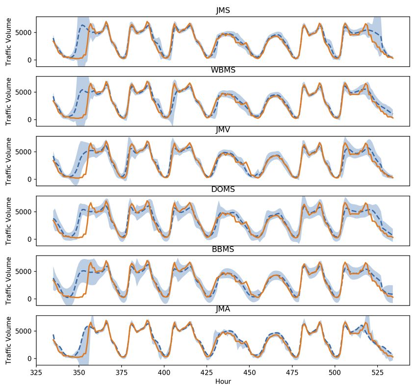
Under review as a conference paper at ICLR 2021

The SPE9PR also contains a data partition collected under distributional drift. Full detail on both
datasets including their preprocessing can be found in the Appendix.

Training Procedure Each dataset was partitioned into TRAIN, DEV, DEV2, and TEST sets (with
SPE9PR also providing a TEST-drift set), as listed Table 1. While the TRAIN/DEV partitions served
basic training, the DEV2 was used in determining hyperparameters and operating points (calibration).
The TEST sets were used to produce the reported metrics. While a single sample in the SPE9PR
represents a complete sequence of 100 steps, the MITV data come as a single contiguous sequence.
The partitioning of the MITV set is strictly ordered by time, whereby the DEV sequence follows
TRAIN, DEV2 follows DEV, and TEST follows DEV2. After partitioning, each MITV sequence
was processed by a sliding window of length 36 hours (in 1-hour steps). This resulted in a series
of (n − 35) × 36 subsequences (n denotes the partition size) to feed the encoder-decoder model.
When testing on the MITV, DNN predictions from such sliding windows were recombined into a
contiguous prediction sequence again.
The base encoder-decoder network (see Figure 2) is trained using the Adam optimizer (Kingma &
Ba, 2014) with a varying initial learning rate, lr, in two stages: (1) Training of all parameters using
TRAIN while providing the ground truth as the decoder input at each time step. (2) Building on the
previous, the training continues, however, decoder predictions from step t − 1 are fed as decoder
inputs at step t—a mode referred to as emulation by Bengio et al. (2015). All hyperparameter values
are listed in the Appendix.

J OINT M ODEL , S YMMETRIC (JMS), AND A SYMMETRIC (JMA): The common training steps are
performed using the objective in Eq. (1), with β = 1.0, first. Then, the joint training continues with
β = 0.5 as long as the objective improves on DEV. In a final step, the model switches to using DEV
as training with β = 0.0 until no improvement on TRAIN is seen. A similar procedure is followed
for the JMA, except using Eq. (2).
W HITE -B OX M ODEL , S YMMETRIC (WBMS): The basic training is performed with β = 1.0.
Next, only meta model parameters are estimated using the DEV/TRAIN sets with β = 0.0.
B LACK -B OX M ODEL , S YMMETRIC (BBMS): Base training is performed. The base model
processes the DEV set to generate residual z. A separate encoder-decoder model is then trained using
(x, z).
J OINT M ODEL WITH VARIANCE (JMV): The two common steps are performed using the NLL
objective (see Section 3.2) with the variance-related parameters first fixed, and, in a subsequent step,
allowing the variance parameters to be adjusted, until convergence. This is to aid stability in training
(Nix & Weigend, 1994).
D ROPOUT M ODEL S YMMETRIC (DOMS): Dropout with a rate of 0.25 (inputs, outputs) and 0.1
(internal states), determined as best performing on the DEV2 set, were applied in both the base
encoder and the decoder. The two common steps were performed. At test time, the model was run 10
times per each test sequence to obtain the mean prediction and standard deviation.
GARCH: The GARCH model from Section 3.2 is used with p = q = 5. The lag value was
determined using an autocorrelation chart showing attenuation at lags > 5. We only apply this
baseline to the MITV dataset as it provides a contiguous time series. The model parameters were
trained using the DEV2 partition.
Throughout the experiments, the size of each LSTM cell was kept fixed at 32 for the base en-
coder/decoder, and at 16 for the meta decoder. The base sizing has been largely driven by our
preliminary study showing it suffices in providing accurate base predictions.

Testing Procedure As mentioned above the SPE9PR dataset has two TEST partitions: one for a
matched and one for a drifted condition. While the MITV dataset does not provide an explicit source
of drift, we induce drift by creating a discrepancy in the modeling procedure between training and
test: In the non-drift condition, the DNN’s decoder is given access to the past 12 hours worth of traffic
observations to make a forecast for the next 24 hours. This is achieved by spanning a 36-hour window
and feeding the decoder inputs the first 12 hours of ground truth, during training. Now to create the
drift scenario we test the MITV model without providing those first 12 hours of observations and the
model uses their own predictions for that period instead. This emulates a “model drift” condition in
that the model, trained to rely on actual observations, is getting its own noisy predictions.

                                                   6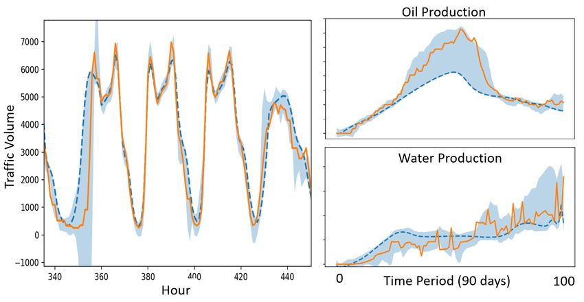
Under review as a conference paper at ICLR 2021
Table 2: Relative optimum and cross-validated gains (G∗ , Gx ) using the Excess-Deficit metrics.
Ebase denotes the base predictor’s error. Within each column, elements marked† are in a statistical
tie, all other values are mutually significant at p < 0.01
MITV SPE9PR
System match Model Drift Match Data Drift
Ebase %G∗ %Gx Ebase %G∗ %Gx Ebase %G∗ %Gx Ebase %G∗ %Gx
JMS .155† 57.8† 59.3† .187† 52.5 55.6 .165 46.5 46.6 .291 56.6 50.5
WBMS .159† 53.8† 55.3† .190† 39.4 42.3 .162 44.8 44.9 .313 54.5 43.8
JMV .167 20.4 25.5 .179 20.0† 17.5† .159 45.3 45.5 .334 -6.5 4.4
DOMS .144 13.2 12.8 .155 16.6† 17.3† .177 1.3 1.4 .279 -0.2 -5.2
BBMS .153† -0.4 1.2 .188† -8.9 -3.0 .170 31.9 30.3 .326 11.6 12.8
GARCH .155† -1.8 3.1 .187† -14.7 -4.0 n/a n/a n/a n/a n/a n/a
Table 3: Relative optimum and cross-validated gains (G∗ and Gx ) on Bandwidth and Excess-Deficit
metrics for the asymmetric JMA model.
MITV SPE9PR
Evaluation Match Drift Match Drift
JMA Base Error .158 .200 .168 .320
JMA, %G∗
Ex-Deficit Bandwidth
44.1 37.0 35.5 54.3
JMA, %Gx 33.1 26.4 35.5 8.5
JMS, %G∗ 37.5 31.6 29.1 34.3
JMS, %Gx 35.2 27.2 28.7 -4.4
JMA, %G∗ 45.3 29.0 30.9 50.8
JMA, %Gx 40.4 28.6 30.8 24.2
JMS, %G∗ 57.8 52.5 46.5 56.6
JMS, %Gx 59.3 55.6 46.6 50.5
Results with Symmetric Bounds Table 2 compares the proposed symmetric-bounds systems (JMS,
WBMS, BBMS) with the baselines (JMV, DOMS, GARCH). The relative error of the base predictor
is given in the Ebase column. The uncertainty quality is reported in Table 2 is the average gain in
excess-deficit metrics, as defined in Section 3.3. Columns labeled as G∗ contain measurements made
at an operating point (OP) determined on the test set itself, while those labeled as Gx use an OP from
a held-out (DEV2) set. While Gx reflects generalization of the calibration, G∗ values are interesting
as they reveal the potential of each method. Based on a paired permutation test (Dwass, 1957) all but
entries marked with † are mutually significant at p < 0.01.
From Table 2 we make the following observations: (1) the JMS model dominates all other models
across all conditions. The fact that it outperforms the WBMS indicates there is a benefit to the
joint training setup, as conjectured earlier. (2) The WBMS dramatically outperforms the BBMS
model, which remains only as good as a constant band for MITV data, indicating it is hard to reliably
predict residuals from only the input features. (3) The most competitive baseline is the JMV model.
As discussed in Section 3.2, the JMV shares some similarity with the meta-modeling approach.
(4) The JMS and WBMS models perform particularly well in the strong drift scenario (SPE9PR),
suggesting that white-box features play an essential role in achieving generalization. Finally, (5) the
DOMS model works well on MITV data but provides no benefit in the SPE9PR, which could be due
the aleatoric uncertainty playing a dominant role in this dataset. In almost all cases, however, the
averaging of base predictions in DOMS results in lowest error rates of the base predictor.
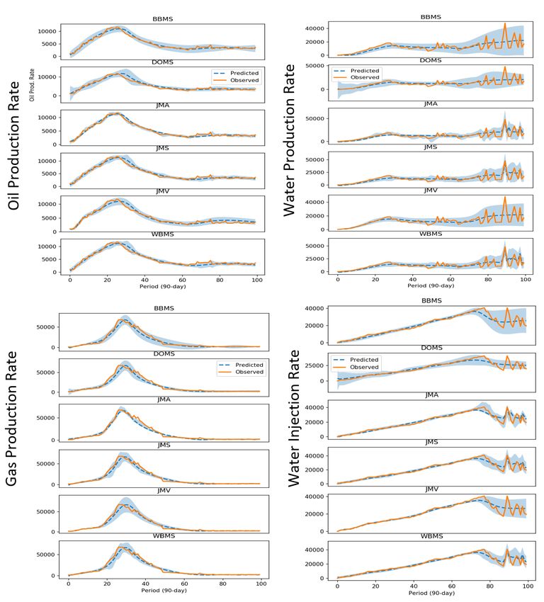
Representative samples of JMS and JMV uncertainty bounds are shown in Figure 4 (MITV) and
Figure 5 (SPE9PR). They illustrate a clear trend in the results, namely that the JMS (also seen with
WBMS) model are better able to cover the actual observation, particularly when the base prediction
tends to make large errors. Additional plots can be found in the Appendix, and also a notebook to
visualize all test samples is provided as part of the Supplementary Material.
Results with Asymmetric Bounds Generating asymmetric bounds is a new intriguing aspect of
DNN-based meta-models. Using the JMA model, we first recorded the accuracy with which the
7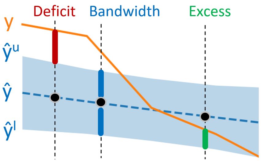
Under review as a conference paper at ICLR 2021

Figure 4: Sample of traffic volume predictions with uncertainty generated by the JMS and JMV
models, along with a constant bound (around JMV) (miss rate set to 0.1 on TEST).

Figure 5: SPE9PR samples of oil (left) and water (right) production rates (”drift” scenario, miss rate
set to 0.1 on TEST).

Figure 6: Samples of asymmetric bounds produced by the JMA. MITV sample (left) and SPE9PR
(right) correspond to segments shown in Figure 4 and 5.

                                                  8
Under review as a conference paper at ICLR 2021
asymmetric output agrees in sign (orientation) with the observed base discrepancy. Averaged over
each of the two datasets, this accuracy is at 83.3%, and 91.1%. The promise of asymmetric bounds
lies in its potential to reduce the bandwidth cost. Since the Excess and Deficit metrics ignore the
absolute bandwidth, we also evaluate the JMA model using the Bandwidth metric (Eq. (4)), averaged
over the same OPs. The results are shown in Table 3 comparing the JMA model to the best symmetric
model, JMS. The JMS model outperforms JMA in all scenarios on Excess-Deficit, however, compared
on the bandwidth metric, the JMA dominates benefiting from its orientation capability. Upon visual
inspection the output of the JMA is appreciably better in bandwidth: Figure 6 shows samples on both
datasets. In most instances the bounds behave as expected, expending the bulk of bandwidth in the
correct direction. An interesting question arises whether it is possible to utilize the asymmetric output
as a correction on the base predictor. Our preliminary investigation shows that a naive combination
leads to degradation in the base error, however, this question remains of interest for future work.
5 C ONCLUSIONS
In this work we demonstrated that meta-modeling (MM) provides a powerful new framework for
uncertainty prediction. Through a systematic evaluation of the proposed MM variants we report
considerable relative gains over a constant reference baseline and show that they not only outperform
all competitive baselines but also show stability across drift scenarios. A jointly trained model
integrating the base with a meta component fares best, followed by a white-box setup, indicating that
trainable white-box features play an essential role in the task. Besides symmetric uncertainty, we
also investigated generating asymmetric bounds using dedicated network nodes and showed their
benefit in reducing the uncertainty bandwidth. We believe these results open an exciting new research
avenue for uncertainty quantification in sequential regression.
R EFERENCES
M. Arnold, R. K. E. Bellamy, M. Hind, S. Houde, S. Mehta, A. Mojsilović, R. Nair, K. N. Ra-
mamurthy, A. Olteanu, D. Piorkowski, D. Reimer, J. Richards, J. Tsay, and K. R. Varshney.
Factsheets: Increasing trust in ai services through supplier’s declarations of conformity. IBM
Journal of Research and Development, 63(4/5):6:1–6:13, July 2019. ISSN 0018-8646. doi:
10.1147/JRD.2019.2942288.
E. Begoli, T. Bhattacharya, and D Kusnezov. The need for uncertainty quantification in machine-
assisted medical decision making. Nature Mach Intell, 1:20–23, 2019.
Samy Bengio, Oriol Vinyals, Navdeep Jaitly, and Noam Shazeer. Scheduled sampling for sequence
prediction with recurrent neural networks. In Proceedings of the 28th International Conference
on Neural Information Processing Systems - Volume 1, NIPS15, pp. 11711179, Cambridge, MA,
USA, 2015. MIT Press.
Tim Bollerslev. Generalized autoregressive conditional heteroskedasticity. Journal of Econometrics,
31(3):307–327, April 1986.
Tongfei Chen, Jiřı́ Navrátil, Vijay Iyengar, and Karthikeyan Shanmugam. Confidence scoring using
whitebox meta-models with linear classifier probes. In The 22nd International Conference on
Artificial Intelligence and Statistics, AISTATS 2019, 16-18 April 2019, Naha, Okinawa, Japan, pp.
1467–1475, 2019.
C. Chiu, T. N. Sainath, Y. Wu, R. Prabhavalkar, P. Nguyen, Z. Chen, A. Kannan, R. J. Weiss, K. Rao,
E. Gonina, N. Jaitly, B. Li, J. Chorowski, and M. Bacchiani. State-of-the-art speech recognition
with sequence-to-sequence models. In 2018 IEEE International Conference on Acoustics, Speech
and Signal Processing (ICASSP), pp. 4774–4778, April 2018.
Meyer Dwass. Modified randomization tests for nonparametric hypotheses. Ann. Math. Statist., 28
(1):181–187, 03 1957. doi: 10.1214/aoms/1177707045.
Robert F. Engle. Autoregressive conditional heteroscedasticity with estimates of the variance of
united kingdom inflation. Econometrica, 50(4):987–1007, 1982. ISSN 00129682, 14680262.
9Under review as a conference paper at ICLR 2021
Chelsea Finn, Aravind Rajeswaran, Sham Kakade, and Sergey Levine. Online meta-learning. In
Kamalika Chaudhuri and Ruslan Salakhutdinov (eds.), Proceedings of the 36th International
Conference on Machine Learning, volume 97 of Proceedings of Machine Learning Research, pp.
1920–1930, Long Beach, California, USA, 09–15 Jun 2019. PMLR.
Yarin Gal and Zoubin Ghahramani. A theoretically grounded application of dropout in recurrent
neural networks. In D. D. Lee, M. Sugiyama, U. V. Luxburg, I. Guyon, and R. Garnett (eds.),
Advances in Neural Information Processing Systems 29, pp. 1019–1027. Curran Associates, Inc.,
2016.
Chuan Guo, Geoff Pleiss, Yu Sun, and Kilian Q. Weinberger. On calibration of modern neural
networks. In Proceedings of the 34th International Conference on Machine Learning - Volume 70,
ICML17, pp. 13211330. JMLR.org, 2017.
Sepp Hochreiter and Jürgen Schmidhuber. Long short-term memory. Neural Comput., 9(8):17351780,
November 1997. ISSN 0899-7667. doi: 10.1162/neco.1997.9.8.1735.
Heinrich Jiang, Been Kim, Melody Guan, and Maya Gupta. To trust or not to trust a classifier.
In S. Bengio, H. Wallach, H. Larochelle, K. Grauman, N. Cesa-Bianchi, and R. Garnett (eds.),
Advances in Neural Information Processing Systems 31, pp. 5541–5552. Curran Associates, Inc.,
2018.
Alex Kendall and Yarin Gal. What uncertainties do we need in bayesian deep learning for computer
vision? In I. Guyon, U. V. Luxburg, S. Bengio, H. Wallach, R. Fergus, S. Vishwanathan, and
R. Garnett (eds.), Advances in Neural Information Processing Systems 30, pp. 5574–5584. Curran
Associates, Inc., 2017.
J.E. Killough. Ninth SPE comparative solution project: A reexamination of black-oil simulation.
In SPE Reservoir Simulation Symposium. Society of Petroleum Engineers, 1995. doi: 10.2118/
29110-ms.
Diederik P. Kingma and Jimmy Ba. Adam: A method for stochastic optimization, 2014. cite
arxiv:1412.6980Comment: Published as a conference paper at the 3rd International Conference for
Learning Representations, San Diego, 2015.
Balaji Lakshminarayanan, Alexander Pritzel, and Charles Blundell. Simple and scalable predictive
uncertainty estimation using deep ensembles. In I. Guyon, U. V. Luxburg, S. Bengio, H. Wallach,
R. Fergus, S. Vishwanathan, and R. Garnett (eds.), Advances in Neural Information Processing
Systems 30, pp. 6402–6413. Curran Associates, Inc., 2017.
Aleksander Madry, Aleksandar Makelov, Ludwig Schmidt, Dimitris Tsipras, and Adrian Vladu.
Towards deep learning models resistant to adversarial attacks. ArXiv, abs/1706.06083, 2017.
Terence C. Mills. Time Series Techniques for Economists. Number 9780521405744 in Cambridge
Books. Cambridge University Press, 1991.
D. A. Nix and A. S. Weigend. Estimating the mean and variance of the target probability distribution.
In Proceedings of 1994 IEEE International Conference on Neural Networks (ICNN’94), volume 1,
pp. 55–60 vol.1, June 1994. doi: 10.1109/ICNN.1994.374138.
Min-hwan Oh, Peder A. Olsen, and Karthikeyan Natesan Ramamurthy. Crowd counting with
decomposed uncertainty. In AAAI Conference on Artificial Intelligence, 2020.
A. Papoulis and H. Saunders. Probability, Random Variables and Stochastic Processes (2nd Edition).
Journal of Vibration, Acoustics, Stress, and Reliability in Design, 111(1):123–125, 01 1989. ISSN
0739-3717. doi: 10.1115/1.3269815.
Steven J. Rennie, Etienne Marcheret, Youssef Mroueh, Jerret Ross, and Vaibhava Goel. Self-critical
sequence training for image captioning. CoRR, abs/1612.00563, 2016.
Jurgen Schmidhuber. Evolutionary principles in self-referential learning. on learning now to learn:
The meta-meta-meta...-hook. Diploma thesis, Technische Universitat Munchen, Germany, 14 May
1987. URL http://www.idsia.ch/˜juergen/diploma.html.
10Under review as a conference paper at ICLR 2021
Yanxia Shen, Xu Wang, and Jie Chen. Wind power forecasting using multi-objective evolutionary
algorithms for wavelet neural network-optimized prediction intervals. Applied Sciences, 8(2):185,
Jan 2018. ISSN 2076-3417. doi: 10.3390/app8020185.
Jasper Snoek, Yaniv Ovadia, Emily Fertig, Balaji Lakshminarayanan, Sebastian Nowozin, D Sculley,
Joshua Dillon, Jie Ren, and Zachary Nado. Can you trust your model’s uncertainty? evaluating
predictive uncertainty under dataset shift. In Advances in Neural Information Processing Systems,
pp. 13969–13980, 2019.
Jose Sotelo, Soroush Mehri, Kundan Kumar, João Felipe Santos, Kyle Kastner, Aaron C. Courville,
and Yoshua Bengio. Char2wav: End-to-end speech synthesis. In 5th International Conference
on Learning Representations, ICLR 2017, Toulon, France, April 24-26, 2017, Workshop Track
Proceedings, 2017.
Nitish Srivastava, Geoffrey Hinton, Alex Krizhevsky, Ilya Sutskever, and Ruslan Salakhutdinov.
Dropout: A simple way to prevent neural networks from overfitting. Journal of Machine Learning
Research, 15:1929–1958, 2014.
Ilya Sutskever, Oriol Vinyals, and Quoc V. Le. Sequence to sequence learning with neural networks.
In Proceedings of the 27th International Conference on Neural Information Processing Systems -
Volume 2, NIPS14, pp. 31043112, Cambridge, MA, USA, 2014. MIT Press.
Zoltán Tüske, Kartik Audhkhasi, and George Saon. Advancing sequence-to-sequence based speech
recognition. Proc. Interspeech 2019, pp. 3780–3784, 2019.
11Under review as a conference paper at ICLR 2021
Algorithm 1 Find best scale for a given metric value
Input: Observation, base and meta predictions {ŷt , yt , ẑtl , ẑtu }1≤t≤M ; metric function f ; target
value ρ∗
Output: Scale factor ε∗
for t ← 1 to M do
δt ← ŷ(t − yt .
δt
l for δt ≥ 0
εt ← ẑ−δ t
ẑtu
t
otherwise
for k ← 1 to M do
ŷkl ← ŷk − εt ẑkl
ŷku ← ŷk − εt ẑku
end for
ρt ← f ŷkl , ŷku , yk 1≤k≤M
end for
t∗ ← arg mint |ρt − ρ∗ |
ε∗ ← εt∗
A A LGORITHM TO F IND A S CALING FACTOR
Section 3.3 discusses the scaling calibration in the context of the four metrics: Missrate, Bandwidth,
Excess, and Deficit. Algorithm 1 finds a scale factor for a desired value of any of these four metrics
in O(M 2 ) operations.
B A DDITIONAL DATASET AND I MPLEMENTATION D ETAILS
B.1 DATASETS
B.1.1 M ETRO I NTERSTATE T RAFFIC VOLUME (MITV)
The dataset is a collection of hourly westbound-traffic volume measurements on Interstate 94 reported
by the Minnesota DoT ATR station 301 between the years 2012 and 2018. These measurements are
aligned with hourly weather features3 as well as holiday information, also part of the dataset. The
target of regression is the hourly traffic volume. This dataset was released in May, 2019.
The MITV input features were preprocessed to convert all categorical features to trainable vector
embeddings, as outlined in Figure 2. All real-valued features as well as the regression output
were standardized before modeling (with the test predictions restored to their original range before
calculating final metrics). Overall dataset statistics are listed in Table 1 and further processing steps
are given in Section 4.
B.1.2 MITV P RE P ROCESSING
As described in Section B.1.1 and Table 1, the MITV dataset comes with 8 input features, among
which 3 are categorical. Here we list the relevant parsing and encoding steps used in our setup.
The raw time stamp information was parsed to extract additional features such as day of the week,
day of the month, year-day fraction, etc. Table 4 shows the corresponding list. Standardization
was performed on the input as well as output, as per Table 4, whereby the model predictions were
transformed to their original range before calculating final metrics.
B.1.3 SPE9 R ESERVOIR P RODUCTION R ATES (SPE9PR)
This dataset originates from an application of oil reservoir modeling. A reservoir model (RM) is a
space-discretized approximation of a geological region subject to modeling. Given a sequence of
drilling actions (input), a physics-based PDE-solver (simulator) is applied to the RM to generate
3
provided by OpenWeatherMap
12Under review as a conference paper at ICLR 2021
Table 4: MITV Input and Output Specifications
Feature Range Categorical Embedding Standardized Final
Name Dimension Dimension
INPUT
day of month integer ∈ [0, 30] Y 3 N 3
day of week integer ∈ [0, 6] Y 3 N 3
month integer ∈ [0, 11] Y 3 N 3
1
frac yday real ∈ [ 365 , 1] N - Y 1
weather type integer ∈ [0, 10] Y 3 N 3
holiday type integer ∈ [0, 11] Y 3 N 3
temperature real ∈ R N - Y 1
rain 1h real ∈ R+ 0 N - Y 1
snow 1h real ∈ R+ 0 N - Y 1
clouds all real ∈ [0, 100] N - Y 1
Total 20
OUTPUT
traffic volume real ∈ R+
0 N - Y 1
Total 1
sequences of future production rates (oil, gas, water production), typically over long horizons Killough
(1995). The objective is to train a DNN and accurately predict outputs on unseen input sequences.
We used the publicly available SPE94 RM, considered a reference for benchmarking reservoir
simulation in the industry, and an open-source simulator5 to produce 28,000 simulations, each with
100 randomized actions (varying type, location, and control parameters of a well) inducing production
rate sequences over a span of 25 years, in 90-day increments, i.e., 100 time steps. Furthermore, the
RM was partitioned into two regions, A and B. While most of the actions are located in the region A,
we also generated 1000 sequences with actions located in the region B thus creating a large degree
of mismatch between training and test. The test condition in region B will be referred to as “drift”
scenario.
B.1.4 SPE9PR P RE P ROCESSING
The Table 5 lists details on the SPE9PR features (also refer to Section B.1.3 and Table 1). The
SPE9PR dataset contains input sequences of actions and output sequences of production rates. An
action (feature type of well), at a particular time, represents a decision whether to drill, and if so,
what type of well to drill (an injector or a producer well), or not to drill (encoded by ”0”), hence the
cardinality is 3. In case of a drill decision, further specifications apply, namely the x- and y-location
on the surface of the reservoir, local geological features at the site, and well control parameters.
There are 15 vertical cells in the SPE9 each coming with 3 geological features (rel. permeability, rel.
porosity, rock type), thus the local geology is a 45-dimensional feature vector at a particular (x, y)
location. Finally, every well drilled so far may be controlled by a parameter called ”Bottom-Hole
Pressure” (BHP). Since we provision up to 100 wells of each of the two types, a 200-dimensional
vector arises containing BHP values for these wells at any given time. Standardization was performed
on the input as well as output as specified in Table 5 whereby the model predictions were transformed
to their original range before calculating and reporting final metrics.
4
https://github.com/OPM/opm-data/blob/master/spe9/SPE9.DATA
5
https://opm-project.org/
13Under review as a conference paper at ICLR 2021
Table 5: SPE9PR Input and Output Specifications
Feature Range Categorical Embedding Standardized Final
Name Dimension Dimension
INPUT
type of well integer ∈ {0, 1, 2} Y 3 N 3
location x integer ∈ [0, 24] Y 10 N 10
location y integer ∈ [0, 25] Y 10 N 10
vertical geology real ∈ R45 N - Y 45
per well control real ∈ R200 N - Y 200
Total 258
OUTPUT
oil prod field rate real ∈ R+
0 N - Y 1
gas prod field rate real ∈ R+
0 N - Y 1
water prod field rate real ∈ R+
0 N - Y 1
water inj field rate real ∈ R+
0 N - Y 1
Total 4
Table 6: Hyperparameter settings
Hyper- Where Value Comment
parameter used
Learning rate all 0.001 Stage 1 training
Learning rate all 0.0002 Stage 2 training, see Section 4
Batch size all 100
L2 penalty coefficient all, except DOMS 0.0001
L2 penalty coefficient DOMS 0.0
Dropout DOMS 0.25/0.1/0.25 LSTM Input/State/Output (encoder and decoder)
Base LSTM size all 32
Meta LSTM size meta models 16
β in Eq. (1) 1.0/0.5/0.0 see Section 4
B.2 T RAINING S ETUP
B.2.1 H YPERPARAMETERS
Hyperparameters have been determined in two ways: (1) learning rate, regularization, batch, and
LSTM size were adopted from an unrelated experimental study performed on a modified reservoir
SPE9 (Anonymized), (2) We used DEV2 to determine the dropout rates in the DOMS model. The
value β = 0.5 was chosen ad-hoc (as a midpoint between pure base and pure meta loss) without
further optimization.
B.3 I MPLEMENTATION N OTES
All DNNs were implemented in Tensorflow 1.11. Training was done on a Tesla K80 GPU, with
total training time ranging between 3 (MITV) and 24 (SPE9PR) hours. The GARCH Python
implementation provided in the arch library was used.
14Under review as a conference paper at ICLR 2021
Table 7: Relative optimum and cross-validated gains (G∗ , Gxval ) for the MITV dataset, using the
Excess-Deficit metrics. Ebase denotes the base predictor’s error. Within each column, elements
marked† are in a statistical tie, all other values are mutually significant at p < 0.01
MITV
System match drift
Ebase %G∗ %Gxval Ebase %G∗ %Gxval
JMS .155† 57.8† 59.3† .187† 52.5 55.6
† † †
WBMS .159 53.8 55.3 .190† 39.4 42.3
JMV .167 20.4 25.5 .179 20.0† 17.5†
DOMS .144 13.2 12.8 .155 16.6† 17.3†
† †
BBMS .153 -0.4 1.2 .188 -8.9 -3.0
GARCH .155† -1.8 3.1 .187† -14.7 -4.0
Table 8: Relative optimum and cross-validated gains (G∗ , Gxval ) for the SPE9PR dataset, using
the Excess-Deficit metrics. Ebase denotes the base predictor’s error. Within each column, elements
marked† are in a statistical tie, all other values are mutually significant at p < 0.01
SPE9PR
System match drift
Ebase %G∗ %Gxval Ebase %G∗ %Gxval
JMS .165 46.5 46.6 .291 56.6 50.5
WBMS .162 44.8 44.9 .313 54.5 43.8
JMV .159 45.3 45.5 .334 -6.5 4.4
DOMS .177 1.3 1.4 .279 -0.2 -5.2
BBMS .170 31.9 30.3 .326 11.6 12.8
C A DDITIONAL R ESULTS
C.1 I NDIVIDUAL M ETRICS
For a more detailed view of the averages in Table 2, we show a split by the individual metrics in Table
9, and, for the SPE9PR which has a total of four output variables, a split by the individual variables
in Table 10.
C.2 A DDITIONAL V ISUALIZATIONS
In addition to the sample visualizations shown in Section 2 for the JMS, JMV, and JMA systems,
here we show same sections of the data and visualize output of all systems. Figures 7 and 8 show the
first simulation in the test set of the SPE9PR dataset for the drift and non-drift condition and all its
output components, respectively. Figures 9 and 10 show the output on the MITV drift and non-drift
condition, respectively. For each model, a miss rate value of 0.1 across the entire test set was used in
the visualizations.
C.2.1 I NTERACTIVE N OTEBOOK
We also provide an interactive notebook that allows for inspecting all system output on an arbitrary
portion of the test data in both the non-drift and drift condition. Please refer to the README file
within the zip-file uploaded as the Supplementary Material part of our submission.
C.2.2 JMV VARIANCE T UNING ON DEV DATA
Section 4 lists individual training steps for each system. It is noted that the meta-modeling arrange-
ments have used the DEV partition for tuning in a final step. The motivation for using a partition not
included in training the base model is the avoidance of meta-training on biased targets, i.e., targets
generated by the base model on its own training data. In this context, a question arises whether a sim-
15Under review as a conference paper at ICLR 2021
Figure 7: Sample from SPE9PR (simulation 0, drift condition), all components and systems shown.
16Under review as a conference paper at ICLR 2021
Figure 8: Sample from SPE9PR (simulation 0, non-drift condition), all components and all systems
shown.
17Under review as a conference paper at ICLR 2021
Figure 9: Sample from MITV (drift condition), all systems shown.
18Under review as a conference paper at ICLR 2021
Figure 10: Sample from MITV (non-drift condition), all systems shown.
19Under review as a conference paper at ICLR 2021
ilar tuning step could help the JMV model. We followed the training steps described in Section 4 and
then updated the network nodes tied to the variance parameter while keeping the rest of the network
fixed. The Table 11 shows the results on the MITV dataset. It seems the benefit of the tuning step
does not materialize. In all but the cross-validated drift case the gain decreases (albeit insignificantly)
when applying the DEV-only tuning. We conjecture that the benefit of the tuning step exists with
the meta-model because of the direct supervision of the meta-model’s prediction. In contrast, the
variance in the JMV setting is learned implicitly and may not suffer from the ”biased-target” problem
mentioned above.
20Under review as a conference paper at ICLR 2021
Table 9: Symmetric gains split by individual metric (compare to Table 2)
Model Deficit@0.01 Deficit@0.05 Deficit@0.1 Excess@0.01 Excess@0.05 Excess@0.1 MinCost Average
%G∗ , MITV ”Non-Drift” Scenario
JMS 61.3 74.8 75.6 64.5 54.6 40.1 33.9 57.8
WBMS 48.0 73.8 74.3 62.7 50.7 35.1 32.3 53.8
JMV -33.9 31.9 32.5 35.8 31.4 28.2 16.8 20.4
DOMS 28.1 24.8 23.1 11.5 3.3 -1.6 2.8 13.1
BBMS 9.7 27.9 16.3 -18.8 -18.7 -18.7 -0.8 -0.4
%Gxval , MITV ”Non-Drift” Scenario
JMS 75.9 78.1 77.4 58.0 51.9 39.6 33.9 59.3
WBMS 67.4 79.6 77.7 57.7 42.7 29.8 32.3 55.3
JMV 4.4 38.9 35.8 29.1 27.1 26.3 16.8 25.5
DOMS 78.2 63.9 62.3 -35.7 -32.4 -49.2 2.8 12.8
BBMS 61.6 21.5 15.4 -61.0 -12.5 -15.9 -0.9 1.2
%G∗ , MITV ”Drift” Scenario
JMS 40.5 78.0 77.5 57.7 45.0 31.9 36.7 52.5
WBMS 18.4 68.8 70.8 43.6 32.8 15.6 25.8 39.4
JMV -3.8 29.0 30.9 23.0 25.5 21.6 13.8 20.0
DOMS 23.4 23.7 24.7 11.6 14.2 11.4 7.3 16.6
BBMS -38.2 5.7 8.7 -11.8 -12.2 -14.1 -0.2 -8.9
%Gxval , MITV ”Drift” Scenario
JMS 71.7 81.6 80.1 53.2 39.1 27.1 36.7 55.6
WBMS 67.9 79.2 78.5 22.9 19.4 2.0 25.8 42.3
JMV -27.2 28.5 32.7 29.1 25.9 19.6 13.8 17.5
DOMS 38.4 18.9 23.4 2.8 16.6 13.3 7.4 17.3
BBMS 6.2 13.2 13.1 -17.5 -17.4 -18.6 -0.3 -3.0
%G∗ , SPE9PR ”Non-Drift” Scenario
JMS 55.7 55.8 56.8 46.1 42.5 37.7 30.8 46.5
WBMS 50.9 54.5 55.6 47.4 41.5 35.4 28.5 44.8
JMV 50.5 54.2 53.7 51.8 43.3 37.0 26.4 45.3
DOMS 7.1 10.2 10.4 -6.9 -5.8 -6.8 1.0 1.3
BBMS 51.0 52.6 50.0 25.1 18.2 10.6 15.7 31.9
%Gxval , SPE9PR ”Non-Drift” Scenario
JMS 56.8 56.5 57.0 45.7 42.0 37.4 30.8 46.6
WBMS 50.7 54.9 56.2 47.5 41.2 34.9 28.5 44.8
JMV 51.4 56.0 55.2 51.6 42.3 35.5 26.4 45.5
DOMS 7.7 9.5 10.1 -7.0 -5.3 -6.4 1.0 1.4
BBMS 76.4 61.2 54.8 -11.5 10.6 5.0 15.7 30.3
%G∗ , SPE9PR ”Drift” Scenario
JMS 65.4 69.0 68.4 52.6 50.0 46.3 44.5 56.6
WBMS 63.7 68.0 66.9 53.5 48.1 41.8 39.5 54.5
JMV 29.2 22.7 21.9 -33.9 -42.8 -52.9 10.3 -6.5
DOMS -1.4 9.4 12.0 -10.7 -4.5 -8.5 2.7 -0.1
BBMS 19.4 33.8 31.0 -7.6 1.1 -3.0 6.7 11.6
%Gxval , SPE9PR ”Drift” Scenario
JMS 95.0 85.5 78.7 22.8 18.8 14.4 38.5 50.5
WBMS 94.7 84.1 77.3 16.8 5.0 -5.9 34.9 43.8
JMV -40.0 -25.2 -12.2 48.3 31.6 16.9 11.3 4.4
DOMS 16.4 10.1 9.1 -23.4 -23.5 -26.9 1.8 -5.2
BBMS 40.5 9.4 7.9 0.8 17.3 9.0 5.0 12.8
21Under review as a conference paper at ICLR 2021
Table 10: Symmetric gains split by individual components - SPE9PR only (compare to Table 2).
OPR=Oil Production Rate, WPR=Water Production Rate, GPR=Gas Production Rate, WIN=Water
Injection Rate.
Ebase Excess-Deficit
Model OPR WPR GPR WIN Average OPR WPR GPR WIN Average
%G∗ , SPE9PR ”Non-Drift” Scenario
JMS 0.12 0.28 0.17 0.09 0.17 18.25 66.45 53.60 47.61 46.48
WBMS 0.12 0.28 0.17 0.09 0.16 17.78 62.08 52.43 47.03 44.83
JMV 0.10 0.29 0.16 0.09 0.16 6.67 74.50 43.74 56.24 45.29
DOMS 0.12 0.31 0.18 0.11 0.18 -6.88 0.68 21.64 -10.16 1.32
BBMS 0.12 0.30 0.16 0.10 0.17 -3.85 74.44 16.89 40.08 31.89
%G∗ , SPE9PR ”Non-Drift” Scenario
JMS 0.12 0.28 0.17 0.09 0.17 19.13 66.98 52.18 48.19 46.62
WBMS 0.12 0.28 0.17 0.09 0.16 18.32 62.60 51.07 47.39 44.85
JMV 0.10 0.29 0.16 0.09 0.16 6.92 75.74 43.12 56.23 45.50
DOMS 0.12 0.31 0.18 0.11 0.18 -6.56 0.46 21.94 -10.27 1.39
BBMS 0.12 0.30 0.16 0.10 0.17 -3.84 76.80 7.71 40.63 30.33
%G∗ , SPE9PR ”Drift” Scenario
JMS 0.28 0.30 0.45 0.13 0.29 49.97 24.13 119.73 32.54 56.59
WBMS 0.31 0.34 0.45 0.14 0.31 51.49 27.09 102.64 36.77 54.50
JMV 0.30 0.32 0.51 0.20 0.33 1.12 -6.18 26.99 -47.96 -6.51
DOMS 0.28 0.28 0.45 0.11 0.28 -20.24 -6.97 22.32 4.31 -0.15
BBMS 0.32 0.31 0.54 0.13 0.33 -4.18 -1.04 26.64 25.13 11.64
%Gxval , SPE9PR ”Drift” Scenario
JMS 0.28 0.30 0.45 0.13 0.29 61.81 39.10 74.23 27.01 50.54
WBMS 0.31 0.34 0.45 0.14 0.31 59.11 34.21 60.51 21.51 43.84
JMV 0.30 0.32 0.51 0.20 0.33 2.15 9.15 19.51 -13.28 4.38
DOMS 0.28 0.28 0.45 0.11 0.28 0.81 -27.32 15.73 -10.09 -5.22
BBMS 0.32 0.31 0.54 0.13 0.33 2.55 4.67 20.74 23.36 12.83
Table 11: Relative optimum and cross-validated gains using Excess-deficit metrics for the JMV
system without (JMV) and with (JMV-σ) variance tuning on DEV. Elements marked† within same
column are in a statistical tie.
Evaluation %G∗ %Gx
JMV (Drift) 20.0 17.5†
JMV-σ (Drift) 15.0 19.4†
JMV (Match) 20.4† 25.5
JMV-σ (Match) 16.2† 16.9.
22You can also read