Generation of the exact Pareto set in multi-objective traveling salesman and set covering problems
←
→
Page content transcription
If your browser does not render page correctly, please read the page content below
Munich Personal RePEc Archive

Generation of the exact Pareto set in
multi-objective traveling salesman and
set covering problems

Florios, Kostas and Mavrotas, George

National Technical University of Athens

15 June 2014

Online at https://mpra.ub.uni-muenchen.de/105074/
MPRA Paper No. 105074, posted 01 Jan 2021 12:59 UTC
Generation of the exact Pareto set in multi-objective traveling
                   salesman and set covering problems

                                     Kostas Florios, George Mavrotas1
                  Laboratory of Industrial and Energy Economics, School of Chemical Engineering,
                National Technical University of Athens, Zographou Campus, Athens 15780, Greece
                                    Tel: +30 210-7723202, fax: +30 210 7723155

Abstract: The calculation of the exact set in Multi-Objective Combinatorial Optimization (MOCO) problems is one
of the most computationally demanding tasks as most of the problems are NP-hard. In the present work we use
AUGMECON2 a Multi-Objective Mathematical Programming (MOMP) method which is capable of generating the
exact Pareto set in Multi-Objective Integer Programming (MOIP) problems for producing all the Pareto optimal
solutions in two popular MOCO problems: The Multi-Objective Traveling Salesman Problem (MOTSP) and the
Multi-Objective Set Covering problem (MOSCP). The computational experiment is confined to two-objective
problems that are found in the literature. The performance of the algorithm is slightly better to what is already found
from previous works and it goes one step further generating the exact Pareto set to till now unsolved problems. The
results are provided in a dedicated site and can be useful for benchmarking with other MOMP methods or even
Multi-Objective Meta-Heuristics (MOMH) that can check the performance of their approximate solution against the
exact solution in MOTSP and MOSCP problems.

Keywords: multi-objective, traveling salesman problem, set covering problem, ε-constraint, exact Pareto set

Table of Abbreviations
Abbreviation    Meaning
2PPLS           Two-Phase Pareto Local Search
2P-SAECON       Two Phase Simulated Annealing Epsilon Constraint method
AM              Approximate Method
AUGMECON        Augmented Epsilon Constraint
AUGMECON2 Augmented Epsilon Constraint 2
B&C             Branch and Cut algorithm
BCH             Branch and Cut and Heuristic
BCHTSP          Branch and Cut and Heuristic algorithm for Traveling Salesman Problem
BOSCP           Bi-Objective Set Covering Problem
BOTSP           Bi-Objective Traveling Salesman Problem
CONCORDE        The relevant CONCORDE solver for TSP
EPS             Exact Pareto Set
GAMS            General Algebraic Modeling System
HV              Hypervolume metric
IP              Integer Programming
LKH             Lin-Kernighan algorithm of Helsgaun
MCO             Multi-Criteria Optimization
MOCO            Multi-Objective Combinatorial Optimization

1
    Corresponding author: mavrotas@chemeng.ntua.gr

                                                          1
MOIP Multi-Objective Integer Programming
MOMH Multi-Objective Meta-Heuristics
MOMP Multi-Objective Mathematical Programming
MOSCP Multi-Objective Set Covering Problem
MOTSP Multi-Objective Traveling Salesman Problem
MS Models Solved
MTZ Miller-Tucker-Zemlin formulation for the TSP
PE Potentially Efficient solutions
PF* exact Pareto Front
PMA Pareto Memetic Algorithm
POS Pareto Optimal Solution(s)
R Reference Set
RHS Right Hand Side
SCP Set Covering Problem
SE Supported Efficient solutions
SLS Stochastic Local Search
TSP Traveling Salesman Problem
1. Introduction
Multi-Criteria Optimization (MCO) attracts all the more interest mainly due to two reasons: (1) the
multiple points of view (expressed as criteria or objective functions) that allow the decision maker to
make more balanced decisions through a Multi-Objective Decision Making approach (2) MCO is a
computational intensive task that can take advantage of the vast improvement in computational systems
and algorithms. Usually there is no unique optimal solution (optimizing simultaneously all the criteria)
but a set of Pareto optimal solutions which are mathematically equivalent (Pareto set). The decision
maker must be involved in order to express his preferences in order to find the most preferred among the
Pareto optimal solutions [1]. Therefore, MCO methods have to combine optimization with decision
support.
Multi-Objective Mathematical Programming (MOMP) deals with the MCO problem when it is
formulated as a Mathematical Programming problem with more than one objective functions. Hwang and
Masud [2] classified the MOMP methods into three classes according to the phase in which the decision
maker was involved in the decision making process: The a priori methods, the interactive methods and the
a posteriori or generation methods. The a posteriori methods were given lower priority at these days as
they were the most computationally demanding and the solution of even medium-sized problems was
impossible.
From the beginning of the 21st century MOMP entered the area of Multi-Objective Combinatorial
Optimization (MOCO) problems (Ehrgott and Gandibleux [3]). The basic characteristic of MOCO
problems is that the decision variables are integer (mostly binary) and the relevant problems are most of
the time NP-complete even in their single objective version. In addition, the discrete feasible region
allows for the calculation of all the Pareto optimal solutions, at least theoretically. The difficulty of
calculating the exact Pareto set i.e. all the Pareto optimal solutions, gave rise to approximate methods
mainly based on metaheuristic algorithms (Coello et al. [4]).
2The aim of this paper is to apply the recently proposed improved version of the augmented ε-constraint
method (AUGMECON2, Mavrotas and Florios [5]), which is suitable for general MOIP problems, to two
popular MOCO problems, namely, the Multi-Objective Traveling Salesman Problem (MOTSP) and the
Multi-Objective Set Covering Problem (MOSCP). Although AUGMECON2 is designed for the general
case, here it is applied to bi-objective problems confined by benchmark-data availability. We test the
AUGMECON2 method, a MOMP method which is capable of producing the exact Pareto set in Multi-
Objective Integer Programming (MOIP) problems, in some of the well known benchmarks. After some
experimentation with available formulations, the proposed method was eventually a combination of a
general purpose MOIP model (AUGMECON2), with a Branch-and-Cut-and-Heuristic model (BCHTSP)
available in General Algebraic Modeling System (GAMS) model library.
Our proposed method solves exactly for first time, 16 specific benchmarks of symmetric MOTSP with 2
objectives and 100 cities which were previously only heuristically solved. The same is done for 44
MOSCP benchmark problems found in the literature, some of them never solved exactly. We publish the
exact Pareto Fronts in a website (https://sites.google.com/site/kflorios/motsp), in order to promote
benchmarking of Multi-Objective Metaheuristics (MOMHs). In other words, having the exact Pareto set
for MOTSP or MOSCP benchmarks, the MOCO community is able to assess the effectiveness of state-of-
the-art Multi-Objective Metaheuristics (MOMHs).
In addition, we stress our approach to produce the exact Pareto front (1) to a bigger bi-objective TSP
problem with 150 cities and (2) to a three objective TSP problem aiming at exploring the limits of our
approach. For bi-objective TSP problems with more than 150 cities, a combination of simulated annealing
and ε-constraint that produces an approximate (not the exact) Pareto front is also developed and compared
with relevant available algorithms. It must be noted that even in the cases that an approximation of the
Pareto set in MOCO problems is sought; all the solutions that are obtained with AUGMECON2 are
confirmed to be true Pareto Optimal solutions (e.g. there are no other undiscovered solutions that
dominate them).
The structure of the paper is as follows: In Section 2 we review the literature in MOTSP and MOSCP and
present the corresponding problem formulations. Section 3 describes the methodology, mainly the
AUGMECON2 method, the Branch and Cut and Heuristic (BCH) model for the TSP and their coupling
for the solution of MOTSP problems. MOSCP solution is more straightforward since its MOIP
formulation is simpler. In Section 4, the computational experiment is described, mainly presenting the
specific benchmarks that we solve. The results are discussed in Section 5, focusing on run-time analysis
for our proposed approach and on comparison with existing state-of-the-art metaheuristic approaches
(mainly multi-objective local search methods) and exact methods (mainly adaptive epsilon constraint).
Finally, in Section 6 the basic concluding remarks are discussed.
2. Related literature
In Section 2.1 we present a non exhaustive literature review for the Multiobjective Traveling Salesman
Problem (MOTSP). In Section 2.2 we present a non exhaustive literature review for the Multiobjective
Set Covering Problem (MOSCP).
32.1 Multi-Objective Traveling Salesman Problem literature review
The Multi-Objective Traveling Salesman Problem (MOTSP) is conceptually defined as in Lust and
Teghem [6]: given N cities and p costs ci , j , k=1,…,p associated with traveling from city i to city j, the
k
MOTSP is aiming at finding a tour, i.e. a cyclic permutation of the N cities, minimizing
N 1
min zk ( ) ck (i ), (i 1) ck ( N ), (1) (1)
i 1
A solution is Pareto optimal (nondominated, efficient) if and only if it is feasible and there is no other
feasible such that zk ( ) zk ( ) for k=1,…,p with at least one strict inequality. The set of the Pareto
optimal solutions is coined as the Pareto set (in the decision variable space). In the MOTSP it is actually
the set of the nondominated permutations whose corresponding images zk ( ), k=1,…,p into
p
comprise the Pareto front (in the criteria space).
A non-exhaustive literature review on MOTSP is presented, focusing on early contributions,
mathematical programming approaches, survey papers, and the main heuristic approaches. Probably, the
first paper on MOTSP was in 1982 by Fischer and Richter [7] who proposed a dynamic programming
solution method for MOTSP. The interest in MOTSP is revived after Borges and Hansen [8], Hansen [9]
and Jaszkiewicz [10]. Since then, a continuously increasing number of papers on MOTSP has been
published focusing mainly on local search methods, evolutionary methods and ant colony optimization
methods. Paquete and Stützle [11, 12] proposed two local search methods for MOTSP, namely two-phase
local search and stochastic local search, respectively. Lust and Teghem [13] proposed the Two-Phase
Pareto Local Search (2PPLS) for MOTSP with two objectives and 100, 300 and 500 cities. Lust and
Jaszkiewicz [14] developed speed-up techniques for large scale biobjective TSP with up to 1000 cities.
Jaszkiewicz and Zielniewicz [15] suggested the Pareto memetic algorithm (PMA) with path relinking for
biobjective TSP. Genetic algorithms have been tested on MOTSP by Peng et al. [16] and Samanlioglu et
al. [17]. The Ant colony optimization algorithm was proposed by García-Martínez et al. [18] , Cheng et
al. [19] and López-Ibáñez and Stüzle [20] for the bi-criteria TSP. Very recently, Liefooghe et al. [21] used
the dominance-based multiobjective local search on traveling salesman (and scheduling) problems. Two
excellent PhD theses on MOTSP are Paquete [22] and Lust [23]. A survey on MOTSP has been presented
by Lust and Teghem [6] focusing on metaheuristic methods.
The mathematical programming approaches to MOTSP are rather scarce. Approaches are either restricted
to specific cases of MOTSP which are polynomially solvable (see Özpeynirci and Köksalan [24, 25]) or
to regular symmetric instances of rather small size (with up to 50 cities and p=2 objectives, see
Stanojević, et al. [26]). An interesting variant of MOTSP is the so called traveling salesman problem with
profits. The work of Bérubé et al. [27] used an exact ε-constraint method with CPLEX for the solution of
the problem, but the details of their ε-constraint method are different from our approach (i.e.
AUGMECON2) and also the problem is a selective TSP (the salesman is not obliged to visit all cities, he
can skip some). Another interesting paper on TSP with profits is Jozefowiez et al. [28] employing a
metaheuristics approach as a main solution method. A more theoretical paper, from a computer science
perspective, is Manthey and Shankar Ram [29] which explores approximation algorithms for multi-
criteria TSP.
4Regarding the single objective TSP, the interested reader is referred to the classic papers of Laporte [30],
Papadimitriou [31], Applegate et al. [32] and Volgenant [33]. Regarding general Multiobjective
Programming, a recent work on Multiobjective Integer Programming problems is Jahanshahloo et al. [34],
on Multiobjective Mixed 0-1 Linear Programming, Mavrotas and Diakoulaki [35], while a general survey
can be found in Chinchuluun and Pardalos [36]. Additionally, we note that the AUGMECON method has
already been used in several applications e.g. Khalili-Damghani et al. [37].
2.2 Multi-Objective Set Covering Problem literature review
As most of the work in the literature is for the bi-objective version of the MOSCP (denoted as BOSCP for
Bi-Objective Set Covering Problem), we also restrict ourselves to BOSCP. The formulation of BOSCP is
as follows (Lust et al. [38], Jaszkiewicz [39] and Prins et al. [40]):
n
min c
j 1
(1)
j xj
n
min c
j 1
(2)
j xj st
(2)
n
t x
j 1
ij j 1 i 1,..., m
x j {0,1} j 1,..., n
The number of constraints is m, the number of variables is n, the first objective function‟s coefficients are
c(1), the second objective function‟s coefficients are c(2) and the matrix tij is as follows. For each constraint
i=1,…,m in matrix t, it is tij=1 if variable j=1,…,n is involved in the i=1,…,m constraint. Else, t ij=0.
Matrix t is a sparse matrix, containing 0-1 elements tij. The maximum number of 1s in row i of the matrix
tij is the parameter max-one. Also, note that the RHS of the ≥ constraints in model (2) is 1 (set covering
constraints) and this is a vector minimization problem (BOSCP).
Recently, in the literature there are efforts to solve BOSCP instances. Lust et al. [38] implement the
adaptive ε-constraint in a collection of 44 benchmarks for the BOSCP. These problems are also solved
approximately in Jaszkiewicz [39], Prins et al. [40] and are available in the MOCOlib library at
http://xgandibleux.free.fr/MOCOlib/MOSCP.html. The BOSCP is less studied in the literature compared
with the MOTSP. Nevertheless, the single objective set covering problem has been extensively studied
(Nemhauser and Wolsey [41]).
3. Methodological part
3.1 The improved version of the augmented ε-constraint (AUGMECON2)
AUGMECON2 (Mavrotas and Florios, [5]) is an improvement of the original AUGMECON method
(Mavrotas, [42]) which was an attempt to effectively apply the well known ε-constraint method for
generating the Pareto Optimal Solutions (POS) in Multi-Objective Programming models. For the
integrality of the paper we briefly describe the characteristics of AUGMECON2 for Multi-Objective
Integer Programming (MOIP) problems where all the decision variables are discrete (integer or binary).
5AUGMECON2 follows the main concept of ε-constraint i.e. it keeps one objective function and
appropriately transforms the remaining objective functions to constraints. By systematically varying the
right hand side of these constraints, the relevant POS are generated. The proposed version achieves
computational economy by applying early exit from the loops where infeasibilities are met (Mavrotas
[42]) and “jumping” over several grid points when specific conditions are met (Mavrotas and Florios [5]).
It must be noted that the ε-constraint method is preferable than the weighting method especially in MOIP
problems as it is the MOTSP. The weighting method cannot produce unsupported efficient solutions in
MOIP problems, while the ε-constraint method does not suffer from this pitfall (Mavrotas, [42]; Steuer,
[1]; Miettinen, [43]). The flowchart of the AUGMECON2 is shown in Figure 1.
As it is described in Mavrotas and Florios [5] AUGMECON2 can achieve great computational economy
by applying “jumps” based on the bypass coefficient that is calculated at each iteration. This is
particularly useful in MOIP problems where the feasible region is discrete and the number of POS is
finite. The algorithm actually allocates equidistant grid points at the range of the objective functions and
afterwards scans the grid points solving one Integer Programming problem per grid point. The number of
grid points per objective function determines the density of the produced Pareto front.
In the case of integer coefficients in the objective functions of the MOIP problems the values of the
objective functions are also integer. Therefore, by fixing the number of grid points equal to the objective
function range it is assured that no Pareto optimal solution can be located in between the grid points.
Consequently AUGMECON2 can be used to produce the exact (or complete) Pareto set in MOIP
problems and therefore in MOTSP. Moreover if the objective function coefficients are not integer we can
easily transform the problem to have integer objective function coefficients by multiplying with the
appropriate power of 10.
In the present study we deal with bi-objective problems (BOTSP and BOSCP). Although the
computational experiments deal with the bi-objective versions the method can be extended to MOTSP
and MOSCP. The computational strategy for calculating the exact Pareto set in these problems with
integer objective function coefficients is the following (without loss of generality, assume that all the
objective functions are to be minimized):
1. Calculate the objective function ranges of the p-1 objective functions. This means that we have to
calculate or estimate upper bounds for the nadir points. If the nadir points are not straightforward
(e.g. when more than two objective functions are considered), an appropriate method may be
applied (see Mavrotas and Florios [5]).
2. Assume that the objective function range for the k-th objective function is rk (integer). We select
for each objective function a unity step so that for each one of them the number of grid points is
exactly rk+1
3. We apply AUGMECON2 and obtain the exact Pareto set. The unity step size and the calculation
of the nadir point guarantee that no POS is left undiscovered.
6START
Problem P
min [f1 (X) - eps (S2 /r 2 + 10-1 S3 /r 3 +…+ 10-(p-2) Sp /r p)]
Create payoff table St
(lexmin fk(X), k=1…p ) XF
fk(X) + Sk = e k k=2...p
Set upper bounds ubk for k=2…p where
fk(X) objective functions to be minimized
e k = ubk - ik stepk
ubk: upper bound for objective function k
Calculate ranges rk for k=2…p stepk = r k/gk : step for the objective function k
r k: range of the objective function k
gk: number of intervals for objective function k
Divide rk into gk intervals Sk: slack variable for objective function k
(set number of gridpoints =gk+1) F: the feasible region
eps: a very small number (usually 10 -3 to 10 -6 )
nP: number of Pareto optimal solutions
b = int(S2 /step2 ): bypass coefficient – int() means integer part
Initialize counters:
ik=0 for k=2…p, nP=0
ip = ip + 1
YES END
ip-1 = ip-1 + 1
ip < gp?
NO
i2 = i2 + 1 YES ip-1 = 0
ip-1 < gp-1?
NO
Solve problem P
YES i2 = 0
Feasible? i2 = g2 i2 < g2?
NO NO
YES
Calculate b
nP = nP + 1 i2 = i2 + b
b= int(S2/step2)
Figure 1. Flowchart of the AUGMECON2 method
3.2 The branch-and-cut-and-heuristic facility for the TSP (BCHTSP)
In the two following sub-sections we focus on the TSP. The most efficient way to solve TSP using
Mathematical Programming in a Modeling Language is to use the Branch-and-Cut-and-Heuristic Facility
7(BCH) available in GAMS. For a general MIP problem the BCH is documented in
http://www.gams.com/docs/bch.htm (see Bussieck [44]).
It is well known that solving difficult MIP problems can be enhanced by using user supplied routines that
generate cutting planes and good integer feasible solutions. Modellers traditionally supply cutting planes
and an integer feasible point as part of the model given to the solver, by adding a set of constraints
indicating likely to be violated cuts and a feasible solution. A truly dynamic interaction between a branch-
and-cut (B&C) solver like CPLEX and user supplied routines was not possible until recently. The
Branch-and-Cut-and-Heuristic (BCH) facility serves this purpose. More details about the GAMS coding
of BCH facility can be retrieved at [44].
The specific implementation of the BCH facility we have used is the one for the TSP problem, which is
model „bchtsp‟ available in the GAMS Model Library with No.348 [45, 46]. The model is titled
„Traveling salesman problem instance with BCH‟ and accepts format “.tsp” for input files, as defined by
the maintainers of the TSPLIB (Reinelt, [47, 48]). The subtour elimination constraints are supplied
dynamically while GAMS/CPLEX is running. The incumbent checking BCH call checks if the integer
solution contains subtours, stores the corresponding cuts, and rejects the solution. The cut BCH call
supplies the cuts produced by the previous call. Model „bchtsp‟ can handle asymmetric TSP problems and
therefore symmetric as well. The coupling of AUGMECON2 method and BCHTSP model ensures the
efficient treatment of MOTSP in a flexible Modeling Language environment (e.g. GAMS [49]). The exact
Pareto Front, PF*, is effectively generated with our approach, for the first time, for 16 MOTSP instances
with 100 cities, two objectives, and symmetric cost matrices of various types (Euclidean, random matrix,
mixed-type of the previous two).
3.3 Coupling of AUGMECON2 and BCHTSP for solution of MOTSP
In order to couple AUGMECON2 method with BCHTSP model, the BCHTSP model is altered in order to
solve the augmented ε-constraint sub-problem described in Eq. (3).
N N
s2
min z1 cij1 xij st
i 1 j 1 r2
N N
z2 cij2 xij
i 1 j 1
z2 s2 2 (3)
2 z max
2 ( z max
2 z min
2 )
xS
The first objective function is kept, and the second is turned into a „≤‟ constraint (corresponding to a
„minimization‟ objective). The ε-constraint problem accepts a dimensionless parameter η [0,1]. The
parameter δ is a small number typically 10-3 to 10-6. Consequently, in the GAMS model „bchtsp‟ the
following operations are added:
a) Input of the cost matrix c2 for the 2nd objective function
b) Input the nadir value z2max and the ideal value z2min of the 2nd objective function as obtained from the
individual optimization of both objective functions.
8c) Solve bchtsp(η) for specific η [0,1] externally defined from the AUGMECON2 procedure.
d) Return the counter of the Pareto Optimal Solution (cPOS), the values of the objective functions (z1, z2),
the Right Hand Side (ε2), the bypass coefficient (b), the counter of the grid point (i), the CPU time in
seconds (runtime) and the resulting tour for every time procedure bchtsp(η) is called from
AUGMECON2.
The pseudo-code of the computational procedure is the following:
AUGMECON2-BCHTSP(N,C(1),C(2))
N 1
1 π=argmin z1 = c
i 1
1
( i ), ( i 1) c1 ( N ), (1)
max
2 z 2 = z2(π)
N 1
3 π=argmin z2 = c
i 1
2
( i ), ( i 1) c2 ( N ), (1)
min
4 z =z2(π)
2
5 // calculate range of objective function 2
6 r2= z2max - z2min
7 // do some initializations
8 i= -1
9 stepsize=1
10 ηstepsize=stepsize/float(r2)
11 cPOS=0
12 // the main loop
13 while (i ≤ r2)
14 i=i+1
15 η=i ηstepsize
16 // Run procedure bchtsp(η) which solves Eq. (3) in GAMS returning the bypass coefficient b=s2
17 bchtsp(η,z1,z2,b,ε2,runtime,π)
18 i=i+b
19 cPOS=cPOS+1
20 write cPOS, z1, z2, i, b, ε2, runtime, π // write useful info in a diary file
The above procedure implements AUGMECON2 for MOTSP with p=2 objectives and has been coded in
Fortran with Intel Visual Fortran Compiler 11.1. For η=i/r2=0 (i.e. i=0) the Eq. (3) is solved with RHS,
ε2= z2max . On the other hand, for η=i/r2=1 (i.e. i=r2) the Eq. (3) is solved with RHS, ε2= z2min . So, as the
value of i increases from 0 to r2 through the relations i=i+1 and i=i+b, we solve progressively more
constrained problems with respect to the constraint which is derived from the second objective.
Furthermore, we parallelize the computational process by splitting the while loop in 3 parts, with each one
corresponding to a different thread of the CPU. Specifically, in thread 1 we have the iterations for i=1 to
int(0.60×r2) where int() denotes the integer part of a number. For thread 2 we have the iterations for
i=int(0.60×r2)+1 to int(0.85× r2) and finally for thread 3 we have the iterations for i=int(0.85× r2)+1 to r2.
This is easily done by only altering lines 8 and 13 of the algorithm. The split points 0.60 and 0.85 were
found after some experimentation in order to have the three loops with almost equal computational time.
9The computational time depends mainly on the number of solver calls which is not proportional to the
number of grid points in r2. For example, in the first iterations AUGMECON2 is making greater “jumps”
so the number of solver calls in the interval [z2max, z2max - 0.6 × r2] is almost equal to the number of solver
calls in the interval [z2max - 0.6 × r2, z2max - 0.85 × r2]. The flowchart of the AUGMECON2-BCHTSP
algorithm is shown in Figure 2.
Start
This is the AUGMECON2 algorithm adapted for bi-objective TSP
problems that use the BCHTSP code to solve the corresponding
single objective problem.
Solve BCHTSP for min f1 z1min, z2max
r2 is the range of the second objective function and b is the
bypass coefficient as defined in Mavrotas and Florios [5]. In each
iteration BCHTSP accepts as an argument the value of b that was
obtained from the previous iteration. δ is a very small number
Solve BCHTSP for min f2 z1max, z2min and Lj, Uj are lower and upper bounds for the counter i that can
be adjusted for parallelization. In the current case it holds for j=3
threads:
r2=z2max- z2min L1 = -1 U1 = 0.60 r2
L2 = 0.60 r2 - 1 U2 = 0.85 r2
L3 = 0.85 r2 - 1 U3 = 1.00 r2
i=Lj, j=1,…,J
YES NO
i=i+1 iMOTSP problems. From a technical point of view, step 17 is performed calling GAMS from the
Operating System with an environment variable (called EtaValue) equal to the given number of η defined
inside the loop. The GAMS call is easily written in a batch file (for variable η values) within Fortran. Any
modern computer language can be used to code the aforementioned algorithm, and only I/O in text files is
assumed and ability for system calls.
4. Computational experiment
4.1 Bi-Οbjective TSP (BOTSP)
AUGMECON2 using the branch-and-cut-and-heuristics facility for the solution of the ε-constraint sub-
problem of type TSP (BCHTSP) is used in order to compute the exact Pareto Front, PF*, of 16 datasets
available in the literature. The structure of these datasets is illustrated in Table 1.
Table 1. The test bed of 16 datasets for the bi-objective TSP
Lust’s Instances Name Paquete’s Instances Name
L1 kroAB100 P1 euclAB100
L2 kroAC100 P2 euclCD100
L3 kroAD100 P3 euclEF100
L4 kroBC100 P4 randAB100
L5 kroBD100 P5 randCD100
L6 kroCD100 P6 randEF100
L7 euclAB100 P7 mixdGG100
L8 clusAB100 P8 mixdHH100
L9 randAB100 P9 mixdII100
L10 mixdGG100
Lust‟s datasets have been used in his PhD thesis [23], in Lust and Teghem ([6]) (instances L7-L10, also
called the DIMACS instances) and in Lust and Teghem ([13]) (instances L1-L6, also called the
Krolak/Felts/Nelson instances - with prefix kro in TSPLIB). The data are downloadable from [50].
Paquete‟s datasets have been used in his PhD thesis [22] as well as in Paquete and Stützle ([12]). The data
are downloadable from [51]. Note that L7 is the same as P1, L9 is the same as P4 and finally L10 is the
same as P7. So, we have in total 16 different datasets to solve. Especially the Krolak instances of Table 1
have been solved approximately in numerous papers in the past, especially with metaheuristic approaches
e.g. genetic algorithms, ant colony optimization and multi-objective local search methods (see
Jaszkiewicz [10] and references therein).
4.2 Bi-Objective SCP (BOSCP)
AUGMECON2 will be used in a collection of 44 benchmarks for the BOSCP available at the MOCO
library (MOCOlib) and are downloadable from [52]. These benchmarks are solved approximately in
Jaszkiewicz [39], Prins et al. [40] and Lust et al. [38]. Especially, Lust et al. [38] implemented the
adaptive ε-constraint (Laumanns et al. [53]) in order to solve exactly several instances of MOSCP from
MOCOlib. Also, Prins et al. [40] have solved the smallest benchmarks of MOSCP from MOCOlib
exactly in the past. For every model ranging from 1 to 11, there exist 4 instances, namely A,B,C,D so
there are totally 11×4=44 instances.
11Table 2. The benchmarks for the BOSCP
No Model name # Constraints # Variables
1 11 10 100
2 41 40 200
3 42 40 400
4 43 40 200
5 61 60 600
6 62 60 600
7 81 80 800
8 82 80 800
9 101 100 1000
10 102 100 1000
11 201 200 1000
From Jaszkiewicz, [39], Prins et al., [40], Lust et al., [38]
5. Results and Discussion
The MOTSP model and the AUGMECON2-BCHTSP method proposed in this paper have been created
and solved in GAMS 23.5 environment using CPLEX 12.2 solver. The OS is Windows 7 64-bit and the
hardware is an Intel Q9650 core 2 quad CPU at 3.00 GHz with 4GB RAM. The time limit was set up to
60 hours wall clock time.
5.1 Bi-Objective TSP results with 100 cities
5.1.1 Lust et al. benchmarks
Table 3 presents the results for the exact solution of Lust instances.
Table 3. AUGMECON2 results using the BCHTSP model for the bi-objective TSP (Lust, 10 datasets, [13, 6])
Dataset Pareto front Models Solved CPU time (h) in Parallel Processing
size |PF*| (MS) Thread 1 (h) Thread 2 (h) Thread 3 (h)
L1 3332 3372 39 37 58
L2 2458 2509 30 26 18
L3 2351 2370 12 16 21
L4 2752 2790 24 25 28
L5 2657 2705 21 23 22
L6 2044 2078 7 11 21
L7 1812 1839 16 9 16
L8 3036 3110 12 13 27
L9 1707 1718 6 7 21
L10 1848 1863 12 9 17
(*) Hardware is a core 2 quad CPU capable of running 4 threads with Windows 7 64bit.
The critical information in Table 3 is the cardinality of the exact Pareto Front, expressed as |PF*|. Thus,
there are exactly 3332 POS for L1 (=kroAB100) problem, 2458 POS for L2 (=kroAC100) problem, and
so on. The Models Solved number (MS) is the number of augmented ε-constraint subproblems solved
(essentially problems of Eq. (3), see Section 3.3). We see that MS is very close to |PF*| (slightly larger of
12course) which indicates that our proposed approach is very economic in the calls to the single objective
solver it makes. The last three columns of Table 3 indicate the CPU time in hours of every one of the
three applications thread1.exe, thread2.exe and thread3.exe described in Section 3.3, which essentially
implement the parallel AUGMECON2-BCHTSP algorithm. The wall clock time, w, of our approach is
w=max(t1, t2, t3), where ti, i=1,2,3 is the CPU time of thread i. The wall clock time is illustrated with grey
cells in Table 3, and can be lowered by splitting the while loop of Section 3.3 in more than 3 parts,
apparently 6 or more parts if a machine with more threads (e.g. 8 threads) is available for computations. It
is noticed that the third part of the second objective function range [0.85 r2, r2] is in most cases the most
computational demanding part (due to the increased number of Models Solved). Τhe graphical
illustrations of the Pareto fronts for instances kroAB100 (L1) and euclAB100 (L7) are shown in Figure 3.
5.1.2 Paquete et al. benchmarks
Table 4 presents the results for the exact solution of Paquete instances (9 DIMACS of various types,
Paquete and Stützle [12])
Table 4. AUGMECON2 results using the BCHTSP model for the bi-objective TSP (Paquete, 9 datasets, [12])
Dataset |PF*| MS CPU time (h) in Parallel Processing
Thread 1 (h) Thread 2 (h) Thread 3 (h)
P1 1812 1839 16 9 16
P2 2268 2294 19 14 34
P3 2530 2559 11 18 23
P4 1707 1718 6 7 21
P5 1850 1868 11 12 16
P6 1882 1902 9 14 21
P7 1848 1863 12 9 17
P8 2108 2137 8 9 18
P9 1883 1906 11 13 16
(*) Hardware is a core 2 quad CPU capable of running 4 threads with Windows 7 64bit.
In Table 4, the cardinality of the exact Pareto Front is displayed as |PF*|. For instance, there are 1812
POS in problem P1 (=euclAB100), 2268 POS in problem P2 (=euclCD100), and so on. Again, the
Models Solved number (MS) is the number of augmented ε-constraint subproblems of Eq. (3) solved in
the AUGMECON2-BCHTSP approach. We see that, like before, MS is very close to |PF*| (MS is
obviously always slightly larger than |PF*|) which is very advantageous for our proposed approach. The
last three columns of Table 4 indicate the CPU time of every one of the three thread applications for
AUGMECON2-BCHTSP we used in parallel. The wall clock time for every dataset is shown in grey
color. The Pareto fronts for instances randAB100 (P4) and mixedGG100 (P7) are shown in Figure 4.
13Benchmark kroAB100 (L1), |PF*|=3332
200000
180000
160000
140000
objective 2
120000
100000
80000
60000
40000
20000
0
0 20000 40000 60000 80000 100000 120000 140000 160000 180000 200000
objective 1
(a) kroAB100
Benchmark euclAB100 (L7), |PF*|=1812
180000
160000
140000
120000
objective 2
100000
80000
60000
40000
20000
0
0 20000 40000 60000 80000 100000 120000 140000 160000 180000
objective 1
(b) euclAB100
Figure 3. Visualization of exact Pareto front for kroAB100 and euclAB100 datasets for biobjective TSP from Lust
and Teghem [13, 6].
14Benchmark randAB100 (P4), |PF*|=1707
240000
220000
200000
180000
160000
objective 2
140000
120000
100000
80000
60000
40000
20000
0
0 40000 80000 120000 160000 200000 240000
objective 1
(a) randAB100
Benchmark mixedGG100 (P7), |PF*|=1848
240000
220000
200000
180000
160000
objective 2
140000
120000
100000
80000
60000
40000
20000
0
0 20000 40000 60000 80000 100000 120000 140000 160000 180000
objective 1
(b) mixedGG100
Figure 4. Exact Pareto front for randAB100 and mixedGG100 datasets from Paquete and Stützle [12].
155.1.3 Comparison with state-of-the-art approximate methods
In the following, we will evaluate state-of-the-art metaheuristic methods which have already been used
for the approximation of the Pareto Fronts in MOTSP problems. Since we have solved the same datasets
exactly with our approach, the evaluation of the metaheuristic approaches can be made taking into
consideration the information on the Exact Pareto Set (EPS), which is for first time available in our work.
First, we define the coverage metric C(A,B). The coverage metric, in our case, presents the percentage of
Pareto optimal solutions in set B, which are weakly dominated by a solution discovered by the
approximate algorithm in set A. The term “weakly” is used to facilitate the cases of identical solutions in
the two sets (Deb, [54], p. 325).
b B | a A : a b
w
C ( A, B) (4)
B
the symbol w represents weak dominance (for minimization problems), that also holds true if f(a) = f(b).
Therefore, the coverage metric C(AM, EPS) indicates how many solutions from the Approximate Method
(AM) are also found in the Exact Pareto Set (EPS). It actually reports the % of discovered Pareto optimal
solutions by the Approximate Method and the closer to 1 is the coverage metric C(AM, EPS) the better is
the approximation.
Table 5 presents the coverage metric values for the method two-phase Pareto Local Search developed in
Lust and Teghem [13] for Lust-1 to Lust-6 datasets and Lust and Teghem [6] for Lust-7 to Lust-10
datasets.The second column of Table 5 denotes the exact Pareto Front, |PF*|, obtained by AUGMECON2.
The third column denotes the Potentially Efficient solutions, |PE|, by 2PPLS over 20 runs. The fourth
column describes the dominated part, |D|, of |PE| for 2PPLS. In the fifth column, the non-dominated part,
|ND|, of |PE| for 2PPLS is given. Finally, C(2ppls,EPS) is coverage of 2ppls over EPS.
Additionally, in Table 5 the convergence metric (Khare et al., p.379 [55]) of 2PPLS in relation to the full
Pareto front is presented for the ten problems. The „convergence‟ metric gives the average Euclidean
distance of the solutions of the obtained approximation to the true Pareto front.
Table 5. Coverage and Convergence metrics for two phase Pareto Local Search (2PPLS) (Lust and Teghem [13, 6])
dataset |PF*| |PE| |D| |ND| C(2ppls,EPS) Convergence
exact 2ppls 2ppls 2ppls = |ND|/|PF*| (2ppls,EPS)
L1 3332 2640 988 1652 0.4958 1.6105e-4
L2 2458 2007 679 1328 0.5403 1.2093e-4
L3 2351 1885 730 1155 0.4913 1.8511e-4
L4 2752 2200 740 1460 0.5305 1.1034e-4
L5 2657 2058 579 1479 0.5566 1.0208e-4
L6 2044 1673 610 1063 0.5201 1.8434e-4
L7 1812 1397 502 895 0.4939 1.8457e-4
L8 3036 2557 878 1679 0.5530 1.1048e-4
L9 1707 663 266 397 0.2326 2.5694e-4
L10 1848 1011 376 635 0.3436 2.3069e-4
16The main conclusion is that even if we gather the elite solutions after 20 runs of 2PPLS, the method
2PPLS has a coverage of approximately 50% compared to the exact Pareto set for Krolak instances (L1-
L6). Also, regarding DIMACS instances, the coverage for 2PPLS is as low as 25%-35% for Random
Matrix (L9) and Mixed instances (L10). The first two DIMACS instances (L7 and L8) are also x-y
coordinate based and achieve a coverage near 50% just like the other x-y coordinate based Krolak
instances.
Moreover, with respect to the „convergence‟ metric, we see that the approximation of 2PPLS elite
solutions in relation to the full Pareto front is of high quality since in all cases the convergence metric is
of the order 10-4.
With respect to the „coverage‟ metric, we have indications that 2PPLS performs better in x-y coordinate
based datasets (L1-L6, L7, L8), rather worse in mixed datasets (L10) and is least effective in random
matrix datasets (L9). Nevertheless, the coverage metric values are at most 50%-55%.
Table 6 presents the coverage and convergence metric values for an ensemble of methods titled „best non-
dominated set found‟ used in Paquete and Stützle [11], Paquete [22]. The same datasets have been solved
in Paquete and Stützle [12], with Stochastic Local Search (SLS), also approximately.
Table 6. Coverage and Convergence metrics for an ensemble of methods „best non-dominated set found‟ of Paquete
and Stützle [11] and Paquete [22]. Datasets are approximately solved in Paquete and Stützle [12], also.
dataset |PF*| |PE| |D| |ND| C(best,EPS) Convergence
exact best best best = |ND|/|PF*| (best,EPS)
known known known
P1 1812 1719 76 1643 0.9067 1.5090e-5
P2 2268 2123 121 2002 0.8827 1.5538e-5
P3 2530 2387 68 2319 0.9166 8.3322e-6
P4 1707 1247 497 750 0.4394 2.1464e-4
P5 1850 1424 402 1022 0.5524 1.5730e-4
P6 1882 1287 611 676 0.3592 2.5196e-4
P7 1848 1644 145 1499 0.8111 4.1347e-5
P8 2108 1892 225 1667 0.7908 5.8902e-5
P9 1883 1724 132 1592 0.8455 4.1221e-5
The second column of Table 6 denotes the exact Pareto Front, |PF*|, obtained by AUGMECON2. The
third column denotes the Potentially Efficient solutions, |PE|, which are the solutions of the „best non-
dominated set found‟ available at [51]. The fourth column describes the dominated part, |D|, of |PE| for
„best non-dominated set found‟. In the fifth column, the non-dominated part, |ND|, of |PE| for „best non-
dominated set found‟ is given. Finally, C(Best Known,EPS) is coverage of „Best Known‟ over EPS.
We note that P1-P3 are Euclidean instances, P4-P6 are random matrix instances and P7-P9 are mixed
instances. The coverage metric of „best known‟ by Paquete for the Euclidean instances is very high,
around 90%, which means a very good approximation of the EPS. Nevertheless, for random matrix
datasets the coverage metric of „best known‟ by Paquete drops to 35%-55% which is low enough. The
coverage metric for mixed datasets (i.e. one objective Euclidean, one objective random matrix type) is
between the two previously found values, close to 80%-85%.
17Moreover, with respect to the „convergence‟ metric, we see that the approximation of „best Nondominated
set found‟ at [51] in relation to the full Pareto front is of even higher quality since in most cases the
convergence metric is of the order 10-5.
We conclude that the Pareto Front approximations supplied by Paquete at his webpage are of better
quality than the approximations supplied by Lust at his website. This is confirmed for the datasets which
are present in both testbeds (P1-P9) and (L1-L10).
For L7=P1, Paquete finds 90.67% of the POS, and Lust‟s method only 49.39% of the POS.
For L9=P4, Paquete finds 43.94% of the POS, and Lust‟s method only 23.26% of the POS.
For L10=P7, Paquete finds 81.11% of the POS, and Lust‟s method only 34.36% of the POS.
Overall, both methods perform rather well, having a significant coverage of the Exact Pareto Set.
Especially, Lust and Teghem method (2PPLS) finds considerably fewer POS, than the ensemble of
methods called „best non-dominated set found‟ of Paquete.
All the generated exact Pareto fronts (the objective function values along with the corresponding tours)
are published in https://sites.google.com/site/kflorios/motsp. We also publish the corresponding Fortran
code and the GAMS models that combine AUGMECON2 with BCHTSP.
5.1.4 Detailed analysis of AUGMECON2 approach featuring BCHTSP
We present the working of our approach especially for one representative dataset, namely L1 (or
kroAB100). Specifically for kroAB100, we present the bypass coefficient values for all Models Solved as
well as the run-time for every Models Solved (i.e. of Eq. (3)). Figure 5 presents this detailed information
on AUGMECON2 featuring BCHTSP for kroAB100.
(a) bypass coefficient, b (b) CPU sec
Figure 5. Visualization of bypass coefficient, b, and CPU sec per iteration ‘Models Soved’ (MS) of our approach for
the solution of kroAB100.
We see that for kroAB100, which is actually the hardest dataset to solve, the bypass coefficient is almost
always below 500, (note that the range of the second objective function is r2=156,305) and it takes 3372
calls to the BCHTSP solver to span this range. The CPU time for every iteration is always below 1000
seconds, and often below 500 seconds which is affordable for 3372 iterations.
18In order to perform the 3372 iterations concurrently we have made three executables, called thread1.exe,
thread2.exe and thread3.exe as described in Section 3.3. The split of the computational load has been
made according to Figure 6. Figure 6 presents the way that thread1 takes η values in [0, 0.60], thread2
takes η values in [0.60, 0.85] and thread3 takes η values in [0.85, 1.00]. Every thread discovers a separate
part of the Pareto Front as presented in Figure 6.
Benchmark kroAB100 (concurrent computations)
200000
180000
160000
140000
objective 2
120000
100000 thread1
80000 thread2
60000 thread3
40000
20000
0
0 25000 50000 75000 100000 125000 150000 175000 200000
objective 1
Figure 6. AUGMECON2 concurrent computations in 3 threads for the solution of kroAB100
Also, a video (created by MATLAB R2011a code) illustrating the conflicting nature of objectives for
tour1 (kroA100) and tour2 (kroB100) is available at: https://sites.google.com/site/kflorios/motsp.
5.1.5 Supported and unsupported Pareto Optimal Solutions
In addition to the above work, it is very interesting to study the proportion of the supported POS in the
total number of the generated POS. We remind that the supported POS are those that can be obtained
from a convex combination of the objective functions. As a consequence, the weighting method when
used in MOIP problems produces only the supported POS, while the ε-constraint method does not suffer
from this pitfall. Regarding the 16 benchmark problems the results concerning the ratio of supported POS
to the total number of generated POS are shown in Table 7. The supported POS are calculated ex post
from the exact set of POS using an ad hoc slope increasing algorithm.
It is impressive that, on average, only 4.39% of the POS are supported. This actually means that when
someone uses the weighting sum method for generating the POS in a MOTSP problem with N=100 cities,
more than 95% of the true POS are left undiscovered. These results are in accordance with the
conclusions from Visée et al. [56], Ehrgott and Gandibleux [3], Przybylski et al. ([57, 58]) which state
that the number of supported POS is a small proportion among the generated POS.
19Table 7. Percentage of Supported Efficient solutions over all POS in 16 datasets
dataset |PF*| |SE| |SE|/|PF*|
exact weighted sum ratio
1 L1 3332 111 3.33%
2 L2 2458 106 4.31%
3 L3 2351 90 3.83%
4 L4 2752 114 4.14%
5 L5 2657 112 4.22%
6 L6 2044 98 4.79%
7 L7 1812 95 5.24%
8 L8 3036 109 3.59%
9 L9 1707 77 4.51%
10 L10 1848 98 5.30%
11 P2 2268 96 4.23%
12 P3 2530 100 3.95%
13 P5 1850 85 4.59%
14 P6 1882 89 4.73%
15 P8 2108 96 4.55%
16 P9 1883 92 4.89%
Average 4.39%
|PF*|: cardinality of exact Pareto Front obtained by AUGMECON2
|SE| : Number of Supported Efficient solutions as obtained from a weighting sum approach
5.2 Larger bi-objective TSP results
5.2.1 Exact solution of a bi-objective TSP instance with 150 cities
In order to test the scalability of our approach, we solved a larger bi-objective instance that has been
generated with the DIMACS generator „portgen‟ available in the website
http://dimacs.rutgers.edu/Challenges/TSP/codes.zip with parameter MAXCOORD=1000 and seed 1977
for objective 1 x-y coordinates and seed 1978 for objective 2 coordinates. The result is a bi-objective
Euclidean DIMACS dataset like the ones of Section 5.1, but with N=150 cities and x-y coordinates in the
range 1 – 1000. We call this problem „2tsp-150‟. The range of the 2nd objective function is r2=73,085.
This dataset is computationally very difficult to solve and it took several days of computations to generate
the Exact Pareto Set. It was solved exactly with AUGMECON2-BCHTSP, and it has a Pareto Front with
|PF*|=4701 Pareto Optimal Solutions which was computed after MS=4934 Models Solved i.e. problems
of Eq. (3). The Pareto Front is shown in Figure 7. So, we conclude that problems with N=150 cities and
range of coordinates equal to 1-1000 is the limit of our exact approach with current hardware technology.
20Benchmark 2tsp-150, |PF*|=4701
90000
80000
70000
60000
objective 2
50000
40000
30000
20000
10000
0
0 10000 20000 30000 40000 50000 60000 70000 80000 90000
objective 1
Figure 7. Visualization of exact Pareto front for 2tsp-150 dataset for biobjective TSP generated by ‘portgen’.
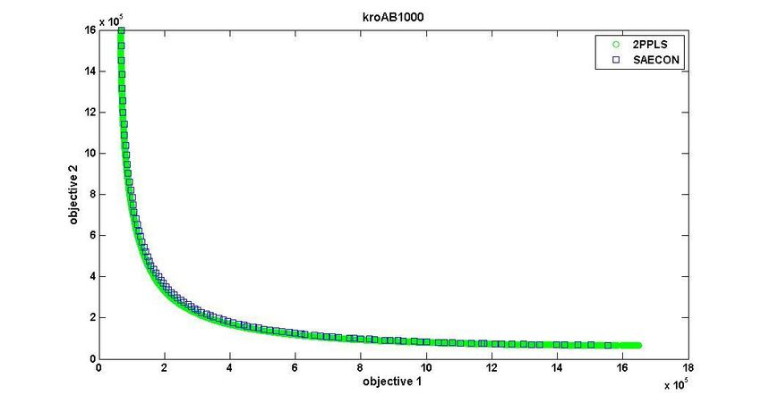
5.2.2 Approximate solution of bi-objective TSP instances with 300 up to 1000 cities
Although the subject of this paper is the exact solution of multi-objective TSP problems, we tried an
approximate method based on ε-constraint for problems with more than 150 cities. For this reason we
developed a variant of Simulated Annealing which solves ε-constraint sub-problems in order to generate
approximately the POS. This approach uses reversal and transport moves as described in [59] (p.366-374)
and also a pre-processing phase with the Lin-Kernighan algorithm of Helsgaun (LKH) [60]. Using this
heuristic approach, we were able to compute good approximations to the problems kroAB300, kroAB500,
kroAB750 and kroAB1000 available in [50].The relevant approximations are shown in Figure 8 for 300
and 1000 city problems. Also, Table 8 reports the convergence [55], hypervolume ratio [54] and spread
[54] metrics for the simulated annealing algorithm vs. 2PPLS. The convergence metric for method „two
phase simulated annealing ε-constraint‟ (2P-SAECON) has been computed for 100 grid points of the ε-
constraint method. Phase one was conducted with the LKH heuristic and 40 grid points for the weights.
Phase two was conducted with ε-constraint/simulated annealing and 100 grid points for the RHS of the
constraint objective 2. As is well known, phase one aims at discovering the supported POS through a
weighted sum approach, and phase two finds the unsupported POS (e.g. in our case with ε-constraint).
By observing Figure 8 and Table 8, we see that the simulated annealing algorithm scales up well with the
problem size and the approximation obtained with 100 grid points for 2P-SAECON is satisfactory in
relation to state-of-the-art 2PPLS. The convergence metric of 2P-SAECON in relation to 2PPLS is of the
order of 10-3 for all problem sizes. The hypervolume ratio is over 0.99 with maximum desired value equal
to 1. Finally, the spread is well below the value of 1, and relatively close to 0 (always well below 0.50)
21which indicates a well distributed Nondominated front. The run time of 2P-SAECON is much shorter
than AUGMECON2-BCHTSP but also significantly larger than the run time of 2PPLS.
(a) kroAB300
(b) kroAB1000
Figure 8. Two phase simulated annealing ε-constraint algorithm (2P-SAECON) compared to 2PPLS approximate
results in BOTSP problems with (a) 300 cities and( b) 1000 cities
22Table 8. Convergence, Hypervolume Ratio and Spread metrics for two phase Simulated Annealing ε-Constraint
(2P-SAECON) with respect to two phase Pareto Local Search (2PPLS) of Lust and Teghem ([13, 6]) in larger scale
datasets of BOTSP with up to 1000 points of interest.
dataset Reference Convergence HV(2p-saecon) Spread(2p-saecon)
Set, R (2p-saecon, R) / HV(R)
kroAB100 3332* 0.0026620 0.992829 0.44071
kroAB300 14867 0.0038793 0.991295 0.37600
kroAB500 33929 0.0040101 0.991519 0.36756
kroAB750 61184 0.0042229 0.991772 0.36412
kroAB1000 98151 0.0042333 0.992035 0.38035
*In kroAB100, R=PF*, and in other larger datasets, R=2PPLS run 1 out of 20.
5.3 Three objective TSP results
Finally, in order to test the AUGMECON2 algorithm in more than two objectives, we constructed a
dataset which we called „3tsp-15‟ with the „portgen‟ generator available in the website
http://dimacs.rutgers.edu/Challenges/TSP/codes.zip with parameter MAXCOORD=1000 and ncities=15
with seeds 1977, 1978 and 1979 for coordinates of objectives 1, 2 and 3, respectively. This is a three
objective TSP problem that was solved with our proposed approach AUGMECON2 using the Miller,
Tucker and Zemlin [61] formulation of the TSP (MTZ). It was solved in 5 hours of CPU providing a
Pareto Front of |PF*|=630 POS which was computed with MS=16886 models solved. This is an exact
solution, which shows that the AUGMECON2 approach can handle three objective TSP problems, but
obviously the number of cities is very small (N=15) in accordance to the literature [62, 63]. Therefore, it
is obvious from these results that in 3-objective problems the number of the Models Solved is much
higher than the number of Pareto Optimal Solutions, especially in relation to the 2-objective cases that we
studied. Conclusively, the generation of the exact Pareto front for 3-objective TSP problems, even of
small size (20-30 cities), is rather an utopian task and the use of approximate algorithms seems to be our
only choice. Our website contains information on the solutions of problems described in Sections 5.2-5.3
as well as on the well-known instances from Section 5.1.
5.4 Two objective SCP results
The AUGMECON2 method was applied to the 44 instances of BOSCP that are described in section 4.2.
The formulation of the problem is the one presented in section 2.2, properly adjusted for the
AUGMECON2 method. The results for the benchmarks with 1 to 11, and types A-D are presented in
Table 9. Where an asterisk (*) is noted, which is the case for 9C, 10C, 10D, 11A, 11B datasets, it means
that 4 threads of CPLEX have been used for the IP sub-problems. Otherwise only one thread of CPLEX
has been used. In their work, Prins et al. [40] present the results for the 4/11 or 16/44 smaller datasets of
Table 9 with up to 40 constraints and 400 variables.
23Table 9. AUGMECON2 performance for BOSCP benchmarks No 1-11.
No File Type # constraints # variables CPU sec |PF*| Models
Solved
1 11 A 10 100 8.64 39 39
B 6.26 43 44
C 2.78 10 11
D 1.45 5 7
2 41 A 40 200 18.01 107 108
B 16.63 108 109
C 7.96 24 25
D 23.87 43 44
3 42 A 40 400 35.83 208 210
B 52.04 276 280
C 31.79 87 91
D 7.14 15 16
4 43 A 40 200 12.80 46 47
B 7.51 28 30
C 3.78 13 14
D 3.48 13 14
5 61 A 60 600 83.66 257 261
B 114.01 338 344
C 18.49 28 31
D 167.29 67 68
6 62 A 60 600 58.10 98 99
B 60.20 99 100
C 211.26 6 7
D 134.17 38 45
7 81 A 80 800 148.66 424 430
B 130.26 354 363
C 7.76 14 17
D 9.33 12 13
8 82 A 80 800 116.51 132 135
B 38.16 88 94
C 671.76 8 9
D 1511.86 44 47
9 101 A 100 1000 375.84 157 270
B 225.50 141 142
C 20933* 13 14
D 3812 24 25
10 102 A 100 1000 104.76 83 87
B 211.48 86 91
C 2464* 14 15
D 16724* 16 23
11 201 A 200 1000 6850* 274 282
B 4278* 282 288
C dnt dnt dnt
D dnt dnt dnt
* 4 threads of CPLEX have been used
24For these smaller datasets, the |PF*| we have found with AUGMECON2 conforms with Prins et al.
results. Furthermore, Lust et al. [38] (p. 265) report that in their work the datasets 201a and 201b
(1000×200) could not be exactly solved. In our paper, we were able to compute the Exact Pareto Set for
201a and 201b in no more than 2hours each. Nevertheless, the 201c and 201d variants (with plateaus at
the objective function coefficients for BOSCP) did not terminate within 24h.
As in the case of the MOTSP we can also observe that the number of models solved is very close to the
cardinality of the Pareto set. This means that AUGMECON2 is very effective in avoiding redundant
iterations that do not result in new POS. This is mainly attributed to the “jumps” caused by the bypass
coefficient b (see section 3.1 and section 3.3) that greatly accelerate the process.
6. Concluding remarks
The aim of this paper is to apply the recently proposed improved version of the augmented ε-constraint
method (AUGMECON2), which is suitable for general MOIP problems, to two popular MOCO
problems, namely, the Multi-Objective Traveling Salesman Problem (MOTSP) and the Multi-Objective
Set Covering Problem (MOSCP). Although AUGMECON2 is designed for the general case, here it is
applied to bi-objective problems confined by benchmark-data availability.
For the MOTSP case the proposed method was a combination of a general purpose MOIP model
(AUGMECON2), with a Branch-and-Cut-and-Heuristic model (BCHTSP) available in GAMS model
library. It was found that the ε-constraint sub-problem is solved almost as many times as the cardinality of
the Exact Pareto Set, which is a very favourable characteristic for a generation approach (no redundant
iterations). Obviously, the BCHTSP model is appropriately modified in order to solve the ε-constraint
sub-problem. Relying on the efficiency of the modified BCHTSP which is used as a subroutine, the
AUGMECON2 method is able to effectively calculate the Exact Pareto Set in 24-60h wall clock time for
every instance of our test bed. A novel feature of our implementation is the parallelization of the
AUGMECON2 loop into indicatively three threads. In general, the AUGMECON2 method is appropriate
for parallelization as the main loop can be divided into independent segments.
In our work it was reaffirmed that MOTSP is among the hardest MOCO problems. Even bi-objective
instances with 100 cities have not been solved exactly in the literature. To the best of our knowledge our
work is the first one that generates the exact Pareto set for 16 popular MOTSP instances with 2 objectives
and 100 cities, studied intensively in the literature. In general, our approach is among the few
implementations able to solve the MOTSP exactly (i.e. produce the exact Pareto set). We also created and
solve exactly a bi-objective problem with 150 cities but probably this is the upper limit for the exact
solution of bi-objective problems with our method and the current hardware. Moving to three objective
functions, the difficulty of generation of the exact Pareto front escalates dramatically and the upper limit
seems to be 15-20 cities, which make the use of exact algorithms prohibitive even for small size multi-
objective TSP problems. We think that a great contribution of our work is that the data sets and the results
are available in https://sites.google.com/site/kflorios/motsp for the interested readers.
Having the exact Pareto set for the BOTSP we were able to assess the effectiveness of state-of-the-art
Multi-Objective Metaheuristics (MOMHs) previously utilized to approximately solve the same 16
datasets. The MOMHs are evaluated, using the two set coverage and convergence metrics exploiting the
information of the Exact Pareto Set. In our case the coverage metric is actually the percentage of POS
25found by the MOMH. The coverage metric in the MOTSP problems varied from 25% to 90% depending
on the type of instances. Euclidean instances were better approximated by MOMH techniques. Random
matrix instances showed poor performance for MOMHs. The mixed type instances yielded
approximations better than random matrix but worse than Euclidean instances, as expected. With respect
to the convergence metric, we found that, in general, state-of-the-art MOMHs approximate very well the
Exact Pareto Set. The magnitude of the convergence metric with respect to the true Pareto Front found by
our work, was either of the order of 10-4 or 10-5, depending on the MOMH type and the instance type.
Another important finding which is in accordance with similar results from other researchers in MOCO, is
that the number of supported POS is only a small proportion among the generated POS. Consequently,
the POS produced using the weighting method (that produces only supported POS) is a remarkable
underestimation of the true Pareto set for the MOTSP.
Regarding the BOSCP, AUGMECON2 succeeded in solving the previously unsolved benchmarks
(instances 201a and 201b) of the MOCOlib for the MOSCP problem. In total, 42 out of 44 benchmarks
were exactly solved, leaving only 2 datasets unsolved (in a 24 hours time limit).
In general, for both kinds of problems, namely MOTSP and MOSCP, the effectiveness of the
AUGMECON2 method is reflected on the fact that for each benchmark the number of model solved is
very close to the cardinality of the Pareto set, indicating good performance and computational economy.
In order to contribute to the testing of relevant algorithms (MOMH or exact algorithms) for the MOTSP
and the MOSCP a web site was created that gathers all the datasets and the results, as well as source code
in Fortran implementing AUGMECON2 and GAMS implementing modified BCHTSP for the ε-
constraint sub-problem.
Extension of our approach, AUGMECON2-BCHTSP to three objective TSPs and massive parallelization
(using more than 3 threads for computations) is studied. The optimal allocation of computational load for
many processors in the bi-objective case is an interesting problem. Also, parallelization of
AUGMECON2 for three objective problems is more delicate, since only the outer loop can be parallelized
safely. Perhaps, the research stream with the most potential for the exact solution of MOTSP is to
substitute the BCHTSP part of the AUGMECON2-BCHTSP algorithm with a fast dedicated exact solver
like CONCORDE [64] or TSP1 [33] but this needs nontrivial programming. The ε-constraint sub-problem
has to be programmed inside CONCORDE or TSP1 which requires effort but would be worthwhile. Also,
comparison of the AUGMECON2 method with other exact schemes for general MOIP problems as well
as the specific MOTSP seems promising (e.g. methods of Lemesre et al. [65] and Dächert et al. [66]).
References
[1] R.E. Steuer, Multiple Criteria Optimization. Theory, Computation and Application, Krieger, Malabar FL,
1986.
[2] C.L. Hwang, A. Masud, Multiple Objective Decision Making. Methods and Applications: A state of the art
survey, Lecture Notes in Economics and Mathematical Systems, 164, Springer-Verlag, Berlin, 1979.
[3] M. Ehrgott, X. Gandibleux, A survey and annotated bibliography of multiobjective combinatorial
optimization, OR Spectrum 22 (2000) 425-460.
[4] C.A. Coello Coello, D.A. Van Veldhuizen, G.A. Lamont, Evolutionary Algorithms for Solving Multi-
Objective Problems, Kluwer Academic Publishers, Boston MA, 2002.
26You can also read