Data-Driven Capability-Based Health Monitoring Method for Automotive Manufacturing
←
→
Page content transcription
If your browser does not render page correctly, please read the page content below
Proceedings of the 6th European Conference of the Prognostics and Health Management Society 2021 - ISBN – 978-1-936263-34-9

       Data-Driven Capability-Based Health Monitoring Method for
                      Automotive Manufacturing
            Alexandre Gaffet1,2 , Pauline Ribot 2,3 , Elodie Chanthery2,4 , Nathalie Barbosa Roa1 and Christophe Merle1

                  1
                      Vitesco Technologies France SAS 44, Avenue du Général de Croutte, F-31100 Toulouse, France
                                                             alexandre.gaffet@vitesco.com
                                                           nathalie.barbosa.roa@vitesco.com
                                                            christophe.merle@vitesco.com

                                  2
                                      CNRS, LAAS, 7 avenue du colonel Roche, F-31400 Toulouse, France
                                                                elodie.chanthery@laas.fr
                                                                  pauline.ribot@laas.fr

                                        3
                                            Univ. de Toulouse, UPS, LAAS, F-31400 Toulouse, France

                                        4
                                            Univ. de Toulouse, INSA, LAAS, F-31400 Toulouse, France

                              A BSTRACT                                        1. I NTRODUCTION
                                                                               In the automotive industry, the large amount of available equip-
Testing equipment is a crucial part of production quality con-
                                                                               ment data promotes the development of data-driven methods
trol in the automotive industry. For those equipments a data-
                                                                               when designing health monitoring systems. If complete in-
based Health Monitoring System could be a solution in order
                                                                               formation about the equipment health status and its mainte-
to avoid quality issues and false alarms, that reduce produc-
                                                                               nance operations is available, supervised methods are pre-
tion efficiency, potentially leading to huge losses. In man-
                                                                               ferred. Conversely, if the information is uncertain or unavail-
ufacturing industries, a widely accepted index for evaluat-
                                                                               able, unsupervised methods should be considered. Unsuper-
ing process performance is the process capability, which as-
                                                                               vised methods are often based on statistical models that learn
sumes data following a normal distribution. In this article we
                                                                               trends or anomalies in the data.
propose a capability-based health monitoring method based
on electrical test data. These data might vary according to                    One major challenge of the monitoring is to find the appropri-
the testing equipment, but also on manufacturing parameters.                   ate health indicator for the problem. An approach could be to
Gaussian Mixture Models (GMM) are used to model the data                       use a known health indicator with some interesting properties
distribution exposed to equipment and parameter variations                     linked to the problem under study. For instance, (Baraldi,
supposing that the hypothesis of normal distribution of the                    Di Maio, Rigamonti, Zio, & Seraoui, 2015) used spectral
data holds. Two approaches are discussed for selecting the                     residual as input of an unsupervised algorithm. Another ap-
GMM number of modeled distributions. The first approach                        proach is to learn it using artificial neural networks (Ren et
is based on the well-known Bayesian Information Criterion                      al., 2019).
(BIC). The second approach uses a new multi-criteria index
                                                                               In industry, Statistical Process Control (SPC) is a common
function. The health monitoring method is evaluated on real
                                                                               approach to achieve a good quality of production. Links be-
data from In-Circuit Testing (ICT) machines for electronic
                                                                               tween the actual performance of production and specification
components at a Vitesco factory in France.
                                                                               limits are made using capability indexes (Wu, Pearn, & Kotz,
                                                                               2009). With these indexes the health monitoring is based
                                                                               on the probability of finding out-of-bounds outputs from a
                                                                               process. Nonetheless, process capability indexes are usually
Alexandre Gaffet et al. This is an open-access article distributed under the   used to supervise the production and do not distinguish the
terms of the Creative Commons Attribution 3.0 United States License, which     source of anomalies. Possible sources are the equipment, the
permits unrestricted use, distribution, and reproduction in any medium, pro-
vided the original author and source are credited.                             product or its components. The goal of this article is to use

                                                                                                                                            1

                                                                         Page 172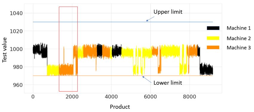
E UROPEAN
Proceedings of the C ONFERENCE
6th European ConferenceOF
of the P ROGNOSTICS
THEPrognostics AND HManagement
and Health EALTH M ANAGEMENT S OCIETY
Society 2021 - ISBN 2021
– 978-1-936263-34-9
such capability indexes for health monitoring purposes and sion. A PCB contains several components of different forms
isolate the cause of an anomaly. To this end, the use of Gaus- and sizes. The amount of components varies from 10 to 1000,
sian Mixture Models (GMM) is proposed. Mixture modeling however, each component needs to be tested individually. For
is a powerful statistical technique for unsupervised density that purpose one or more test steps are required. The usage of
estimation, especially for high-dimensional data (Mehrjou, test versions allows to track any changes on the test steps and
Hosseini, & Araabi, 2016). parameters. This product specific approach entails a tremen-
dous amount of combinations to analyse, accordingly, the
The GMM method requires the selection of a number of mix-
chosen monitoring methodology must easily adapt to prod-
ture components, a fitting algorithm and an initialisation method.
uct references and test versions.
To select the right number of mixture components at least two
approaches are possible: the Maximum A Posteriori (MAP) The study uses two years of historical data from ICT equip-
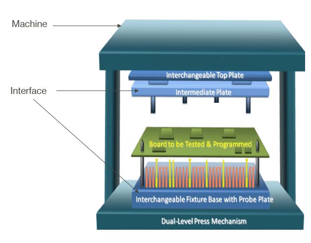
approach and the full Bayesian approach. The MAP approach ment for several products. As illustrated in Figure 1, on the
selects the most likely hypothesis according to the data and a ICT two elements interact to make the process product spe-
prior distribution of the parameters and is often more tractable cific. The first element is the ICT machine, which analyses
than full Bayesian learning (Montesinos-López et al., 2020). the results. All machines can be used for all product families.
For the MAP approach, two criteria are presented: the Bayesian The second element is the interface composed of a pneumatic
Information Criteria (BIC) and a Mixed-criteria method cre- bed-of-nails wired to fit the specific design of each product
ated by machine learning. In this work the Expected Max- family and to test its electronic components.
imisation (EM) algorithm is chosen as a fitting algorithm for
Data coming from one interface, one test, one test version and
GMM. Different initialisation methods are compared on real
multiple machines can be seen as a time series. These time
data in order to select the most appropriate method for the
series will be truncated since the production of one specific
application.
product and test version is often discontinuous. Furthermore,
In the considered industrial use case the tested products corre- in the meanwhile the same machine can be used for testing
spond to Printed Circuit Boards (PCB) where electronic com- other products with other interfaces. It is then impossible to
ponents are placed using Surface Mount Technology (SMT). extract a continuous time series from test data, which repre-
These components are then tested by In Circuit Testing (ICT) sent one of the main challenges of this dataset.
machines. Because of the uncertainty on the completeness
of maintenance data, this paper proposes an original unsuper-
vised health monitoring method using capability index as a
health indicator. It uses tests values to detect faults linked to
the equipment or with the products. The main contribution of
the work is to show that these kinds of methods can provide
useful knowledge for equipment health monitoring.
This paper is organized as follows. Section 2 is devoted to the
presentation of the dataset and our capability-based method-
ology. Section 3 presents the MAP approach and the two
proposed criteria to find the best number of mixture compo-
nents. Section 4 discusses three different initialisation strate-
gies. Application of the capability based methodology is pro-
vided in Section 5. Conclusions and future work are finally
presented in Section 6. Figure 1. ICT equipment
2. M ETHODOLOGY Another challenge in the dataset is the large number of fea-
tures. For each reference of product there are around 1000
2.1. Industrial database tests. The developed a solution should be valid for all these
Vitesco production is grouped into product families, accord- tests, therefore, have a large power of generalization. Since
ing to their design and application. Within each of these ICT tests are supposed to follow a normal distribution, the use
product families several product references can be found. For of a process capability index, defined in Section 2.2, seems to
the sake of standardisation, the production of electronic cards be adapted to evaluate the test process and the health of the
uses substrates of similar size for each family. This substrate testing equipment. For each test in our dataset the parameters
is called a panel. Panels are composed of identical dupli- are the ICT machine, the interface and the product position.
cates of the same product. Electrical tests are designed for All of these parameters are equipment related. Nonetheless,
individual product references and have an associated test ver- there are also product-related parameters. Indeed, for each
product, the mounted electronic components, i.e. the raw ma-
2
Page 173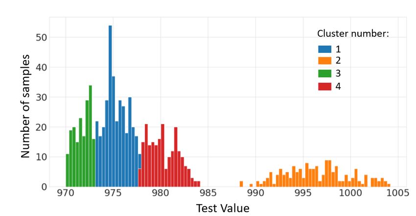
E UROPEAN
   Proceedings of the          C ONFERENCE
                      6th European ConferenceOF
                                             of the P ROGNOSTICS
                                                THEPrognostics     AND HManagement
                                                               and Health EALTH M ANAGEMENT   S OCIETY
                                                                                    Society 2021 - ISBN 2021
                                                                                                        – 978-1-936263-34-9

terials, might come from different providers or have different      2.3. Overview of the methodology
values within the expected tolerance. These sources of vari-
                                                                    The proposed methodology is described in Figure 2. The in-
ability cannot be controlled in the manufacturing process. For
                                                                    coming time series is defined by selecting one test version,
example, the temperature of the oven may be different and
                                                                    one test, one period and one interface for that test version.
have an influence on the distribution of the component val-
                                                                    Production periods are defined for one interface as the time
ues. The idea is then to create groups of products that have the
                                                                    between two machine replacements. The method starts with a
same parameters. In theory, splitting the data set by machine,
                                                                    clustering stage during which Gaussian distributions are iden-
interface and test will result in a normal distribution for each
                                                                    tified in the input data. To each identified mixture component
split. However, this neglects the influence of the raw mate-
                                                                    corresponds a cluster. Then, for each of these mixture compo-
rials and the manufacturing process. Nonetheless, including
                                                                    nents, a criticality index is computed as well as a cluster con-
this information is difficult because the number of parame-
                                                                    fidence index. This index is called the Posterior Uncertainty
ters to define each group is significantly large. The idea is to
                                                                    Index (PUI) in the following sections. Then, a detection stage
group the data samples according to the distribution created
                                                                    compares both indexes to thresholds to decide whether the in-
by the unconsidered parameters. In fact, multiple sets of pa-
                                                                    put triggers an alarm or not. When an alarm is triggered, its
rameters could lead to the same distribution. Henceforward,
                                                                    root cause analyse starts.
the hypothesis of normality for these distributions is made.
                                                                    To identify Gaussian models, the method starts by fitting a
2.2. Capability                                                     GMM that clusters the input data. A MAP approach is used
                                                                    to determine the best number of components in the mixture.
We propose a methodology based on process capability which
                                                                    There are no constraints on the variances and means of GMM.
is a well-known index in the industry. This index is calcu-
                                                                    A particular initialisation strategy is chosen and argued in
lated over a sample of data given an upper limit and a lower
                                                                    Section 4. The clustering stage takes as input a time series
limit. These limits are defined by an expert during the design
                                                                    defined as one period of one test and returns as output the
and pre-industrialisation stages of the product. Under some
                                                                    mixture components identified in the period. The clusters
normality conditions, the index is directly proportional to the
                                                                    correspond to the different Gaussian distributions identified
probability that a point in the sample is greater than the up-
                                                                    in the time series.
per limit or lower than the lower limit. There are different
capability indexes depending on the controlled process. We          In order to obtain an index with highly generalizing prop-
decide to use the CP k process capability index.                    erties related to the health state of the equipment, the CP k
                                                                    index has been chosen as the criticality index. One of the ad-
The choice of this particular capability index among all pos-
                                                                    vantages of GMM is to build cluster membership functions
sible capability indexes is guided by the application and the
                                                                    for all points. These functions are used to propose an index
dataset. In machine tool capability (CP ), the size of the de-
                                                                    of the quality of the mixture. The objective of this second in-
viations from the average value of the process determines
                                                                    dex, the PUI index, is to control the posterior uncertainty of
the location of the process within the specified limit. Nev-
                                                                    the chosen mixture components of all GMM points.
ertheless, as in our case the process is not always centred
between the specification limits, the CP k index is a better        During the detection stage, the CP k and the PUI indexes are
index. Two other capability indexes could also be interesting:      used. The CP k index is compared to a threshold fixed as a
CP m, so-called Taguchi index (Hsiang, 1985) and CP mk,             model parameter. It determines the criticality of the input data
which combines the CP m and CP k indexes (Boyles, 1991).            cluster. Indeed, the smaller the CP k, the higher the proba-
The Taguchi index measures the ability of a process to re-          bility of encountering out-of-bounds tests. The PUI is also
turn values around a target value. We decide not to use these       compared to a threshold to determine if the built mixture is
indexes because they require the target value of the compo-         acceptable. If mixture is not acceptable, all test values in the
nents which in our case does not change in time, contrary to        period are assigned to the same cluster and CP k is recom-
the specification limits. The CP k index is defined as follows:     puted with it. The goal of this health monitoring stage is to
                                                                  detect within the acceptable mixtures those input clusters that
                            U L − µ(X) µ(X) − LL                    have a high probability of containing out-of-bounds test val-
       CP k(X) = min                    ,                   (1)
                              3σ(X)         3σ(X)                   ues.
with X a sample of points, µ, σ, U L, LL the mean, the stan-        If the input clusters have out-of-bounds CP k index and PUI,
dard deviation, the upper limit and the lower limit, respec-        then an isolation stage starts. These clusters are then called
tively.                                                             critical clusters. The idea is to compare the criticality index
                                                                    between ICT machines, interfaces and product positions in
                                                                    order to isolate the detected fault. In our case, the isolation
                                                                    consists in finding the elements responsible for the critical

                                                                                                                                  3

                                                              Page 174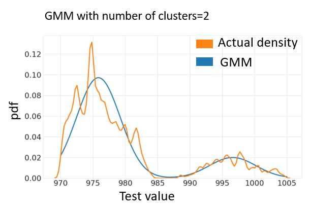
E UROPEAN
   Proceedings of the          C ONFERENCE
                      6th European ConferenceOF
                                             of the P ROGNOSTICS
                                                THEPrognostics     AND HManagement
                                                               and Health EALTH M ANAGEMENT   S OCIETY
                                                                                    Society 2021 - ISBN 2021
                                                                                                        – 978-1-936263-34-9

                                             Figure 2. Overview of the proposed method

clusters. Possible candidates are the ICT machine, the inter-         with n the number of points of one period.
face and the product group.
                                                                      Nonetheless, like k-means, the EM algorithm gives a local
                                                                      optimum solution. This means that the solution depends on
2.4. Gaussian Mixture Model
                                                                      the initialisation of the algorithm. The quality of the solu-
Our methodology requires an unsupervised machine learning             tion relies on the chosen initialisation strategy. Initialisation
algorithm to automatically identify the distributions in a time       strategies are discussed in Section 4.
series defined for one test and one period. For our data, the
hypothesis of normality is considered, i.e. the distributions to      3. M ODEL SELECTION STRATEGIES
be identified are Gaussian distributions.
                                                                      In order to choose the best number of distributions to con-
Among the iterative clustering algorithms, k-means is one of          sider during the GMM stages, two solutions are investigated.
the most popular. However, in our case, its application is diffi-     The first solution is linked to the popular Bayesian Informa-
cult because the variance for each distribution can be different      tion Criterion (BIC) (Schwarz et al., 1978) and Akaike In-
and k-means can be seen as a GMM with spherical Gaussian              formation Criterion (AIC) (Akaike, 1998). To determine the
functions having a common width parameter σ (Bishop et al.,           best number of distributions, this solution considers the prob-
1995).                                                                lem as a component density estimation problem. It searches
                                                                      for a mixture solution that has a Probability Density Func-
The Expected Maximisation (EM) algorithm for the GMM
                                                                      tion (pdf) as close as possible to the pdf of the data. If the
method seems to be more appropriate for the data. The EM
                                                                      hypothesis of normality of data is respected, the considered
algorithm iteratively improves an initial clustering solution in
                                                                      approximation is adequate according to the properties of the
order to better fit the data to the chosen mixture (McLachlan
                                                                      BIC explained in Section 3.1. The second solution considers
& Thriyambakam, 1997). The solution is the locally optimal
                                                                      a trade-off between the BIC and some properties of the mix-
point with respect to a clustering criterion. The criterion used
                                                                      ture components and the distributions formed by the GMM.
in the EM algorithm is the log-likelihood. It represents the
                                                                      These properties are: the skewness and kurtosis of the mix-
probabilistic measure of how well the data of the EM algo-
                                                                      ture components and the overlap of the distributions. We pro-
rithm fit the mixture. Another advantage of the EM algorithm
                                                                      pose a Mixed-criteria method to determine the best number
compared to k-means concerns the membership function of
                                                                      of mixture components for the GMM.
the identified clusters. Indeed, k-means uses a membership
function that assigns a point to a single cluster. Therefore, it is
                                                                      3.1. Model order selection : BIC
not possible to describe the uncertainty of clustering for each
point. On the contrary, for GMM, the membership functions             Determining the correct number of mixture components in an
can take any value between 0 and 1 and can be used to build           unsupervised learning problem is a difficult task. For GMM
an uncertainty index (Bradley, Fayyad, & Reina, 1999). Let            the problem can be translated into finding the right number
µk (x) denote the membership function of the cluster k ∈ K            K of normal distributions in the mixture. A finite mixture
for a point x with K the number of mixture components of              distribution G is defined as:
the GMM. Posterior Uncertainty Index (PUI) is defined by                                         K
                                                                                                 X
                            n
                            X                                                              G=          ηk fk (y|θk )               (3)
                   PUI =          max(µk (xi ))                (2)                               k=1
                                  k∈K
                            i=1

                                                                                                                                     4

                                                                Page 175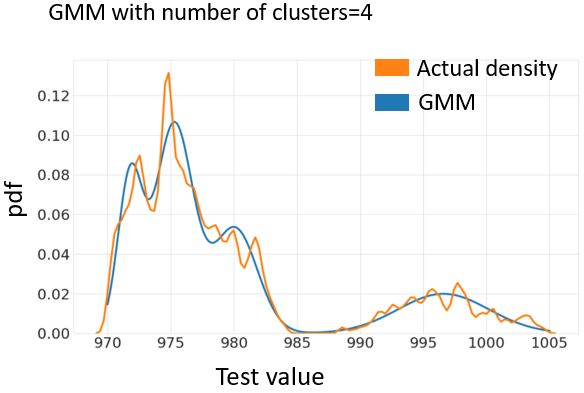
E UROPEAN
   Proceedings of the          C ONFERENCE
                      6th European ConferenceOF
                                             of the P ROGNOSTICS
                                                THEPrognostics     AND HManagement
                                                               and Health EALTH M ANAGEMENT   S OCIETY
                                                                                    Society 2021 - ISBN 2021
                                                                                                        – 978-1-936263-34-9

where ηk are the weights of the k th GMM normal distribu-            3.2. Model based clustering : Mixed-criteria method
tion, fk is its density function parametrised by θk and y =
                                                                     As AIC and BIC have different, interesting properties, some
(y1 , ..., yn ) are the observations, i.e. the data in one period.
                                                                     articles try to combine them. (Barron, Yang, & Yu, 1994)
Selecting a wrong K may produce a poor density estimation.           proposed the creation of a criterion that combines both of
A common approach to select the best number of features              them into a single one, while (Hansen & Yu, 1999) proposed
is the MAP approach. This approach creates mixtures with             to switch between these criteria using a statistical parameter.
different numbers of distributions. Depending on a criterion,        More recently, (Peng, Zhang, Kou, & Shi, 2012) proposed a
the approach will select the best mixture model. The most            multiple criteria decision-making based approach using valid-
popular criteria for model selection are BIC and AIC. These          ity indexes for crisp clustering. We propose a method that can
criteria are based on the log likelihood function of a mixture       mix BIC with other criteria, combining their strengths to ob-
model MK with K being the number of mixture components.              tain clusters better suited to our problem than those obtained
Let n be the number of points of the dataset, the log likelihood     with a single criterion. To improve the completeness of the
is defined as:                                                       method, a dataset with similar properties to the one of this
                                                                     study is created. The learning of the criteria aggregation is
                 l(θK ; K) = log(L(θK ; K))                   (4)    done with that dataset. This subsection describes our propo-
with                                                                 sition for the chosen criteria and the aggregation function.
                             n X
                             Y   K
              L(θK ; K) =      [   ηk fk (yi |θk )].          (5)    3.2.1. Chosen criteria
                             i=1 k=1
                                                                     Several criteria are chosen as input parameters. In addition to
Both BIC and AIC use the penalty term vK defined as vK =             the inference-based criteria BIC and AIC mentioned before,
K(1 + r + r(r + 1)/2) − 1 with r the number of features in           we also considered the Normalized Entropy Criteria (NEC)
the dataset. This penalty term is proportional to the number         introduced by (Celeux & Soromenho, 1996) and defined as:
of free parameters in the mixture model Mk and penalises the
complexity of the model. BIC is defined as follows:                                                      E(K)
                                                                                   N EC(K) =                                      (8)
                                                                                                  l(θK ; K) − l(θ1 ; 1)
            BIC(K) = −2l(θK ; K) + vK log(n)                  (6)
                                                                     where E(K) is an entropy measure which involves the pos-
with n the number of points.                                         terior probabilities of yi belonging to the k th mixture com-
AIC is defined as follows:                                           ponent. Entropy measure is computed by the following equa-
                                                                     tion:
                                                                                                  XK X n
               AIC(K) = −2l(θK ; K) + 2vK                     (7)
                                                                                     E(K) = −            tik ln(tik )           (9)
                                                                                                  k=1 i=1
BIC approximates the marginal likelihood of a mixture model
                                                                     with
Mk and AIC is related to the Kullback-Leibler divergence be-                                   ηk fk (yi |θk )
tween the mixture model and the real dataset. Both criteria                            tik = PK                                  (10)
have, under appropriate regular conditions, interesting prop-                                 j=1 (ηj fj (yi |θj )

erties. In particular, they both assume that the true distribu-      and l(θK ; K), l(θ1 ; 1) the log likelihoods as defined in Equa-
tion of the data lies within the created mixture models. Under       tion (4). By definition, N EC(1) = 1.
this condition, BIC has been shown to be consistent (Yang,
                                                                     NEC is linked to the overlap between the normal distribu-
2005). Indeed, if among the created mixture models, a model
                                                                     tions of the studied mixture. AIC, BIC and NEC can take
has the distribution of the data, it will be selected by BIC. For
                                                                     very different values depending on the dataset. That is why it
AIC, it has been shown that it is minimax optimal, i.e. it will
                                                                     is mandatory to normalise them in order to use them for ma-
select the model that minimises the maximum risk among all
                                                                     chine learning. A min-max normalisation is chosen, so that
the built models (Yang, 2005). However, these regular con-
                                                                     each new criterion will take a value between 0 and 1. The
ditions are often not met in practice. In particular for BIC,
                                                                     normalisation procedure is described as follows: Let Fe,k be
Laplace approximations are often invalidated. Nevertheless,
                                                                     the value of the input feature for the experiment e and clus-
in practice the consistent property of BIC seems to still be
                                                                     ter number k. Let N ormFe,k be its normalised value, it is
present if the objective of the mixture is to estimate density
                                                                     defined as:
(Fraley & Raftery, 2002), (Roeder & Wasserman, 1997). On                               (
the contrary, if the objective is to estimate the real number of                           − minp∈[1:P ] (Fe,p )+Fe,k
                                                                                                                      if θ(e) 6= 0
mixture components, AIC is known to overestimate this value             N ormFe,k =                  θ(e)
                                                                                           0                          else
(Celeux & Soromenho, 1996). Therefore, we choose to use                                                                           (11)
BIC as the first method for our application case.

                                                                                                                                    5

                                                               Page 176
E UROPEAN
Proceedings of the C ONFERENCE
6th European ConferenceOF
of the P ROGNOSTICS
THEPrognostics AND HManagement
and Health EALTH M ANAGEMENT S OCIETY
Society 2021 - ISBN 2021
– 978-1-936263-34-9
with computed and the GMM with the maximum probability for
the selected period j and number of distributions k in [1 : P ]
is chosen as GM Mj,K∗
.
θ(e) = − max (Fe,p ) + min (Fe,p ) (12)
p∈[1:P ] p∈[1:P ]
Algorithm 1 Best Model Selection
Other criteria linked to the normality of the clusters created
by K mixture components are also considered: 1: Input:
2: Dataset with J periods
3: P , number of distributions to test
4: Random forest classifier already fitted
M kj = max (|kurtosisk,j |) (13) 5: Empty list of GMM
k∈[1,K] 6: Dataset with J periods
k=K 7:
X
mkj = (|kurtosisk,j |) (14) 8: Output:
9: List of GM M ∗
k=1
10:
M sj = max (|skewnessk,j |) (15) 11: for j in 1, ..., J do
k∈[1:K]
12: M axproba = 0
k=K
X 13: for k in 1, ..., P do
msj = (|skewnessk,j |) (16) 14: Fit GMM with period j and k number of distribu-
k=1 tions GM Mj,k
15: Compute Xj,k
mediank,j
M mj = max |1 − | (17) 16: Compute α(Xj,k ) using Random forest classi-
k∈[1,K] meank,j fier
X
k=K 17: if α(Xj,k ) > M axproba then
mediank,j 18: GM Mj,K ∗
= GM Mj,k
mmj = |1 − | (18)
meank,j 19: M axproba = α(Xj,k )
k=1
20: Insert GM Mj,K ∗
in list of GM M ∗
In these equations, the index k, j implies that the selected
value is calculated on the k th distribution of the mixture for
In order to assess the performance of the models selected as
the period j.
best for each criteria (GM M ∗ ), an evaluation metric m is
For clarity, the set of normalised BIC, AIC, NEC and normality- defined. This metric is computed for each dataset sample s
linked criteria is henceforth called Xj,K . and each criterion Xj,K as follows:
3.2.2. Aggregation function and performance assessment
of the criteria 1 if the criterion Xj,K finds the right number of
ms,Xj,K = mixture components for sample s
The aggregation function is based on the results of a cluster-
0 else.
ing stage. This article uses the random forest classifier as it
outperforms support vector machines and logistic regression
for our application. The algorithm classifies the GMMs with 3.3. Synthetic database
the right number of mixture components into the class “rec- In order to compare the results of the model selection with the
ognized” and the others into the class “not recognized” using two approaches described in the sections 3.1 and 3.2, some
the chosen criteria Xj,K as input. Nevertheless, this clus- 1D synthetic databases composed of several normal distribu-
tering has a major drawback: for one period, several GMMs tions are created. For the database generation, the procedure
can be classified in the “recognized class”. Instead of using given by (Qiu & Joe, 2006a) is adapted. The general idea is
these classes directly, the aggregation function uses the poste- to create several datasets based on an experimental design. In
rior probability of the “recognized” class defined as α(Xj,K ). order to generate a balanced database, four factors are used:
This allows to choose the best model among the models clas-
sified in the recognized class. The selected model is the one 1. The number of clusters for one example,
with the maximum posterior probability. 2. The minimum separation degree,
The pseudo-algorithm for the aggregation function is described 3. The relative cluster density,
in Algorithm 1. First, for each period in [1 : J], GMMs are
fitted with a number of distributions ranging from 1 to P . 4. The sample size.
Next, the chosen criteria Xj,k required by the random forest For the first factor, values [1, 2, 3, 4, 5] are used to match the
classifier are computed for each GMM. Then, the posterior tests to the exploratory analysis conducted on the industrial
probability α(Xj,k ) given by the random forest classifier is dataset.
6
Page 177E UROPEAN
Proceedings of the C ONFERENCE
6th European ConferenceOF
of the P ROGNOSTICS
THEPrognostics AND HManagement
and Health EALTH M ANAGEMENT S OCIETY
Society 2021 - ISBN 2021
– 978-1-936263-34-9
Table 1. Factors of the design of experiments Table 2. Performance comparison of criteria
Factor Values Criterion Generated Distributions
Number of clusters {1, 2, 3, 4, 5} All 1 2 3 4 5
AIC 0,684 0,808 0,752 0,665 0,640 0,561
Minimum separation degree {10−5 , 0.01, 0.21, 0.34} BIC 0,986 0,989 0.995 0,989 0.993 0,965
Relative cluster density {all equal, one cluster 10% NEC 0,926 0,872 0,992 0,936 0,908 0,921
of data, one cluster 60% of mk 0,524 0,975 0,890 0,363 0,226 0,175
data} Mk 0,664 0,955 0,884 0,534 0,471 0,478
Sample size {500, 1000, 2000} Ms 0,423 0,994 0,661 0,273 0,135 0,056
ms 0,339 0,994 0,554 0,138 0,006 0,003
mm 0,264 0,978 0,179 0,064 0,074 0,021
The minimum separation degree is defined in (Qiu & Joe, Mm 0,227 0,895 0,115 0,050 0,049 0,019
Mixed-criteria 0,993 0,997 0,997 1,000 0,995 0,997
2006b) as an index extracted from an optimal dimension pro-
jection. In our case, the degree is simplified as follows:
Lk (a) − Uk0 (a) much better than AIC. The Mixed-criteria method improves
Z(a) = (19) the results of the BIC criterion and almost always finds the
Lk0 (a) − Uk (a)
right number of mixture components.
with Lk , Uk , Lk0 and Uk0 the lower and upper a
2 percentiles
of classes k and k 0 . In our case, both BIC and Mixed-criteria method can be used.
The main differences in the clusters obtained with both ap-
(Qiu & Joe, 2006b) present three separation values for the proaches are found for the overlap cases. The Mixed-criteria
generation: Z = 0.01 indicates a close structure, Z = 0.21 method is less likely to accept mixtures with overlapping be-
indicates a separated structure and Z = 0.34 indicates a well- tween distributions, while this does not directly affect BIC.
separated cluster structure. We choose to add the value Z =
10−5 to create a very closer structure because in our data, we 4. I NITIALISATION STRATEGIES
have closer structure than the ones created with Z = 0.01.
Initialisation strategies are very important to limit cost time
The relative cluster density factor is based on (Shireman, Stein- of an algorithm. As the method has to be run at least 1000
ley, & Brusco, 2017) and is defined as follows: times per product, the cost time is an important parameter.
1. all clusters have the same number of points, For our application, the choice is made to test three different
categories of initialisation strategies.
2. one cluster has 10% observations and the other clusters
have the same number of observations,
4.1. Random initialisation
3. one cluster has 60% of the observations and the other
clusters have the same number of observations. Initialisation strategies based on stochastic methods are quite
popular. Among them, two methods are tested. A first basic
Finally, the considered sample size values are [500, 1000, 2000]. strategy consists in initialising the EM input parameters ran-
This corresponds to the period length in the application. Ta- domly for a fixed number of Gaussian distributions. The EM
ble 1 summarized the factors used in the proposed design of parameters are in that case the variance, the mean, and the
experiment. weight of each mixture component.
3.4. Results (Biernacki, Celeux, & Govaert, 2003) presents the second
strategy called “emEM” (for expected maximisation Expected
Model selection results are obtained by a cross-validation over Maximisation). This method starts with a stage called short
the test data. The dataset is divided into four random parts in- EM. In this stage, an EM algorithm is run for several itera-
dexed by t in the following. Then, each part of the dataset tions from random starting points. The number of iterations
is chosen as the test dataset, the three other parts are used to of this stage is set as a parameter. Finally, among the solutions
learn the random classifier inside the Mixed-criteria method. given by the short EM, the strategy with the highest likelihood
The results presented in Table 2 correspond to the following is chosen. Then the EM algorithm is run, starting with the pa-
evaluation metric D: rameters of the chosen solution. This allows more initialisa-
4 X
X S tion solutions to be explored or less time to be spent exploring
1
D= · ms ,i (20) the same number of initialisation solutions. This approach,
4 · S t=1 s =1 t
t which is considered the most efficient by (Biernacki et al.,
2003), has some drawbacks. The maximum number of itera-
with S the number of samples per parts. The closer D is to 1,
tions in the short EM stage has to be defined by the user and
the better the model selection.
can have a huge impact on the final result of the algorithm.
The results in Table 2 show that BIC is very good at deter- Moreover, this parameter can change depending on the con-
mining the right number of mixture components and works sidered test and period. Another drawback, shared by both
7
Page 178E UROPEAN
Proceedings of the C ONFERENCE
6th European ConferenceOF
of the P ROGNOSTICS
THEPrognostics AND HManagement
and Health EALTH M ANAGEMENT S OCIETY
Society 2021 - ISBN 2021
– 978-1-936263-34-9
approaches, is that they can lead to locally optimal solutions the computation time of the evaluated strategy.
when too few initialisations are performed. This drawback is
aggravated for the emEM because the first stage restricts the 4.4.1. Best global solution
search space by construction.
The best global solution is given by BIC. The lowest BIC is
the best local solution that can be given by the EM algorithm
4.2. K-means initialisation
in terms of fitting the Gaussian mixture density. Therefore,
Some methods use the results of a k-means clustering al- this criterion is chosen as an indicator of the fitting algorithm.
gorithm as input of the EM algorithm. In (Steinley & Br- For each input, the l strategy with the lowest BIC receives a
usco, 2011), a theoretical property between the parameters score ζj,l equal to 1 and the other strategies receive a score
extracted from a solution given by a k-means algorithm and of 0. Then, for each initialisation strategy l, a global index
a mixture model is demonstrated. The main drawback of this called GF Il (Global Fitting Index) is built over all inputs and
approach is that, as for random methods, it could lead to lo- is defined as follows:
cally optimal solutions. Additionally, the number of initiali- J
sations of the k-means procedure is also a parameter to settle. 1X
GF Il = ζj,l (21)
Another drawback relates to the solutions generated by this J j=1
method. When clusters overlap, k-means has difficulties in
representing correctly the data. Moreover, when the data have with
a large difference in variance within their Gaussian distribu-
1 if BICj,l = maxi∈[1,L] (BICj,i )
tion, k-means is not the most suitable algorithm (Shireman et ζj,l = (22)
0 else.
al., 2017).
where J is the number of inputs, l is the evaluated strategy, L
A classical procedure with a fixed number of initialisations
is the total number of strategies evaluated and j indexes over
of the k-means method has been tested. It gives a set of so-
all inputs.
lutions which are then used as input for the EM algorithm.
In addition, an approach with “short EM”, similar to the one
4.4.2. Distance to the optimal solution
with the random initialisation method, has also been tested.
One of the main drawbacks of the previous metric is that if an
4.3. Otsu initialisation initialisation strategy is always the second best, it will have a
GF I of 0, even if it could be an acceptable solution. In order
One of our contributions is a new initialisation strategy adapted
to complete the evaluation, another metric ∆ is proposed and
to small dimensions. It is based on a clustering procedure,
defined as follows:
named the Otsu method. This method, described in (Otsu,
1979), is widely used for image segmentation. The initial ob- J
X
jective of the method is to select thresholds between levels in ∆l = scorej,l (23)
a greyscale image. It is based on the 1D histogram of grey j=1
levels. For a foreground/background problem, the selected with
threshold is defined as the one that minimises the intra-cluster Distopt (j, l) if βj 6= 0
variance. This problem can be translated as finding different scorej,l = (24)
0 else.
distributions in a greyscale histogram, which has similarities
with our clustering problem. For multiple clusters, an im- mint∈L (BICj,t ) − BICj,l
plementation of this algorithm is described in (Liao, Chen, Distopt (j, l) = (25)
βj
Chung, et al., 2001). For our application, the outputs of the
multi-cluster Otsu method are used as input by the EM al- and
gorithm. One of the main drawbacks of this approach is the βj = (max(BICj,t ) − min(BICj,t )) (26)
t∈L t∈L
restriction of the search space to only one possible result.
with l a strategy of initialisation and j one period.
4.4. Evaluation of the initialisation strategies
4.4.3. Time and Parameters
The following procedure is used in order to evaluate the qual-
In order to evaluate the efficiency of each initialisation strat-
ity of performance of different initialisation methods. The in-
egy, the elapsed time required by the EM algorithm and the
put is a dataset divided into samples. One sample represents
initialisation is measured. The time was measured from the
a period of production of one test. The performance of each
beginning of the initialisation for the first test to the end of
initialisation method is evaluated according to three criteria:
the clustering for the last test of the database. Then, the mean
the ability to find the best global solution (BIC in our case),
elapsed time per period for each set of parameters and each
the ability to find the closest result to the optimal solution and
8
Page 179E UROPEAN
Proceedings of the C ONFERENCE
6th European ConferenceOF
of the P ROGNOSTICS
THEPrognostics AND HManagement
and Health EALTH M ANAGEMENT S OCIETY
Society 2021 - ISBN 2021
– 978-1-936263-34-9
initialisation method is computed.
In order to assess the performance of an initialisation method,
a design of experiments is proposed. Four factors are used:
1. The initialisation method: k-means, Random or Otsu;
2. The convergence threshold;
3. The number of iterations of the short EM part of the al-
gorithm;
4. The number of initialisations.
For the Otsu initialisation method, the only possible factor is
the convergence threshold. When the convergence threshold
is less than the lower bound gain on the likelihood, the EM it- Figure 4. Best global solution vs mean time per period for
erations stop. The convergence threshold tested values are k-means initialisation method solutions
[10−5 , 10−4 , 10−3 , 10−2 ]. The tested number of iterations
of the short EM part are [10, 20, 50, 100, 200, inf ], when the
number is infinite, then there is no short EM stage. The tested
values of the number of initialisation are [10, 20, 40, 50, 60].
The presented results are obtained with 100 tests and 14 peri-
ods for each test.
Figure 5. Distance to the optimal solution vs mean time per
period for k-means initialisation method solutions
5. A PPLICATION OF THE PROPOSED METHOD FOR ONE
TEST VERSION
Figure 3. Best global solution vs mean time per period The method described in Section 2.3 was implemented on a
dataset formed by the test values for one test version and for
By analysing the results presented in Figure 3, it can be ob- two interfaces. The method was implemented with Python 3.
served that the k-means method has globally the best solu- The EM algorithm and Random Forest are from the scikit-
tions in terms of GF I. In the meanwhile, the solutions pro- learn library. The studied version has 1012 tests per product.
vided by the random initialisation method are faster than those In order to choose the thresholds of the CP k index and of
obtained with k-means but provide less fitted solutions. The the PUI, a directory of maintenance operations is used. Three
Otsu initialisation method has a GF I score close to that of tests lead to maintenance operations. The value of threshold
k-means only for the smallest convergence threshold. Fur- 1 for the CP k index and 0.8 for PUI allow the detection of
thermore, the initialisation time of the Otsu method seems to these three tests found in the maintenance operation direc-
be too large to be competitive against the k-means method. tory. Moreover, the method also detects ten other tests whose
For these reasons, the k-means initialisation method is cho- distributions are in contradiction with the specification lim-
sen in the following part and the different scores are then re- its previously defined as U L and LL in Equation 1. This
computed for the solutions given by the k-means initialisation section illustrates the health monitoring methodology on one
method. test with product-related faults. The shown tested component
is a resistor with a nominal value of 1000Ω, a lower limit of
Figure 5 and Figure 4 respectively give the GF I and the ∆
970Ω and an upper limit of 1030Ω.
scores as a function of the mean time per period. One set of
parameters seems to be the best compromise between com- The time series is presented in Figure 6 where different colours
putation time and fitting: the k-means initialisation method, correspond to different periods. Period number 3 is identi-
a convergence threshold of 10−5 , no short EM stage and 10 fied by the orange rectangle, and seems to be abnormal as the
initialisations. tested components group has a mean closer to the lower limit
9
Page 180E UROPEAN
Proceedings of the C ONFERENCE
6th European ConferenceOF
of the P ROGNOSTICS
THEPrognostics AND HManagement
and Health EALTH M ANAGEMENT S OCIETY
Society 2021 - ISBN 2021
– 978-1-936263-34-9
than the mean of the groups in the other periods. Moreover,
this period is particularly interesting as it seems to have at
least two groups with different means.
Figure 8. Kernel density estimation for GMM with 2 mixture
components
Figure 6. Time series of resistance example for the year 2020
and one test version
The method starts with the identification of clusters with a
GMM algorithm. Both BIC and Mixed-criteria method find
4 clusters with the initialisation parameters chosen as con-
cluded in Section 4.4: k-means initialisation method, a con-
vergence threshold of 10−5 , no short EM stage and 10 ini-
tialisations. The Mixed-criteria method uses an aggregation
function with a random forest classifier trained on the syn-
thetic database created in Section 3.3
Figure 9. Kernel density estimation for GMM with 4 mixture
The results of the clustering stage are presented in Figure 7: components
the best number of clusters is 4, according to the BIC method.
The figure shows the number of samples for each test value During the detection stage, the CP k and the PUI indexes are
for the period number 3. computed and compared to the chosen thresholds. The criti-
cality index computed for each cluster is presented in Table 3.
Cluster 3 has a criticality index smaller than the threshold,
so this cluster triggers an alarm. The PUI value is 1, that is
higher than the chosen threshold. The isolation stage must
then be launched for cluster 3.
As an alarm is triggered by the detection stage for cluster
3, the isolation stage of the method is then started. Table 4
presents the criticality indexes of the other product positions
and interfaces for the same test. The studied interface is in-
terface number 1160 and the position on the panel is 1. The
studied product has two positions and two interfaces (1160
Figure 7. Histogram of the classes of the period number 3 and 1161).
The results of Table 4 imply an anomaly related to the product
Four clusters are identified by the clustering algorithm: clus- itself. Indeed, for this period, all the positions and interfaces
ters 1, 3 and 4 correspond to the mixture components with a have one mixture component (clusters in bold in Table 4) with
mean close to the lower limit while cluster 2 corresponds to a a criticality index lower than the acceptable threshold. It is
distribution with a mean close to the nominal value.
Table 3. CP k per cluster for period 3
Figure 8 illustrates the actual density and the density estima-
tion for GMM if only 2 clusters are selected: the fitting error cluster Number of points CP k
is clearly important. Figure 9 illustrates the actual density and 1 168 1.44
the density estimation for GMM if 4 clusters are selected. The 2 165 2.46
GMM with 4 clusters exhibits a lower fitting error and higher 3 212 0.68
cluster overlapping than the GMM with 2 clusters. 4 373 2.20
10
Page 181E UROPEAN
Proceedings of the C ONFERENCE
6th European ConferenceOF
of the P ROGNOSTICS
THEPrognostics AND HManagement
and Health EALTH M ANAGEMENT S OCIETY
Society 2021 - ISBN 2021
– 978-1-936263-34-9
Table 4. CP k for period 3 for the two positions and the two in nuclear turbine shut-down transients. Mechanical
interfaces
Systems and Signal Processing, 58, 160–178.
Cluster number Position Interface CP k Barron, A., Yang, Y., & Yu, B. (1994). Asymptotically opti-
1 1 1161 4.81 mal function estimation by minimum complexity crite-
2 1 1161 0,63 ria. In Proceedings of 1994 ieee international sympo-
3 1 1161 4.25 sium on information theory (p. 38).
1 2 1161 4.19 Biernacki, C., Celeux, G., & Govaert, G. (2003). Choos-
2 2 1161 0.69
ing starting values for the em algorithm for getting
3 2 1161 4.76
4 2 1161 2.29 the highest likelihood in multivariate gaussian mixture
1 1 1160 1.44 models. Computational Statistics & Data Analysis,
2 1 1160 2.46 41(3-4), 561–575.
3 1 1160 0.67 Bishop, C. M., et al. (1995). Neural networks for pattern
4 1 1160 2.20 recognition. Oxford university press.
1 2 1160 1.58 Boyles, R. A. (1991). The taguchi capability index. Journal
2 2 1160 2.42
3 2 1160 0.72 of quality technology, 23(1), 17–26.
Bradley, P. S., Fayyad, U., & Reina, C. (1999). Effi-
cient probabilistic data clustering: Scaling to large
impossible for two different machines and two interfaces to databases.”..
have the same anomaly at the same period. Considering this, Celeux, G., & Soromenho, G. (1996). An entropy criterion
it can be concluded that the found anomalies (CP k < 1) for assessing the number of clusters in a mixture model.
come from the products and the equipment. Journal of classification, 13(2), 195–212.
De Haan, L., & Ferreira, A. (2007). Extreme value theory:
6. C ONCLUSION AND FUTURE WORK an introduction. Springer Science & Business Media.
This article proposes a data-based health monitoring method Fraley, C., & Raftery, A. E. (2002). Model-based clustering,
for both fault detection and isolation that uses the CP k as a discriminant analysis, and density estimation. Journal
health indicator. The results show that the CP k is linked to of the American statistical Association, 97(458), 611–
the health of the equipment or product group. The study of 631.
initialisation strategies allows to choose a strategy and a set of Hansen, M., & Yu, B. (1999). Bridging aic and bic: an
parameters adapted to our application. The proposed method mdl model selection criterion. In Proceedings of ieee
allows to detect more tests close to the acceptable limits with- information theory workshop on detection, estimation,
out triggering false alarms. It also provides fault isolation by classification and imaging (Vol. 63).
comparing the criticality index from different product posi- Hsiang, T. C. (1985). A tutorial on quality control and
tions, machines and interfaces. It can also provide decision assurance-the taguchi methods. In Asa annual meeting
support to ICT machine operators and maintenance person- la, 1985.
nel. Liao, P.-S., Chen, T.-S., Chung, P.-C., et al. (2001). A fast
algorithm for multilevel thresholding. J. Inf. Sci. Eng.,
The CP k is directly linked to the probability of having one 17(5), 713–727.
value out-of-bounds if the hypothesis of data normality is re- McLachlan, G., & Thriyambakam, K. (1997). The em algo-
spected. One improvement could be to check the normality rithm and extensions new york wiley.
of the built classes. Then, if the data normality hypothesis is Mehrjou, A., Hosseini, R., & Araabi, B. N. (2016). Improved
not respected, another method should be used to compute the bayesian information criterion for mixture model selec-
probability of having one out-of-bound test value. A good so- tion. Pattern Recognition Letters, 69, 22–27.
lution could be the Extreme Value Theory (De Haan & Fer- Montesinos-López, et al. (2020). Maximum a posteriori
reira, 2007). Future work will also study a prognosis stage threshold genomic prediction model for ordinal traits.
based on the history of the CP k values and the computed G3: Genes, Genomes, Genetics, 10(11), 4083–4102.
clusters. Otsu, N. (1979). A threshold selection method from gray-
level histograms. IEEE transactions on systems, man,
and cybernetics, 9(1), 62–66.
R EFERENCES
Peng, Y., Zhang, Y., Kou, G., & Shi, Y. (2012). A multicrite-
Akaike, H. (1998). Information theory and an extension of ria decision making approach for estimating the num-
the maximum likelihood principle. In Selected papers ber of clusters in a data set. PLoS one, 7(7), e41713.
of hirotugu akaike (pp. 199–213). Springer. Qiu, W., & Joe, H. (2006a). Generation of random clusters
Baraldi, P., Di Maio, F., Rigamonti, M., Zio, E., & Seraoui, with specified degree of separation. Journal of Classi-
R. (2015). Clustering for unsupervised fault diagnosis fication, 23(2), 315–334.
11
Page 182E UROPEAN
Proceedings of the C ONFERENCE
6th European ConferenceOF
of the P ROGNOSTICS
THEPrognostics AND HManagement
and Health EALTH M ANAGEMENT S OCIETY
Society 2021 - ISBN 2021
– 978-1-936263-34-9
Qiu, W., & Joe, H. (2006b). Separation index and partial Shireman, E., Steinley, D., & Brusco, M. J. (2017). Exam-
membership for clustering. Computational statistics & ining the effect of initialization strategies on the per-
data analysis, 50(3), 585–603. formance of gaussian mixture modeling. Behavior re-
Ren, H., Xu, B., Wang, Y., Yi, C., Huang, C., Kou, X., . . . search methods, 49(1), 282–293.
Zhang, Q. (2019). Time-series anomaly detection Steinley, D., & Brusco, M. J. (2011). Evaluating mixture
service at microsoft. In Proceedings of the 25th acm modeling for clustering: recommendations and cau-
sigkdd international conference on knowledge discov- tions. Psychological Methods, 16(1), 63.
ery & data mining (pp. 3009–3017). Wu, C.-W., Pearn, W., & Kotz, S. (2009). An overview of
Roeder, K., & Wasserman, L. (1997). Practical bayesian theory and practice on process capability indices for
density estimation using mixtures of normals. Journal quality assurance. International journal of production
of the American Statistical Association, 92(439), 894– economics, 117(2), 338–359.
902. Yang, Y. (2005). Can the strengths of aic and bic be shared?
Schwarz, G., et al. (1978). Estimating the dimension of a a conflict between model indentification and regression
model. Annals of statistics, 6(2), 461–464. estimation. Biometrika, 92(4), 937–950.
12
Page 183You can also read