Rossby number similarity of an atmospheric RANS model using limited-length-scale turbulence closures extended to unstable stratification - WES
←
→
Page content transcription
If your browser does not render page correctly, please read the page content below
Wind Energ. Sci., 5, 355–374, 2020
https://doi.org/10.5194/wes-5-355-2020
© Author(s) 2020. This work is distributed under
the Creative Commons Attribution 4.0 License.

               Rossby number similarity of an atmospheric
             RANS model using limited-length-scale turbulence
                closures extended to unstable stratification
                       Maarten Paul van der Laan, Mark Kelly, Rogier Floors, and Alfredo Peña
                            DTU Wind Energy, Technical University of Denmark, Risø Campus,
                                    Frederiksborgvej 399, 4000 Roskilde, Denmark
                                Correspondence: Maarten Paul van der Laan (plaa@dtu.dk)

                                  Received: 9 October 2019 – Discussion started: 21 October 2019
                        Revised: 17 January 2020 – Accepted: 20 February 2020 – Published: 26 March 2020

       Abstract. The design of wind turbines and wind farms can be improved by increasing the accuracy of the
       inflow models representing the atmospheric boundary layer. In this work we employ one-dimensional Reynolds-
       averaged Navier–Stokes (RANS) simulations of the idealized atmospheric boundary layer (ABL), using turbu-
       lence closures with a length-scale limiter. These models can represent the mean effects of surface roughness,
       Coriolis force, limited ABL depth, and neutral and stable atmospheric conditions using four input parameters:
       the roughness length, the Coriolis parameter, a maximum turbulence length, and the geostrophic wind speed. We
       find a new model-based Rossby similarity, which reduces the four input parameters to two Rossby numbers with
       different length scales. In addition, we extend the limited-length-scale turbulence models to treat the mean effect
       of unstable stratification in steady-state simulations. The original and extended turbulence models are compared
       with historical measurements of meteorological quantities and profiles of the atmospheric boundary layer for
       different atmospheric stabilities.

1   Introduction                                                   nonstationarity, which are typically considered by mesoscale
                                                                   and three-dimensional time-varying models. In this work,
Wind turbines operate in the turbulent atmospheric boundary        we investigate idealized ABL models that are based on
layer (ABL) but are designed with simplified inflow condi-         one-dimensional Reynolds-averaged Navier–Stokes (RANS)
tions that represent analytic wind profiles of the atmospheric     equations, where the only spatial dimension is the height
surface layer (ASL). The ASL corresponds to roughly the            above ground. The output of the model can be used as
first 10 % of the ABL, typically less than 100 m, while the        inflow conditions for three-dimensional RANS simulations
tip heights of modern wind turbines are now sometimes be-          of complex terrain (Koblitz et al., 2015) and wind farms
yond 200 m. Hence, there is a need for inflow models that          (van der Laan and Sørensen, 2017b). Turbulence is mod-
represent the entire ABL in order to improve the design of         eled here by two limited-length-scale turbulence closures,
wind turbines and wind farms. Such a model should be sim-          the mixing-length model of Blackadar (1962) and the two-
ple enough to efficiently improve the chain of design tools        equation k–ε model of Apsley and Castro (1997). These
used by the wind energy industry.                                  turbulence models can simulate one-dimensional stable and
   The ABL is complex and changes continuously over                neutral ABLs without the necessity of a temperature equa-
time. Idealized, steady-state models can represent long-term-      tion and a momentum source term of buoyancy. In other
averaged velocity and turbulence profiles of the real ABL,         words, all temperature effects are represented by the turbu-
including the effects of Coriolis, atmospheric stability, cap-     lence model. The limited-length-scale turbulence models de-
ping inversion, homogeneous surface roughness and flat ter-        pend on four parameters: the roughness length, the Coriolis
rain; here we exclude the effects of flow inhomogeneity and        parameter, the geostrophic wind speed, and a chosen maxi-

Published by Copernicus Publications on behalf of the European Academy of Wind Energy e.V.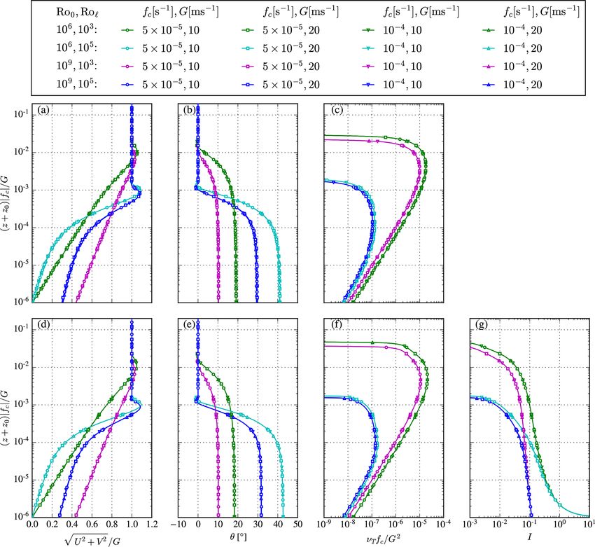
356                                     M. P. van der Laan et al.: Rossby number similarity of an atmospheric RANS model

mum turbulence length scale that is related to the ABL depth.
We show that the normalized profiles of wind speed, wind di-      DU                  d       dU
                                                                     = fc (V − VG ) +      νT      = 0,
rection and turbulence quantities are only dependent on two       Dt                  dz      dz
dimensionless parameters that represent the ratio of the in-      DV                     d

                                                                                                dV

ertial to the Coriolis force, based on two different length          = −fc (U − UG ) +       νT      = 0,                       (1)
                                                                  Dt                    dz      dz
scales: the roughness length and the maximum turbulence
length scale. These dimensionless parameters are Rossby           where U and V are the mean horizontal velocity compo-
numbers. The Rossby number based on the roughness length          nents, UG and VG are the corresponding mean geostrophic
is known as the surface Rossby number, as introduced by           velocities, fc = 2 sin(λ) is the Coriolis parameter with
Lettau (1959), while the Rossby number based on the max-          as Earth’s angular velocity and λ as the latitude, and z is the
imum turbulence length is a new dimensionless parameter.          height above ground. In addition, the Reynolds stresses u0 w 0
The obtained model-based Rossby number similarity is used         and v 0 w0 are modeled by the linear stress–strain relation-
to validate a range of simulations with historical measure-       ship of Boussinesq (1897): u0 w0 = −νT dU/dz and v 0 w0 =
ments of the geostrophic drag coefficient and cross-isobar an-    −νT dV /dz, where νT is the eddy viscosity. The boundary
gle. In addition, we show that both RANS models’ solutions        conditions for U and V are U = V = 0 at z = z0 and U = UG
are bounded by two analytic solutions of the idealized ABL.       and V = VG at z → ∞, where z0 is the roughness length.
   The limited-length-scale turbulence closures of Blackadar      Note that it is possible to write the two momentum equations
(1962) and Apsley and Castro (1997) can model the effect          as a single ordinary differential equation:
of stable and neutral stability but cannot model the unstable
atmosphere. We propose simple extensions to solve this is-

                                                                   d       dW
sue and validate the results of the extended k–ε model with             νT        = ifc W,                                    (2)
                                                                  dz        dz
measurements of wind speed and wind direction profiles.
The model extensions lead to a third Rossby number, where         where W ≡ (U − UG ) + i(V − VG ) is a complex variable and
the length scale is based on the Obukhov length. The lim-         i 2 = −1.
ited mixing-length model is not considered in the compari-            The eddy viscosity, νT , needs to be modeled in order to
son with measurements because we are mainly interested in         close the system of equations. The eddy viscosity can be
the limited-length-scale k–ε model. The k–ε model is more         written as νT = u∗ `, where u∗ and ` represent turbulence
applicable to wind energy applications because it can also        velocity and turbulence length scales. For a constant eddy
provide an estimate of the turbulence intensity, which is not     viscosity, the equations can be solved analytically, and the
available from the limited mixing-length model of Blackadar       solution is known as the Ekman spiral (Ekman, 1905), which
(1962). The limited mixing-length model is applied here to        includes the wind direction change with height due to Corio-
show that the same model-based Rossby number similarity           lis effects. The Ekman spiral can also be considered a laminar
as obtained for the k–ε model is recovered.                       solution, since one can neglect the turbulence in the momen-
   The article is structured as follows. The background and       tum equations and set the molecular viscosity to determine
theory of the idealized ABL are discussed in Sect. 2. Ex-         the rate of mixing. For an eddy viscosity that increases lin-
tensions to unstable surface layer stratification are presented   early with height, the equations can also be solved analyti-
in Sect. 3. Section 4 presents the methodology of the one-        cally, as introduced by Ellison (1956) and discussed by Kr-
dimensional RANS simulations. The model-based Rossby              ishna (1980) and Constantin and Johnson (2019). The two
similarity is illustrated in Sect. 5. The simulation results of   analytic solutions are provided in Appendix A. One can re-
the limited-length-scale k–ε model including the extension        late the analytic solution of Ellison (1956) to the (neutral)
to unstable conditions are compared with measurements in          ASL (z  zi ), while the Ekman spiral is more valid for alti-
Sect. 6.                                                          tudes around the ABL depth zi . Neither of the two analytic
                                                                  solutions result in a realistic representation of the entire (ide-
2   Background and theory – idealized models of                   alized) ABL. A combination of both a linear eddy viscosity
    the ABL                                                       for z  zi and a constant eddy viscosity for z ∼ zi should
                                                                  provide a more realistic solution. For example, the eddy vis-
We model the mean steady-state flow in an idealized ABL.          cosity could have the form νT = κu∗0 z exp(−z/ h), where
Here idealized refers to flow over homogeneous and flat ter-      νT increases linearly with height for z  h as expected in
rain under barotropic conditions such that the geostrophic        the surface layer; then it reaches a maximum value at z = h,
wind does not vary with height. This flow can be described by     and decreases to zero for z > h. Note that u∗0 is the friction
the incompressible RANS equations for momentum, where             velocity near the surface. Constantin and Johnson (2019) de-
the contribution from the molecular viscosity is neglected        rived a number of solutions for a variable eddy viscosity, al-
due to the high Reynolds number:                                  though an explicit solution for the entire idealized ABL with
                                                                  a realistic eddy viscosity (in the previously mentioned form)
                                                                  has not been found yet. Hence, numerical methods are still

Wind Energ. Sci., 5, 355–374, 2020                                                        www.wind-energ-sci.net/5/355/2020/
M. P. van der Laan et al.: Rossby number similarity of an atmospheric RANS model                                              357

necessary, and one of the simplest numerical models for the        the k–ε model of Apsley and Castro (1997) has an approx-
idealized ABL is given by Blackadar (1962) using Prandtl’s         imate dependence of zi ∝ (G/|fc |)1−a `amax with a ≈ 0.6,
mixing-length model:                                               which we will further discuss in Sect. 5. A summary of the
                                                                   discussed eddy viscosity closures is listed in Table 1. Fig-
νT = `2 S,                                                  (3)    ure 1 compares the analytic solutions of Ekman (1905) and
             p                                                     Ellison (1956) with the numerical solutions of the limited
where S = (dU/dz)2 + (dV /dz)2 = |dW/dz| is the magni-             mixing-length model of Blackadar (1962) and the limited-
tude of the strain-rate tensor, and ` is prescribed as a turbu-    length-scale k–ε of Apsley and Castro (1997) in terms of
lence length scale,                                                wind speed, wind direction, θ = arctan(V /U ), and eddy vis-
        κz                                                         cosity. The Ekman spiral is depicted with two constant eddy
`=            ,                                             (4)    viscosities, which only translates the solution vertically. In
     1 + `κz
          max
                                                                   addition, we have chosen fc = 10−4 s−1 , G = 10 m s−1 , and
where κz is the turbulence length scale in the neutral surface     z0 = 10−2 m. The numerical solutions are shown for a range
layer with κ as the von Kármán constant, and `max is a maxi-       of `max values. It is clear that the ABL depth decreases for
mum turbulence length scale. It is also possible to model the      lower values of `max , for both numerical models, and their so-
eddy viscosity with a two-equation turbulence closure, e.g.,       lutions behave similarly. A lower `max also results in a higher
the k–ε model:                                                     shear and wind veer and a lower eddy viscosity, which are
                                                                   characteristics of a stable ABL. Hence, the limited-length-
          k2                                                       scale turbulence closures can model the effects of stable strat-
νT = Cµ      ,                                              (5)
          ε                                                        ification by solely limiting the turbulence length scale, with-
with Cµ as a model parameter, k as the turbulent kinetic en-       out the need of a temperature equation or buoyancy source
ergy, and ε as the dissipation of k. Both k and ε are modeled      terms. When `max → 0 m (note that there is minimal limit
by a transport equation:                                           of `max in order to obtain numerically stable results), the so-
                                                                   lution approaches the Ekman spiral because the eddy viscos-
                                                                   ity in the ABL can be approximated by a constant eddy vis-

Dk      d νT dk
    =                + P − ε,                             (6)      cosity. Hence, the maximum change in wind direction simu-
Dt      dz σk dz
                                                                 lated by the k–ε model of Apsley and Castro (1997) is that of
Dε      d νT dε                         ε
    =                + Cε,1 P − Cε,2 ε ,                  (7)      the Ekman spiral: 45◦ . For large `max values, the numerical
Dt      dz σε dz                          k                        solution approximates the analytic solution of Ellison (1956)
where P is the turbulence production, and σk , σε , Cε,1 , and     but does not match it because their eddy viscosities are dif-
Cε,2 are model                                                     ferent for z ≥ zi .
              p constants that should follow the relation-
ship κ 2 = σε Cµ (Cε,2 − Cε,1 ). When using the standard
k–ε model calibrated for atmospheric flows (Richards and           3     Extension to unstable surface layer stratification
Hoxey, 1993), the turbulence length scale or eddy viscosity
will keep increasing until a boundary layer depth is formed        The two limited-length-scale turbulence closures discussed
and the analytic solution of Ellison (1956) is approximated.       in Sect. 2 can be used to model neutral and stable ABLs
Apsley and Castro (1997) proposed modifying the transport          without the need of a temperature equation and buoyancy
equation of ε, such that a maximum turbulence length scale         forces. However, it is not possible to model the unstable ABL
is enforced by replacing the constant Cε,1 with a variable pa-     because the turbulence length scale is only limited, not en-
          ∗ :
rameter Cε,1                                                       hanced, i.e., ` ≤ κz. In order to model unstable conditions,
                                                                   we need to extend the models such that the turbulence length
 ∗
                             `                                    scale is enhanced in the surface layer, ` > κz, which we
Cε,1 = Cε,1 + Cε,2 − Cε,1         ,                         (8)
                             `max                                  present in the following sections for each turbulence closure.

where the turbulence length scale is modeled as ` =
  3/4                                                              3.1    Limited mixing-length model
Cµ k 3/2 /ε. This limited-length-scale k–ε model behaves
very similarly to the mixing-length model of Blackadar             One can generically parameterize the turbulence length
(1962) (Eqs. 3 and 4). For `  `max , the surface layer so-        scale ` as a “parallel” combination of ASL and ABL scales,
lution is obtained, while for ` ∼ `max , the source terms in       1   1    1
the transport equation of ε cancel each other out (Cε,1 ∗ P ∼        =   +     .                                               (9)
                                                                   ` `ASL `ABL
Cε,1 ε), and the turbulence length scale is limited. For a
given z0 , G, and fc , the ABL depth can be controlled by `max .   Blackadar (1962) chose `ASL = κz and `ABL = `max to arrive
This means that `max is related to zi ; Apsley and Cas-            at Eq. (4). If we choose to set
tro (1997) noted that `max ∼ zi /3 applies to typical neutral               κz
ABLs. However, the simulated boundary layer depth using            `ASL =                                                (10)
                                                                            φm

www.wind-energ-sci.net/5/355/2020/                                                         Wind Energ. Sci., 5, 355–374, 2020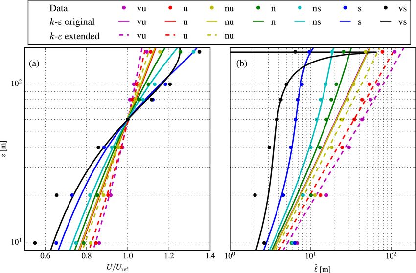
358                                        M. P. van der Laan et al.: Rossby number similarity of an atmospheric RANS model

Figure 1. Comparison of analytic and numerical solutions of existing idealized ABL models using fc = 10−4 s−1 , G = 10 m s−1 , and
z0 = 10−2 m for different model parameters. (a) Wind speed. (b) Wind direction. (c) Eddy viscosity.

Table 1. Eddy viscosity closures for the idealized ABL.

                                    Eddy viscosity closure                              Solution      Reference
          Constant                           –                –                         Analytic      Ekman (1905)
          Linear                             νT = u∗0 `       ` = κz                    Analytic      Ellison (1956)
          Limited mixing-length model        νT = `2 S        ` = κz/ (1 + κz/`max ),   Numerical     Blackadar (1962)
                                                                   3/4
          Limited-length-scale k–ε model     νT = Cµ k 2 /ε   ` = Cµ k 3/2 /ε           Numerical     Apsley and Castro (1997)

following the turbulence length scale that is a result of              Thus we can simply use the original length-scale model of
Monin–Obukhov Similarity Theory (MOST, Monin and                       Blackadar (1962) for stable and neutral conditions; the stable
Obukhov, 1954) – where                                                 φm function simply informs the selection of `max,eff , follow-
                                                                       ing Eq. (13).
φm = (1 − γ1 z/L)−1/4                                         (11)
is the dimensionless velocity gradient for unstable condi-             3.2   Limited-length-scale k –ε model
tions, with γ1 ≈ 16 as shown by Dyer (1974), and L is the
Obukhov length – then it is possible to extend the limited             Sumner and Masson (2012) argued that, in stable condi-
mixing-length model of Blackadar (1962) to unstable surface            tions, the limited-length-scale k–ε model of Apsley and Cas-
layer stratification, as                                               tro (1997) overpredicts ` in the surface layer compared to
                                                                       MOST, where `max = Lκ/β and β ≈ 5. They proposed a
                   κz                                                  more complicated expression for Cε,1 ∗ in the transport equa-
`=                 −1/4
                                  .                    (12)
     (1 − γ1 z/L)       + κz/`max                                      tion of ε compared to the original model of Apsley and Cas-
                                                                       tro (1997). Sogachev et al. (2012) alternatively prescribed a
Approaching neutral conditions, L−1 → 0, the original
                                                                       coefficient in the buoyant term of the ε equation, depending
length-scale model of Blackadar (1962) is obtained. Note
                                                                       on `/`max and being similar to the production-related term
that in stable conditions, φm = 1+βz/L, so the resulting tur-
                                                                       that gives results consistent (at least asymptotically) with
bulence length can also be rewritten in the form of Eqs. (4)
                                                                       MOST. We find that the correction of Sumner and Masson
and (9), using an effective maximum turbulence length scale
                                                                       (2012) provides a better match of the turbulence length scale
of
                                                                       within the surface layer compared to MOST with respect to
`−1            −1         −1
 ABL,stable = `max,eff ≡ `max + β/(κL).                       (13)     the original k–ε model of Apsley and Castro (1997). How-

Wind Energ. Sci., 5, 355–374, 2020                                                             www.wind-energ-sci.net/5/355/2020/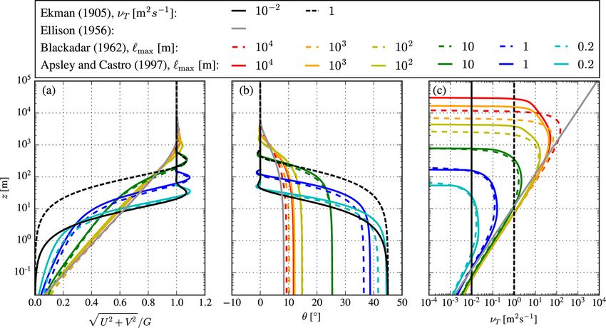
M. P. van der Laan et al.: Rossby number similarity of an atmospheric RANS model                                                       359

ever, we also find that a larger overshoot of the turbulence       4.1   Ambient turbulence in the limited-length-scale k –ε
length scale around the ABL depth is found when Coriolis is              turbulence model
included. Alternatively, one could improve the surface layer
solution of the original model of Apsley and Castro (1997) by      The limited-length-scale k–ε model typically simulates an
simply reducing `max by roughly 20 %. Therefore, we choose         eddy viscosity that decays to zero for z → ∞, which can lead
to use the model of Apsley and Castro (1997) as our starting       to numerical instability. While, for example, Koblitz et al.
point.                                                             (2015) chose to set upper limits for k and ε to prevent numeri-
   In order to account for the increase in turbulence length       cal instabilities, we prefer a more physical method, including
scale in the surface layer under unstable conditions, we add       ambient source terms Sk,amb and Sε,amb in the k and ε trans-
a buoyancy source term B in the k–ε transport equations:           port equations, respectively. Following Spalart and Rumsey
                                                                   (2007), we set

Dk      d νT dk
     =                + P − ε + B,                       (14)                                        2
                                                                                                    εamb
 Dt     dz σk dz                                                   Sk,amb = εamb , Sε,amb = Cε,2         .                             (19)
Dε

        d νT dε

                                                ε                                                  kamb
                          ∗                ∗
     =                + Cε,1 P − Cε,2 ε + Cε,3 B .       (15)
 Dt     dz σε dz                                 k                 When all sources of turbulence are zero (P = B = 0) and the
                                                                   diffusion terms are zero (dk/dz = dε/dz = 0), then k = kamb
Here B is modeled as
                                                                   and ε = εamb . To be consistent with the equations solved, we
         "                #
            dU 2

                       dV 2 z               z                      define the ambient turbulence quantities in terms of the driv-
B = −νT            +            , = −νT S 2                (16)    ing parameters, G and `max :
            dz         dz     L             L
                                                                                              3 2
following MOST, using the similarity functions of Dyer             `amb = Camb `max , kamb = Iamb G2 ,
                                                                                              2
(1974) as discussed in van der Laan et al. (2017). We use the                   3
                            ∗ ≡ 1 + α (C                                                          3
                                                                                              r
flow-dependent parameter Cε,3           B ε,1 − Cε,2 ) of So-
                                                                                2                       3
                                                                           3/4 kamb      3/4 3 3 Iamb G
gachev et al. (2012), which for unstable conditions includes       εamb = Cµ         = Cµ                  .                           (20)
                                                                               `amb          2 2 Camb `max
the prescription
          "                 #                                     Here Iamb is the total turbulence intensity1 above the (sim-
                  Cε,2 − 1       `                                 ulated) ABL, and Camb is the ratio of the turbulence length
αB = 1 − 1 +                       ,                    (17)
                 Cε,2 − Cε,1 `max                                  scale above the ABL (`amb ) to maximum turbulence length
                                                                   scale (`max ). We choose small values for Iamb = 10−6 and
amenable to the free-convection limit: ε/B → 1 for P/B →           Camb = 10−6 , such that the ambient turbulence does not af-
0. Further, αB → 1 as ` → 0, matching neutral conditions           fect the solution for U and V , while the numerical stability
since z/L also vanishes then. The prescription (Eq. 17) re-        is maintained. It should be noted that the overshoot in `/`max
sults in                                                           that can occur near the ABL depth is still affected by the am-
                                          `                       bient values. Sogachev et al. (2012) and Koblitz et al. (2015)
 ∗
Cε,3 = 1 + Cε,1 − Cε,2 + 2Cε,2 − Cε,1 − 1      ,           (18)    chose to use a limiter on ε to avoid an overshoot in `, but we
                                          `max
                                                                   choose not to use it. In general, we prefer to avoid limiters
which also means that C∗ε,3 → Cε,2 approaching the effec-          because they can break the Rossby number similarity that is
tive ABL top (` → `max ), so sources and sinks of ε balance        presented in Sect. 5.
in Eq. (15), i.e., P −ε +B, all have the same coefficient Cε,2 .
                                                                   4.2   Numerical setup
4   Methodology of numerical simulations
                                                                   The flow is driven by a constant pressure gradient using a
The one-dimensional numerical simulations are performed            prescribed constant geostrophic wind speed. The initial wind
with EllipSys1D (van der Laan and Sørensen, 2017a), which          speed is set to the geostrophic wind speed at all heights. Dur-
is a simplified one-dimensional version of EllipSys3D, ini-        ing the solving procedure, the ABL depth grows from the
tially developed by Sørensen (1994) and Michelsen (1992).          ground until convergence is achieved, which occurs when the
EllipSys1D is a finite volume solver for incompressible flow,      growth rate of the ABL depth is negligible because a balance
with collocated storage of flow variables. It is assumed that      between the prescribed pressure gradient, the Coriolis forces,
the vertical velocity is zero and the pressure gradients are       and the turbulence stresses is obtained. The flow that we are
constant, which is valid in an idealized ABL, as discussed         solving is relatively stiff, and we choose to include the tran-
in Sect. 2. As a consequence, it is not necessary to solve the     sient terms using a second-order three-level implicit method
pressure correction equation that is normally used to ensure          1 From the two-equation k–ε model (which is isotropic), the total
mass conservation.                                                                                             √        p
                                                                   turbulence intensity is calculated by I =       2/3k/ U 2 + V 2 .

www.wind-energ-sci.net/5/355/2020/                                                          Wind Energ. Sci., 5, 355–374, 2020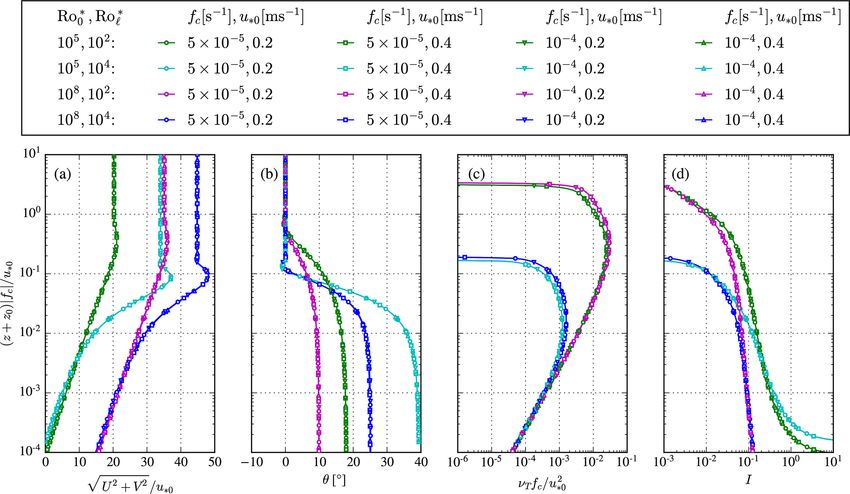
360                                         M. P. van der Laan et al.: Rossby number similarity of an atmospheric RANS model

with a large time step that is set as 1/|fc | s. All spatial gra-       5   Rossby number similarity in numerical and
dients are discretized by a second-order central-difference                 analytical solutions
scheme. Convergence is typically achieved after 105 itera-
tions, which takes about 10 s on a single 2.7 GHz CPU. The              The numerical solution of the original limited-length-scale
domain height is set to 105 m to ensure that the ABL depth              turbulence closures of Blackadar (1962) and Apsley and Cas-
is significantly smaller than the domain height for all flow            tro (1997) depend on four parameters: fc (s−1 ), G (m s−1 ),
cases considered. The numerical grid represents a line, where           `max (m), and z0 (m). Applying the Buckingham π theorem,
the first cell height is set to 10−2 m. The cells are stretched         it is clear that there should exist two dimensionless numbers
for increasing heights using an expansion ratio of about 1.2.           that define the entire solution, since the four dimensional pa-
The grid consists of 384 cells, which is based on a grid re-            rameters only have two dimensions (meters and seconds).
finement study presented in Sect. 4.3. A rough-wall bound-              This can be shown by writing a nondimensional momentum
ary condition is set at the ground, as discussed by Sørensen            equation in complex form (Eq. 2) using the nondimensional
et al. (2007). For the length-scale-limited k–ε model, this             variables W 0 ≡ W/U, νT0 ≡ νT /(UL) and z0 ≡ z/L, where
means that we set ε at the first cell, use a Neumann con-               U and L are characteristic velocity and length scales, respec-
dition for k, and the shear stress at the wall is defined by            tively:
the neutral surface layer. The first cell is placed on top of
                                                                                      dW 0

the roughness length, which allows us to choose the first cell                d
                                                                        Ro 0 νT0             = iW 0 .                             (21)
height independent of the roughness length. This means that                  dz        dz0
we add the roughness length to all relations that include z,
i.e., z + z0 . For the limited mixing-length model, we simply           Here, Ro is the Rossby number, Ro = U/(|fc |L), which de-
set the eddy viscosity from the neutral surface layer at the            scribes the ratio of the inertial (advective) tendency to the
first cell. Neumann conditions are set for all flow variables at        Coriolis force. If we apply the original mixing-length model
the top boundary.                                                       of Blackadar (1962) for νT0 using Eqs. (3) and (4), then
   The turbulence model constants of the k–ε model are set as           Eq. (21) can be written as
(Cµ , σk , σε , Cε,1 , Cε,2 , κ) = (0.03, 1.0, 1.3, 1.21, 1.92, 0.4).                             2             !
                                                                                         κz0          dW 0 dW 0

The chosen Cµ value is based on neutral ASL measurements,                    d
                                                                        Ro 0                                        = iW 0 ,     (22)
as discussed by Richards and Hoxey (1993), and Cε,1 is used                 dz     1 + κz0 L/`max      dz0 dz0
to maintain the neutral ASL solution of the k–ε model.
                                                                        where −L/`max , is a second dimensionless number. If we
4.3   Grid refinement study                                             choose U = G and L = z0 , we may define two Rossby-
                                                                        like numbers, with characteristic length scales based on z0
A grid refinement study of the numerical setup is performed             and `max , respectively:
for the limited-length-scale k–ε model of Apsley and Cas-
tro (1997), using 48, 96, 192, 384, and 768 cells. We choose                       G                 G
                                                                        Ro0 ≡            , Ro` ≡           .                        (23)
fc = 10−4 s−1 , z0 = 10−4 m, and G = 10 m s−1 for `max =                         |fc |z0         |fc |`max
100 and `max = 1 m. The results in terms of the wind speed
of each grid are depicted in Fig. 2 for both values of `max . For       Here, we have obtained Ro` by rewriting the second dimen-
`max = 100 m, the largest difference with respect to the finest         sionless number L/`max as the ratio of the two Rossby num-
grid is 0.5 %, 0.2 %, 0.09 %, and 0.03 % for 48, 96, 192, and           bers: L/`max = [U/(|fc |`max )]/[U/(|fc |L)]. Ro0 is known
384 cells, respectively, located at the first cell near the wall        as the surface Rossby number, first introduced by Lettau
boundary. When using `max = 1 m, a small ABL depth of                   (1959); it also resembles a ratio of (inertial) boundary layer
100 m is simulated with a sharp low-level jet. In the enlarged          depth to z0 . Analogously, Ro` is like the ratio of two bound-
plot of Fig. 2b, one can see how the grid size affects the low-         ary layer depths, fc /u∗0 and zi (e.g., Arya and Wyngaard,
level jet, where the largest difference with respect to the finest      1975); here `max is a proxy for zi , acting as a “lid” for the
grid is 1 %, 0.2 %, 0.04 %, and 0.01 %, for 48, 96, 192, and            ABL. Considering Eq. (23), we have reduced the number
384 cells, respectively. We find similar results for the limited        of dependent parameters from four to two: f (fc , G, `max ,
mixing-length model of Blackadar (1962). In addition, the               z0 ) → f (Ro0 , Ro` ). For a fixed surface roughness z0 , the ra-
turbulence model extensions to unstable surface layer strati-           tio of the two Rossby numbers is then the only dependent
fication typically show smaller differences between the grids           parameter:
due to the enhanced mixing and the use of a high `max value                      Ro0
that represents a convective ABL. Hence, our choice of using            `max =       z0 ;                                           (24)
                                                                                 Ro`
384 cells is conservative.
                                                                        i.e., the ratio of simulated ABL depth to z0 is the lone param-
                                                                        eter. Blackadar (1962) found a characteristic maximum ABL
                                                                        turbulence length scale of 0.00027 G/|fc | for the Leipzig

Wind Energ. Sci., 5, 355–374, 2020                                                              www.wind-energ-sci.net/5/355/2020/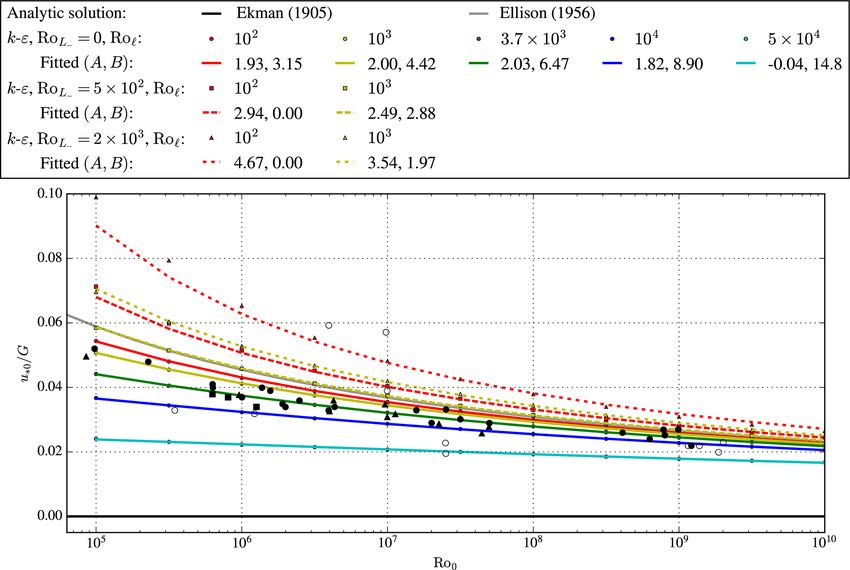
M. P. van der Laan et al.: Rossby number similarity of an atmospheric RANS model 361
Figure 2. Grid refinement study of the one-dimensional RANS simulation using the limited-length-scale k–ε model, for 48, 96, 192, 384, and
768 cells. (a) `max = 100 m. (b) `max = 1 m.
wind profile (Lettau, 1950), which equating with `max cor- here the subscript (L− ) denotes that Eq. (25) is defined for
responds to Ro` ' 3700. unstable conditions, i.e., L ≤ 0. For the convective boundary
Figure 3 depicts the Rossby number similarity of layer, u∗0 /(−|fc |L) is generally replaced by the dimension-
our one-dimensional RANS simulations using the origi- less inversion height −zi /L, because the convective ABL
nal limited-length-scale turbulence closures of Blackadar depth does not have a significant dependence on u∗0 /fc
(1962), Fig. 3a–c, and Apsley and Castro (1997), Fig. 3d– (Arya, 1975). However, we note that RoL− functions as a
g. Four combinations of Ro0 (106 and 109 ) and Ro` (103 “bottom-up” parameter in the non-neutral RANS equation
and 105 ) are used, each simulated with four combinations set, with the Obukhov length L in Eq. (16) specified as a
of G (10 and 20 m s−1 ) and fc (5 × 10⁻⁵ and 10−4 s−1 ). surface layer quantity; in effect RoL− dictates the relative
The roughness length and maximum turbulence length scale increase in mixing length (i.e., in the dimensionless coordi-
follow from Eq. (23) and cover a wide range of z0 from nate z|fc |/G). Our length-scale-limited turbulence closures
10−4 to 0.4 m and `max of 100–400 m. Figure 3 shows that extended to unstable surface layer stratification, as presented
normalized wind speed, wind direction, and turbulence quan- in Sect. 3, are dependent on RoL− . This becomes clear when
tities for both turbulence closures are only dependent on Ro0 we substitute the mixing-length model extended to unstable
and Ro` . Both turbulence closures produce similar results in surface layer stratification from Eq. (12) into the nondimen-
terms of wind speed, wind direction, and eddy viscosity. The sional momentum equation from Eq. (21):
limited-length-scale k–ε model of Apsley and Castro (1997) 2 !
κz0 dW 0 dW 0
also predicts a total turbulence intensity I (Fig. 3g) and a d
Ro = iW 0 , (26)
turbulence length scale ` (not shown in Fig. 3), which are dz0 (1 − γ1 z0 L/L)−1/4 + κz0 L/`max dz0 dz0
only dependent on the two Rossby numbers. In addition, the
total turbulence intensity close to the surface only depends where L/L is a third nondimensional number, which can also
on Ro0 , while further away, it is mainly influenced by Ro` be written as the ratio of two Rossby numbers: RoL− /Ro0 .
with a weaker dependence on Ro0 . For RoL− = 0, the extended models return to the original
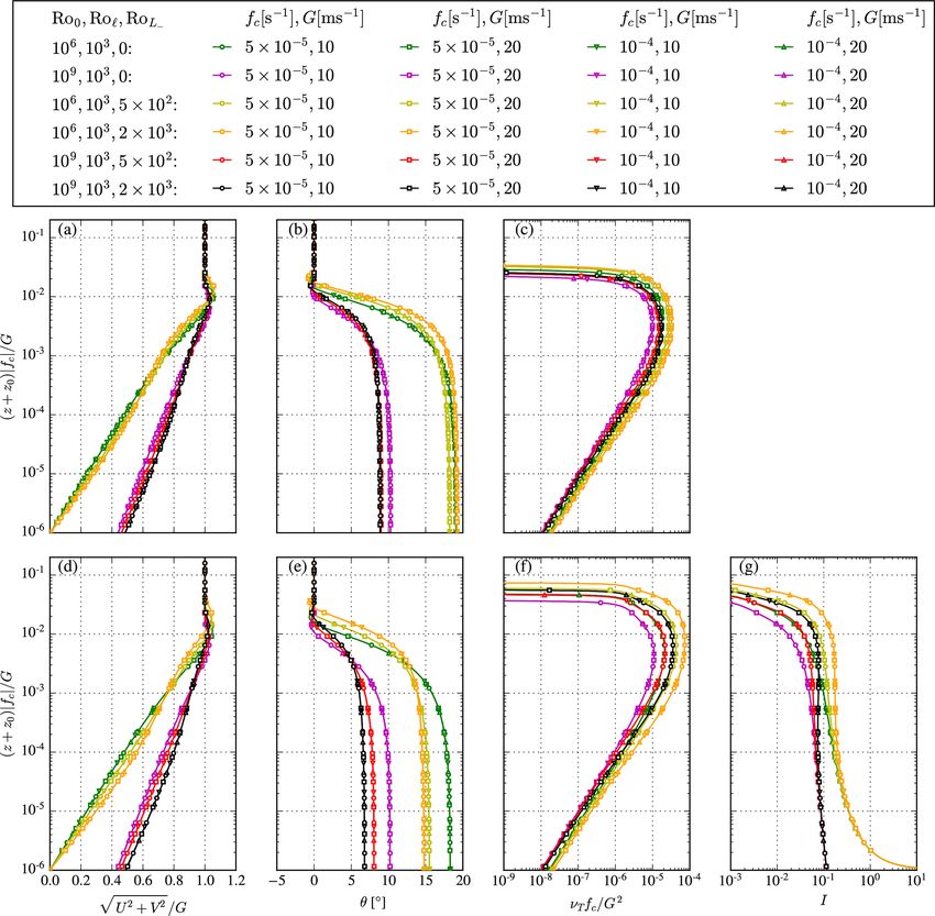
Considering the non-neutral ABL with Coriolis effects models. Figure 4 depicts the Rossby number similarity of the
but ignoring the strength of capping inversion (entrain- extended turbulence closures using six combinations of the
ment), in the micrometeorological literature the Kazanskii three Rossby numbers, which are each simulated with four
and Monin (1961) parameter u∗0 /(|fc |L) is typically invoked combinations of G and fc . We use two values of Ro0 (106
(e.g., Arya, 1975; Zilitinkevich, 1989). This can also be con- and 109 ) and three values of RoL− (0, 5×10² , and 2×10³ ) for
sidered as a third Rossby number, which in our context of Ro` = 103 . For these Rossby number combinations, RoL− =
using G instead of u∗0 is 5×10² and RoL− = 2×10³ correspond to near-unstable con-
ditions (−1/L = 0.00125–0.005 m−1 ) and unstable to very
−G unstable conditions (−1/L = 0.005–0.02 m−1 ), respectively.
RoL− ≡ ; (25) Figure 4 shows that both extended turbulence closures only
|fc |L
www.wind-energ-sci.net/5/355/2020/ Wind Energ. Sci., 5, 355–374, 2020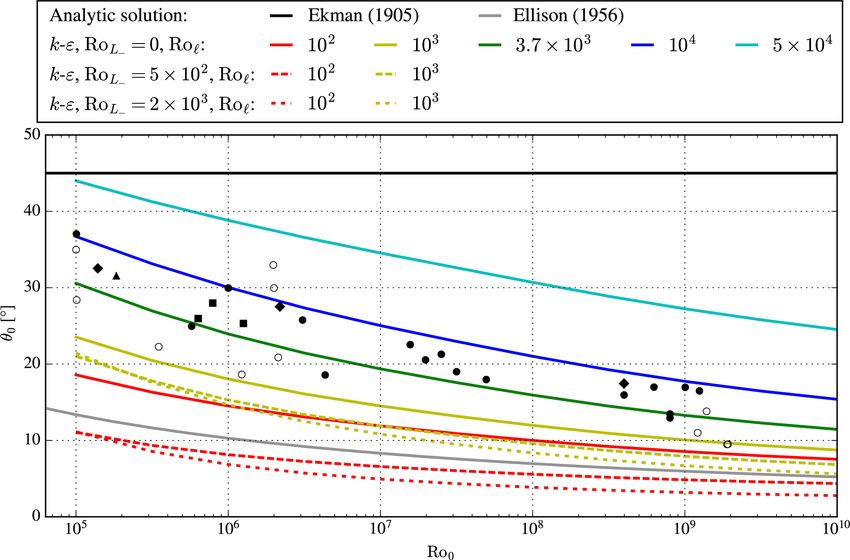
362                                       M. P. van der Laan et al.: Rossby number similarity of an atmospheric RANS model

Figure 3. Rossby number similarity of the original turbulence closures. (a–c) Limited mixing-length model. (d–g) Limited-length-scale k–ε
model.

depend on Ro0 and RoL− for a given Ro` . Although not                  it does not always decrease with increasing unstable condi-
shown in Fig. 4, changing Ro` would not break the Rossby               tions for the extended mixing-length model (Fig. 4b).
number similarity. Note that it does not make sense to include            One could choose to use the friction velocity at the sur-
combinations of nonzero values of RoL− that correspond to              face, u∗0 , as a velocity scale in the Rossby numbers instead
unstable conditions and large values of Ro` that correspond            of the geostrophic wind speed. However, the friction velocity
to stable conditions.                                                  depends on height z and is a result of the model, not an input.
   The extended limited-length-scale mixing-length model               In other words, the height at which the friction velocity needs
(Fig. 4a–c) is less sensitive to RoL− compared to the ex-              to be extracted to obtain a collapse is also dependent on the
tended limited-length-scale k–ε model (Fig. 4d–g) because              ABL profiles, since the height scales with friction velocity.
of the buoyancy production in the transport equations of k             Hence it is more sensible to use geostrophic wind speed as a
and ε, which is not present in the extended mixing-length              velocity scale in the model-based Rossby number similarity
model. Both models predict a deeper ABL (larger zi ) that is           – consistent also with classic Ekman theory (which relates
more mixed for stronger unstable surface layer stratification          the wind speed in terms of G). Nevertheless, it is possible
(increasing RoL− ). The wind veer is also reduced in stronger          to obtain a Rossby similarity using u∗0 as the velocity scale,
unstable conditions for the extended k–ε model (Fig. 4e), but          which is presented in Appendix B.

Wind Energ. Sci., 5, 355–374, 2020                                                             www.wind-energ-sci.net/5/355/2020/

M. P. van der Laan et al.: Rossby number similarity of an atmospheric RANS model                                                   363

Figure 4. Rossby number similarity of the turbulence closures extended to unstable surface layer conditions. (a–c) Limited mixing-length
model. (d–g) Limited-length-scale k–ε model.

   The Rossby number similarity can be employed to gen-                  The ABL depth zi predicted by the original limited-length-
erate a library of ABL profiles for a range of Ro0 , Ro` ,            scale turbulence closures is mainly dependent on the max-
and RoL− . The library contains all possible model solutions          imum turbulence length scale `max . The normalized ABL
for the range of chosen Rossby numbers, and it can be used to         depth ((zi + z0 )|fc |/G) is mainly dependent on Ro` , which
determine inflow profiles for three-dimensional RANS sim-             is depicted in Fig. 5, where results of the limited-length-
ulations, without the need for running one-dimensional pre-           scale k–ε model extended to unstable surface layer strati-
cursor simulations.                                                   fication are shown for 3 × 6 × 3 combinations of the three
   The obtained Rossby number similarity can only be                  Rossby numbers Ro0 , Ro` , and RoL− . We have chosen
achieved for a grid-independent numerical setup, as we have           G = 10 m s−1 and fc = 10−4 s−1 , but the results are inde-
shown in Sect. 4.3. In addition, the ambient source terms             pendent of G and fc due to the Rossby number similarity.
should also be scaled by the relevant input parameters (G and         The normalized ABL depth is defined as the height at which
`max ), as discussed in Sect. 4.1.                                    the wind direction (relative to the geostrophic wind direction)
                                                                      becomes zero for the second time, i.e., above the mean jet and

www.wind-energ-sci.net/5/355/2020/                                                             Wind Energ. Sci., 5, 355–374, 2020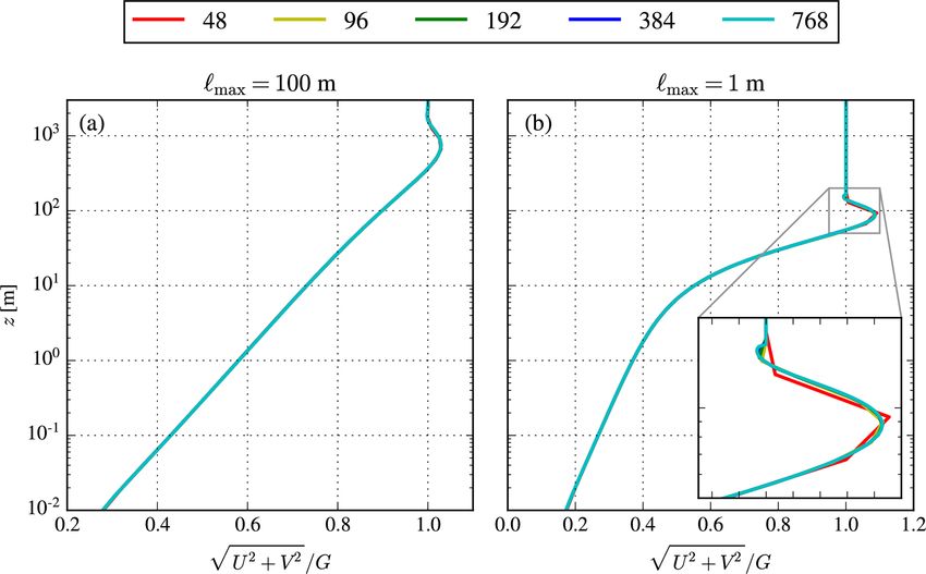
364                                       M. P. van der Laan et al.: Rossby number similarity of an atmospheric RANS model

                                                                      the comparison with measurements, since we are mainly in-
                                                                      terested in the k–ε model.

                                                                      6.1   Geostrophic drag coefficient
                                                                      The geostrophic drag law (GDL) is a widely used relation in
                                                                      boundary layer meteorology and wind resource assessment
                                                                      (after Troen and Petersen, 1989), which connects the surface
                                                                      layer properties as z0 and u∗0 with the driving forces on top
                                                                      of the ABL proportional to |fc |G:
                                                                                s
                                                                                                 2
                                                                            u∗0          u∗0
                                                                      G=           ln            − A + B 2,                    (27)
                                                                             κ         |fc |z0

                                                                      where A and B are empirical constants. The GDL can be de-
                                                                      rived from Eq. (1), where the Reynolds stresses do not need
                                                                      to be modeled explicitly (as in, for example, Zilitinkevich,
                                                                      1989) and can be expressed as an implicit relation for the
Figure 5. Normalized boundary layer depth zi predicted by limited-    geostrophic drag coefficient u∗0 /G and Ro0 :
length-scale k–ε model extended to unstable surface layer stratifi-
cation, as a function of the three Rossby numbers.                    u∗0                   κ
                                                                          = q                              .                    (28)
                                                                       G                             2
                                                                              ln (Ro0 ) + ln uG∗0 − A + B 2


associated turning as in Ekman theory. For the Ekman solu-
tion (Sect. A1),                                                         Figure 6 is a reproduction from Hess and Garratt (2002),
            √ this definition results in an ABL depth equal           where the geostrophic drag coefficient is depicted as a func-
to zi = 2π 2νT /|fc |. The normalized ABL depth in the
RANS model increases for stronger unstable surface layer              tion of surface Rossby number Ro0 . The black markers
conditions (larger RoL− ), i.e., for larger values of the sur-        are measurements summarized by Hess and Garratt (2002),
face heat flux. For neutral and stable conditions (RoL− =             where the dots are near-neutral and near-barotropic condi-
0) and moderate to shallow ABL depths, i.e., 3 × 10³ ≤                tions, the triangles and squares reflect less idealized atmo-
Ro` ≤ 3 × 10⁴ – corresponding to zi
M. P. van der Laan et al.: Rossby number similarity of an atmospheric RANS model 365
Figure 6. Reproduced from Hess and Garratt (2002). Geostrophic drag coefficient simulated by the limited-length-scale k–ε model extended
to unstable surface layer stratification, taken at a normalized height of (z+z0 )|fc |/G = 5×10⁻⁵ (i.e., in the surface layer), for different Ro0 ,
Ro` , and RoL− . Black markers represent measurements from Hess and Garratt (2002). Ro` = 3.7 × 10³ represents `max from Blackadar
(1962). Analytic results of Ekman (1905) and Ellison (1956) are summarized in Appendix A.
In addition, the extension to unstable surface layer conditions that the GDL from Eq. (27) limits how large B can be; gener-
can also explain the trend of the more uncertain measure- ally u∗0 /G < κ/B, so values of B greater than those shown
ments (black dots). Since Ro` and RoL− influence the ABL are not physical. The model results in Fig. 6 do not violate
depth, as previously shown in Fig. 5, the model suggests that this limit.
the measurements were conducted for a range of ABL depths
that could reflect a range of atmospheric stabilities, although
6.2 Cross-isobar angle
the geostrophic wind shear can play a role here as shown by
Floors et al. (2015). Figure 7 is a reproduction of Hess and Garratt (2002), where
The fitted A and B parameters in Fig. 6 are dependent the angle between surface wind direction and the geostrophic
on Ro` and RoL− , which both influence the ABL depth. This wind direction is plotted as a function of the surface Rossby
is not a surprising result, since many authors have shown number. This angle is known as the cross-isobar angle, θ0 .
that A and B are dependent on atmospheric stability (see, for The black markers, analytic solutions, and model results fol-
example, Arya, 1975; Zilitinkevich, 1989; Landberg, 1994). low the same definition as used in Fig. 6, where additional
For moderate roughness lengths over land, the measured val- black diamond markers are added that correspond to clima-
ues tabulated by Hess and Garratt (2002) generally fall be- tological measurements, as discussed by Hess and Garratt
tween the blue and yellow lines for neutral conditions, which (2002). For RoL− = 0, the model results of the cross-isobar
are consistent with the typically used values in wind energy, angle are bounded by the analytic solutions, as also found for
i.e., A = 1.8 and B = 4.5 (e.g., Troen and Petersen, 1989). the geostrophic drag coefficient in Fig. 6. All measurements
Assuming `max is a measure of the ABL depth, then in the summarized by Hess and Garratt (2002) can be simulated
actual atmosphere over land we have Ro0 /Ro` ∼ 103 –105 , by the limited-length-scale k–ε model by varying the ABL
while over sea the ratio is roughly 106 –107 . Thus one can see depth using Ro` . Most of the measurements are well pre-
that the typical wind energy values of A and B are a compro- dicted for RoL− = 0 and Ro` = 103 –104 , which is the range
mise for applicability over both land and sea. The real-world used by Blackadar (1962) (Ro` = 3.7 × 10³ ). For RoL− 6= 0,
limits mean that the result for Ro` = 102 (red line) can ex- smaller values of the cross-isobar angle can be simulated
tend only from Ro0 ∼ 105 –107 , while the over-sea regime compared with the analytic solution of Ellison (1956) due to
(large Ro0 ) tends to involve a smaller range of Ro` . We note the enhanced rate of mixing. The model cannot predict larger
www.wind-energ-sci.net/5/355/2020/ Wind Energ. Sci., 5, 355–374, 2020366 M. P. van der Laan et al.: Rossby number similarity of an atmospheric RANS model
Figure 7. Reproduced from Hess and Garratt (2002). Cross-isobar angle simulated by the limited-length-scale k–ε model extended to
unstable surface layer stratification, taken at a normalized height of (z + z0 )|fc |/G = 5 × 10⁻⁵ for different Ro0 , Ro` , and RoL− . Black
markers represent measurements from Hess and Garratt (2002). Ro` = 3.7 represents `max from Blackadar (1962). Analytic results of Ekman
(1905) and Ellison (1956) are summarized in Appendix A.
values of the cross-isobar angle compared to the analytic so- taking the wind speed at 40, 60, and 80 m. The fitted pa-
lution of Ekman (1905) (45◦ ). rameters are obtained by running the numerical simulations
with a gradients-based optimizer, and the results are listed
6.3 Atmospheric surface layer profiles in Table 2. The maximum `max is set to 103 m, which cor-
responds to an ABL depth on the order of 5 km, as depicted
Peña et al. (2014) used measurements of the wind speed com- in Fig. 5. The unstable cases are also simulated with the ex-
ponents from 10 to 160 m, from The National Test Station for tended limited-length-scale k–ε model using the measured L
Wind Turbines at Høvsøre, a coastal site in Denmark, charac- and refitted G and `max , which are listed in Table 2 as values
terized as flat grassland. The Coriolis parameter for the test in parentheses.
location is 1.21 × 10⁻⁴ s−1 . The measurements were taken Figure 8 depicts the wind speed and turbulence length
from sonic anemometers over 1 year, and a wind direction scale of the measurements and numerical simulations us-
sector was selected to avoid the influence of the coastline ing the original and extended limited-length-scale k–ε mod-
and wind turbine wakes. Peña et al. (2014) also calculated els. The turbulence length scale from the numerical simu-
a “mixing” (turbulence) length scale `ˆ using a local friction lation is calculated by Eq. (29), instead of the usual defi-
velocity u∗ and the wind speed gradient: 3/4
nition ` = Cµ k 3/2 /ε. The original limited-length-scale k–
u∗ ε model of Apsley and Castro (1997) can capture the wind
`ˆ = . (29)
dU/dz speed and turbulence length scale for the stable and neutral
cases. Note that for the very stable case, the shear is underes-
Seven cases were defined based on the atmospheric stability,
timated and the model predicts an ABL depth of about 100 m,
and these are listed in Table 2 in terms of the Obukhov length, ˆ since dU/dz is zero around the
which results in a spike in `,
roughness length, and friction velocity. In order to apply the
ABL depth. As expected, the original limited-length-scale
limited-length scale k–ε, we need to set the geostrophic wind
k–ε model cannot predict a lower shear and a larger turbu-
speed and the maximum turbulence length scale, which are
lence length scale compared to neutral atmospheric condi-
both unknown. We choose to use G and `max as free param-
tions (where dU/dz = u∗ /` and ` = κz), and the optimizer
eters, which we fit to a reference wind speed and a turbu-
used to fit G and `max sets `max to our chosen maximum
lence length scale, at a reference height of 60 m. The wind
value of 103 m. Note that therefore the lines corresponding
speed gradient is obtained from a central-difference scheme
Wind Energ. Sci., 5, 355–374, 2020 www.wind-energ-sci.net/5/355/2020/M. P. van der Laan et al.: Rossby number similarity of an atmospheric RANS model 367
Table 2. ASL validation cases. Fitted G, fitted `max , and modeled u∗0 in parentheses represent values for the extended model.
Data Model
1/L z0 u∗0 Fitted G Fitted `max u∗0
Case (m−1 ) (m) (m s−1 ) (m s−1 ) (m) (m s−1 )
Very unstable (vu) −1.35 × 10⁻² 1.3 × 10⁻² 0.35 8.00 (7.50) 103 (5.39 × 10² ) 0.30 (0.34)
Unstable (u) −7.04 × 10⁻³ 1.2 × 10⁻² 0.41 10.1 (9.56) 103 (5.54 × 10² ) 0.37 (0.40)
Near unstable (nu) −3.18 × 10⁻³ 1.2 × 10⁻² 0.40 10.3 (10.0) 103 (2.00 × 10² ) 0.37 (0.39)
Neutral (n) 1.87 × 10⁻⁴ 1.3 × 10⁻² 0.39 11.0 4.01 × 101 0.37
Near stable (ns) 3.14 × 10⁻³ 1.2 × 10⁻² 0.36 11.3 1.72 × 101 0.35
Stable (s) 9.61 × 10⁻³ 0.8 × 10⁻² 0.26 9.96 6.49 × 100 0.27
Very stable (vs) 3.57 × 10⁻² 0.2 × 10⁻² 0.16 8.62 3.35 × 100 0.20
Figure 8. ASL measurements of Peña et al. (2010) compared to simulation results of the original limited-length-scale k–ε model of Apsley
and Castro (1997). (a) Wind speed. (b) Turbulence length scale from Eq. (29). Unstable cases are also simulated with our extension to
unstable surface layer stratification with L from Table 2.
to unstable conditions of the original k–ε model largely over- It should be noted that the validation presented in
lap in Fig. 8. Higher values of `max would not improve the Fig. 8 could be considered as a best-possible simulation-
results. The limited-length-scale k–ε model extended to un- to-measurement comparison because we have allowed our-
stable surface layer stratification is able to predict turbulence selves to tune both G and `max . When G is provided by the
length scales larger than ` = κz and shows improved results measurements, it is more difficult to obtain a good match, as
for both the shear and the turbulence length scale. shown in Sect. 6.4.
Table 2 also shows the measured and simulated friction
velocity at a height of 10 m. The simulated friction velocity is
2 2 6.4 Atmospheric-boundary-layer profiles
calculated as u∗ = (u0 w0 +v 0 w0 )1/4 . For the unstable cases,
it is clear that the extended model predicts friction velocities Peña et al. (2014) performed lidar measurements of the hori-
that are closer to the measurements compared to the original zontal wind speed components from 10 to 1200 m at the same
limited-length-scale k-ε model due to the enhanced mixing. test site as discussed in Sect. 6.3. Peña et al. (2014) selected
10 cases that differ in geostrophic forcing and atmospheric
www.wind-energ-sci.net/5/355/2020/ Wind Energ. Sci., 5, 355–374, 2020368 M. P. van der Laan et al.: Rossby number similarity of an atmospheric RANS model
Table 3. ABL validation cases based on Peña et al. (2014).
Case Description 1/L G z0 u∗0 Ro0 RoL−
(m−1 ) (m s−1 ) (m) (m s−1 ) (–) (–)
4 Stable, strongly forced 4.5 × 10⁻³ 20.5 1.6 × 10⁻² 0.45 1.0 × 10⁷ –
5 Neutral −5 × 10⁻⁴ 19.5 1.6 × 10⁻² 0.70 1.0 × 10⁷ –
9 Very unstable, weak forcing −4.0 × 10⁻² 5.02 1.6 × 10⁻² 0.26 2.8 × 10⁶ 1.7 × 10³
stability. The cases were selected to challenge the valida- Esau (2005), the “mid-ABL” scale of Gryning et al. (2007)
tion of numerical models. Since our numerical setup can (generalized by Kelly and Troen (2016) for matching G), and
only handle a constant geostrophic wind speed, we select the the “top-down” scale of Kelly et al. (2019).
barotropic cases from Peña et al. (2014): cases 4, 5, and 9 and Figure 9 depicts the measured wind speed and wind direc-
the corresponding values of the Obukhov length, geostrophic tion, for each validation case. Since cases 4 and 5 have the
wind, roughness length, friction velocity, Ro0 , and RoL− are same G (within 5 %) and thus same surface Rossby number
listed in Table 3. For convenience, we keep the case names Ro0 ' 107 , we can plot them together because the normal-
as introduced by Peña et al. (2014). Cases 4 and 5 represent ized model results are the same for both cases. The error
a stable and a neutral ABL with high forcing, respectively, bars represent the standard error of the mean. The original
where Ro0 = 107 . Case 9 is characterized by a low forcing limited-length-scale k–ε model of Apsley and Castro (1997)
and very unstable stratification, where Ro0 = 2.8 × 10⁶ . is employed with a range of Ro` . The unstable ABL case
In Case 6 from Peña et al. (2014) it is observed that the (Case 9) is also simulated with the model extension to un-
lidar measurements do not approach the geostrophic wind stable surface layer stratification using RoL− from Table 3
speed at large heights above the surface. This is because the and the two smallest values of Ro` . Case 4 has a strong
geostrophic wind speed in Peña et al. (2014) is derived from wind shear and a wind veer that leads to a cross-isobar an-
outputs of the Weather Research and Forecasting (WRF) gle of 50◦ . The limited-length-scale k–ε model can predict
model over a large area, potentially leading to bias. There- a maximum cross-isobar angle of 45◦ for extremely shal-
fore, we use a slightly different approach to estimate the low ABL depths, as shown in Sect. 6.2. Hence, the measured
geostrophic wind; because the wind speed above the ABL ABL from Case 4 is not a possible numerical solution. The
is nearly always in geostrophic balance we can just assume measured ABL from Case 5 can be predicted by the origi-
the wind speed measured by the wind lidar above the bound- nal limited-length-scale k–ε model, while this is not the case
ary layer depth to be equal to the geostrophic wind speed, for the wind speed close to the ground of Case 9 due to the
thereby avoiding possible prediction errors in wind speed strong unstable stratification. When the limited-length-scale
from the WRF model. Instead, only the ABL depth is es- k–ε model including the extension for unstable surface layer
timated from the WRF model outputs. The ABL depth is conditions is employed, the prediction of the wind speed near
available as a diagnostic variable predicted by the Yonsei the ground is improved, although it is difficult to correctly
University ABL scheme (Hong et al., 2006) in the WRF predict both wind speed and wind direction. It should be
model. To be sure that the lidar wind speed is close to the noted that the extended (unstable) model only improves the
geostrophic wind speed, we always estimate it from the level wind speed in the surface layer (at 10 m), noting the dotted
that is higher than the modeled ABL depth during all 30 min and solid lines crossing in Fig. 9c.
means, which constitute the three cases. From the measurements during Case 9 it was observed that
Since G is known, we can use Rossby similarity for model the WRF-modeled ABL depth grew from 300 m to nearly
validation. While one could try to find an `max to get the best 1200 m, which indicates that the conditions were largely
comparison with the measurements, we find that it is difficult transient; such nonstationary conditions are difficult for a
to define a good metric. For example, we could attempt to RANS model. More unstable cases are necessary to further
find an `max that results in an equivalent ABL depth equal to validate the extended model, including measurements of tur-
that of the measurement cases; however, the ABL depth was bulence quantities such as the (total) turbulence intensity.
not directly measured and only estimated from a model. In- It is possible to use validation cases based on turbulence-
stead of finding a single `max value, we choose to simulate a resolving methods, such as large-eddy simulations, in future
range of `max values. We note that part of this difficulty is due work.
to the limited extent of the model. There is no “top-down” in-
formation; i.e., we lack entrainment effects and the impact of
the strength of the capping inversion. An extra length scale
could be introduced to account for such effects; examples are
the nonlocal static stability scale found in Zilitinkevich and
Wind Energ. Sci., 5, 355–374, 2020 www.wind-energ-sci.net/5/355/2020/M. P. van der Laan et al.: Rossby number similarity of an atmospheric RANS model 369
Figure 9. ABL measurements from Peña et al. (2014) compared to simulation results of the original limited-length-scale k–ε model of
Apsley and Castro (1997), for a range of Ro` . (a, c) Wind speed. (b, d) Wind direction. Unstable Case 9 (c, d) is also simulated with our
extension to unstable surface layer stratification (dashed lines), with RoL− (i.e., 1/L) from Table 3.
7 Conclusions surements of relevant associated meteorological quantities,
such as the geostrophic drag coefficient and cross-isobar an-
gle. The measured variation in these measurements can be
The idealized ABL was simulated with a one-dimensional
explained by dependence upon the new Rossby number (i.e.,
RANS solver, using two different turbulence closures: a
ABL depth). In addition, we have shown how two classic an-
limited mixing-length model and a limited-length-scale k–
alytic solutions of the idealized ABL (Ekman, 1905; Ellison,
ε model. While these models require four input parameters,
1956) act as bounds on the results obtainable by the limited-
we have shown that the simulated ABL profiles collapse to
length-scale k–ε model.
a dependence upon two Rossby numbers, which are defined
The limited-length-scale turbulence closures can repre-
by the roughness length and the maximum turbulence length
sent the effects of stable and neutral stratification but cannot
scale, respectively. The Rossby number based on the maxi-
model unstable conditions. We have proposed simple exten-
mum turbulence length scale is a new dimensionless number
sions to overcome this issue, without adding a temperature
and is related to the ABL depth. The model-based Rossby
equation (van der Laan et al., 2017). The extended models
number similarity obtained herein is valid for both turbu-
require an additional input, the Obukhov length, which can
lence models. We have employed Rossby number similarity
be used to define a third Rossby number. We have shown
to compare the range of model solutions with historical mea-
www.wind-energ-sci.net/5/355/2020/ Wind Energ. Sci., 5, 355–374, 2020370 M. P. van der Laan et al.: Rossby number similarity of an atmospheric RANS model that the extension of the k–ε model compares well with mea- The application of the one-dimensional RANS simulations surements of seven ASL profiles, representing a range of at- to generate inflow profiles for three-dimensional RANS sim- mospheric stabilities, including three unstable cases. The k– ulations is not performed here and it should be investigated ε model further offers turbulence intensity, whose profile is in future work. Ongoing and future work also includes the also found to collapse according to the developed similarity incorporation of the effect of the capping-inversion strength theories. A model validation of the ABL for a stable, a neu- to accommodate entrainment at the ABL top (softening the tral, and an unstable case is performed, with less success for ABL lid, one might say); this can be considered as an intro- the non-neutral cases. In the very stable case, the measured duction of an additional length scale. In addition, the effects wind veer of 50◦ was larger than the maximum wind veer of length-scale limitation and neglecting the buoyancy force of 45◦ that the k–ε model can simulate. In addition, the very in the momentum equation need to be quantified for three- unstable case was characterized by nonstationary conditions, dimensional RANS simulations of complex terrain and wind which are difficult to capture with a RANS model. More val- farms. idation cases based on the convective ABL are necessary to quantify the performance of the turbulence model extension to unstable conditions beyond the surface layer. Wind Energ. Sci., 5, 355–374, 2020 www.wind-energ-sci.net/5/355/2020/
You can also read