Variability of the thermohaline structure and transport of Atlantic water in the Arctic Ocean based on NABOS Nansen and Amundsen Basins Observing ...
←
→
Page content transcription
If your browser does not render page correctly, please read the page content below
Ocean Sci., 16, 405–421, 2020
https://doi.org/10.5194/os-16-405-2020
© Author(s) 2020. This work is distributed under
the Creative Commons Attribution 4.0 License.

Variability of the thermohaline structure and transport of Atlantic
water in the Arctic Ocean based on NABOS (Nansen and
Amundsen Basins Observing System) hydrography data
Nataliya Zhurbas and Natalia Kuzmina
Shirshov Institute of Oceanology, Russian Academy of Sciences, 36 Nakhimovsky Prospekt, 117997 Moscow, Russia

Correspondence: Nataliya Zhurbas (nvzhurbas@gmail.com)

Received: 16 May 2019 – Discussion started: 3 June 2019
Revised: 26 January 2020 – Accepted: 3 February 2020 – Published: 2 April 2020

Abstract. Conductivity–temperature–depth (CTD) transects         the St. Anna Trough, and 1.1 Sv in the longitude range 94–
across continental slope of the Eurasian Basin and the           107◦ E.
St. Anna Trough performed during NABOS (Nansen and
Amundsen Basins Observing System) project in 2002–2015
and a transect from the 1996 Polarstern expedition are used      1   Introduction
to describe the temperature and salinity characteristics and
volume flow rates (volume transports) of the current carrying    Atlantic water (AW) enters the Eurasian Basin in two
the Atlantic water (AW) in the Arctic Ocean. The variability     branches (see, e.g., Aagaard, 1981; Rudels et al., 1994, 1999,
of the AW on its pathway along the slope of the Eurasian         2006, 2015; Schauer et al., 1997, 2002a, b; Berzczynska-
Basin is investigated. A dynamic Fram Strait branch of the       Möller et al., 2012; Rudels, 2015; Dmitrenko et al., 2015;
Atlantic water (FSBW) is identified in all transects, includ-    Pnyushkov et al., 2015, 2018b): one branch originates from
ing two transects in the Makarov Basin (along 159◦ E), while     the Greenland and Norwegian seas and flows to the basin
the cold waters on the eastern transects along 126, 142, and     through Fram Strait (the Fram Strait branch of the Atlantic
159◦ E, which can be associated with the influence of the        water, hereinafter the FSBW), and the other reaches the deep
Barents Sea branch of the Atlantic water (BSBW), were ob-        part of the Arctic Ocean near St. Anna Trough after pass-
served in the depth range below 800 m and had a negligi-         ing through the Barents Sea (the Barents Sea branch of the
ble effect on the spatial structure of isopycnic surfaces. The   Atlantic water, hereinafter the BSBW). After entering the
geostrophic volume transport of AW decreases farther away        Eurasian Basin the FSBW moves eastward with a subsur-
from the areas of the AW inflow to the Eurasian Basin, de-       face boundary current and has a core of higher tempera-
creasing by 1 order of magnitude in the Makarov Basin at         ture and salinity than the BSBW. In the longitude range of
159◦ E, implying that the major part of the AW entering the      80–90◦ E, it encounters and partially mixes with the BSBW,
Arctic Ocean circulates cyclonically within the Nansen and       which is strongly cooled due to mixing with shallow waters
Amundsen basins. There is an absolute maximum of θmax            of the Arctic shelf seas and atmospheric impact (Schauer et
(AW core temperature) in 2006–2008 time series and a max-        al., 1997, 2002a, b). Further, the water masses resulting from
imum in 2013, but only at 103◦ E. Salinity S(θmax ) (AW core     the interaction of the two branches spread cyclonically in the
salinity) time series display a trend of an increase in AW       Eurasian Basin.
salinity over time, which can be referred to as an AW salin-        Within the NABOS (Nansen and Amundsen Basins Ob-
ization in the early 2000s. The maxima of θmax and S(θmax )      serving System) project (Polyakov et al., 2007) a unique vol-
in 2006 and 2013 are accompanied by the volume transport         ume of conductivity–temperature–depth (CTD) data was col-
maxima. The time average geostrophic volume transports of        lected: more than 30 sections were made in various regions
AW are 0.5 Sv in the longitude range 31–92◦ E, 0.8 Sv in         of the Arctic Basin in summer and fall 2002–2015. A num-
                                                                 ber of sections in different years were made in the same re-

Published by Copernicus Publications on behalf of the European Geosciences Union.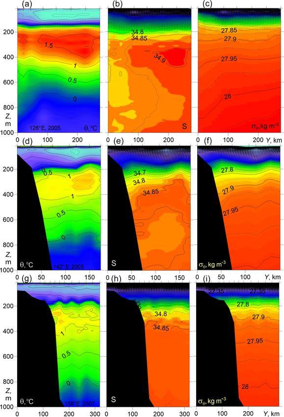
406 N. Zhurbas and N. Kuzmina: Variability of the thermohaline structure and transport of Atlantic water
gions of the basin, which allows studying the interannual ers with warm and fresh water (which cannot be attributed to
variability of the water masses thermohaline structure and AW) were excluded. For the observations of BSBW in the St.
the geostrophic volume flow rate in these areas. Anna Trough the geostrophic transport was calculated by in-
The main goal of this work is to investigate the spatial tegration over a depth range with temperature below 0 ◦ C and
and temporal variability of the AW geostrophic volume flow salinity above 34.5. If both AW branches were present on the
rate during its propagation along the continental slope of the transect, the integration was performed over the entire depth
Eurasian Basin. We further discuss the thermohaline struc- range but excluding the cold near-surface layer (θ < 0 ◦ C)
ture and transformation of the FSBW and BSBW. The esti- and the warm (θ > 0 ◦ C) and relatively fresh (S < 34.5) near-
mates of the AW transport are sensitive to the temperature surface layer. The zero-velocity depth in this case was chosen
and salinity ranges used for the identification of this water after inspection of the observed pattern of density contours,
(Pnyushkov et al., 2018b), and mixing of FSBW, BSBW and i.e., suggesting either the near-surface flow pattern or the
surrounding waters may change the AW geostrophic volume near-bottom flow pattern (see Sect. 3). The details and limi-
transport along the slope. tation of the geostrophic velocity calculations are discussed
in Zhurbas (2019).
2 Material and methods
3 Results
We used data from the CTD transects across the slope of the
Eurasian Basin in the longitude range of 31–159◦ E measured 3.1 Variability of the thermohaline pattern on the AW
in the years 2002–2015 within the framework of the NABOS pathway along the slope of the Eurasian Basin
project (in total 39 transects). The data are freely available
at the site http://nabos.iarc.uaf.edu (last access: 24 January 3.1.1 CTD transect analysis
2019, IARC, 2019). In addition, a CTD transect across the
entire Eurasian Basin and over the Lomonosov Ridge start- The transformation of thermohaline signatures (i.e., patterns
ing at 92◦ E at the slope from R/V Polarstern in 1996 (here- of salinity S, potential temperature θ, and potential den-
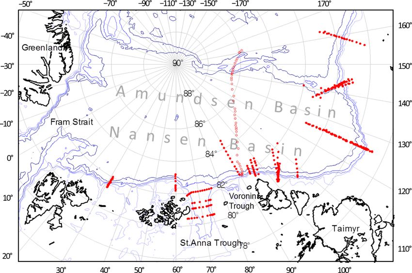
after PS96) was also included. The locations of the CTD tran- sity anomaly σθ vs. cross-slope distance and depth) of the
sects are shown in Fig. 1. Most of the transects are aligned AW flow on its pathway along the slope of the Eurasian
cross-slope and grouped at longitudes of 31, 60, 90, 92, 94, Basin are presented in Fig. 2. The σθ contours in transects
96, 98, 103, 126, 142, and 159◦ E. Four of the 40 transects at 31◦ E diverge towards the continental slope margin (to
crossed zonally the St. Anna Trough (at the latitude of 81, the south), shallowing above the warm and saline core of
81.33, 81.42, and 82◦ N) through which the BSBW enters the AW and sloping down beneath it associated with a east-
the Eurasian Basin. Most of the CTD casts covered the up- ward subsurface flow. Such a distribution of isopycnic sur-
per layer from the sea surface to either 1000 m depth or to faces was observed on all NABOS transects taken across an
the bottom (if the total depth was shallower). Approximately available continental slope at 31◦ E. According to Fig. 2 the
every third or fourth cast was down to the sea bottom even if warm and saline core of the Fram Strait branch of the AW
the sea depth exceeded 1000 m. with the maximum temperature θmax of 4.88 ◦ C at the depth
To estimate the volume transport of the Atlantic water, Zθmax = 102 m and the maximum salinity Smax of 35.11 at the
we applied standard dynamical method. The no-motion level depth ZSmax = 176 m is found on the slope at about 1000 m
(the depth of zero velocity) was determined from the follow- isobath.
ing consideration. If the baroclinic current occupies the upper Figure 3 presents temperature, salinity, and potential den-
layer or/and some intermediate layer, the no-motion level can sity for two zonal transects across the St. Anna Trough at
be chosen in a calm deep layer (where the horizontal density latitudes of 81 and 82◦ N. A stable pool of cold (θ < 0 ◦ C)
gradient is relatively small). By contrast, in case of a near- and dense (σθ > 28 kg m−3 ) water in the bottom layer is seen
bottom gravity flow, the no-motion level can be reasonably adjacent to the eastern slope of the trough. The transfer of
chosen well above the near-bottom flow. For the level of no- the densest water pool to the eastern slope corresponds to
motion, we adopted either 1000 m depth or the sea bottom a geostrophically balanced near-bottom gravity flow to the
depth, if the latter was smaller than 1000 m for the FSBW, north. This near-bottom gravity current also carries waters
and approximately 50 m, where density contours were more of Atlantic origin, which are strongly cooled due to mixing
or less flat, for the observations of BSBW in the St. Anna with shelf waters in the Barents and Kara seas. Above the
Trough (see also below). near-bottom gravity flow of the BSBW one can observe a
Since the FSBW brings saline and warm water to the two-core structure of warm FSBW with temperature up to
Eurasian Basin, the geostrophic transport was found by in- 2.5 ◦ C that enters the St. Anna Trough from the northwest
tegration over the depth range with positive temperature, at the western side of the trough and leaves it for the north-
θ > 0 ◦ C, and relatively high salinity, S > 34.5 (the salinity is east at the eastern side of the trough. At 82◦ N, the BSBW
given in the practical salinity scale); that is, near-surface lay- overflows a ridge-like elevation east of the St. Anna Trough
Ocean Sci., 16, 405–421, 2020 www.ocean-sci.net/16/405/2020/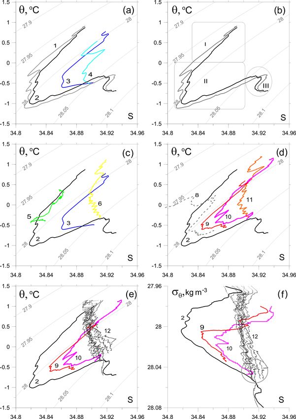
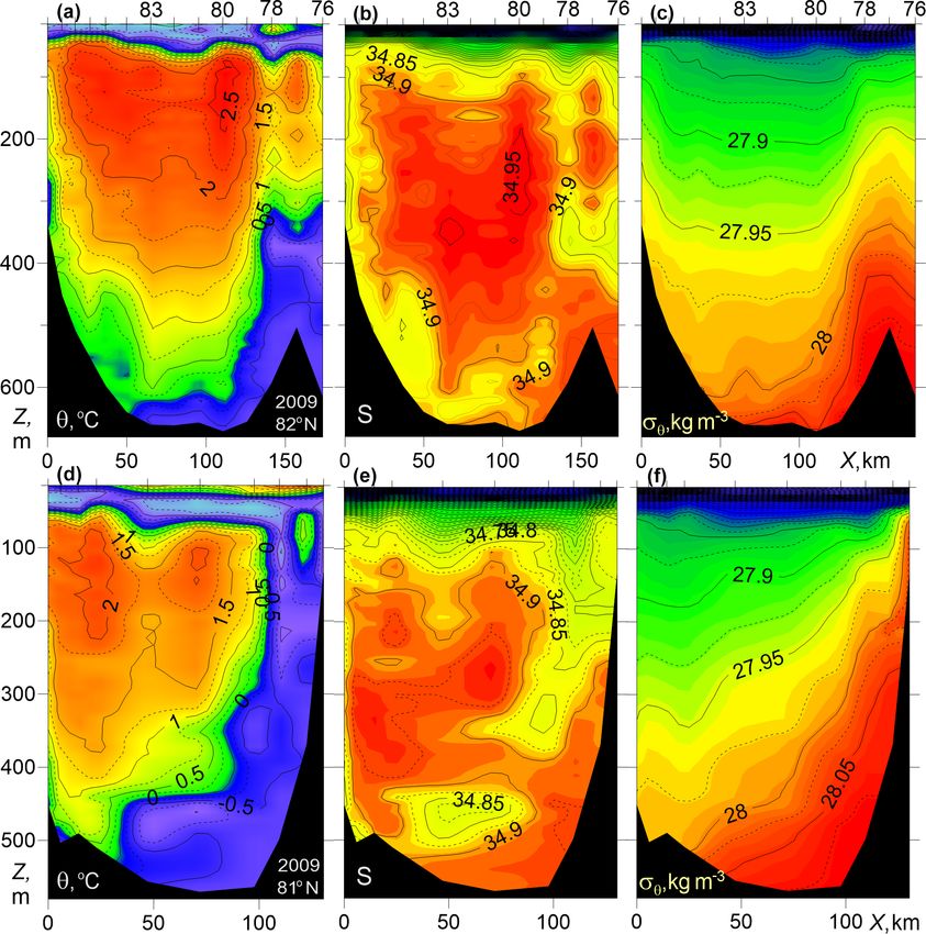
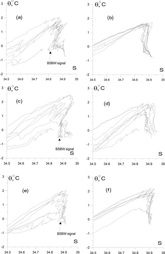
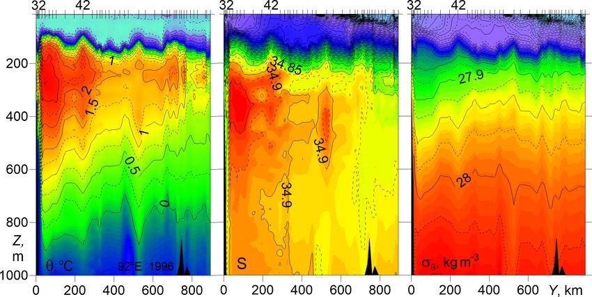
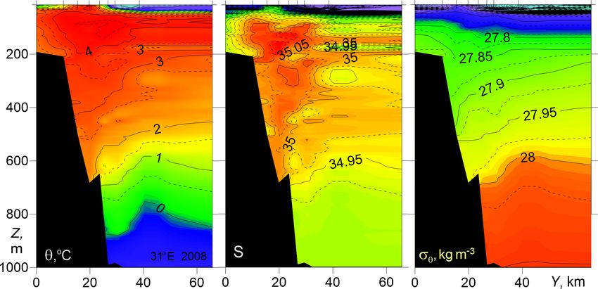
N. Zhurbas and N. Kuzmina: Variability of the thermohaline structure and transport of Atlantic water                                407

Figure 1. Bathymetric map of the Eurasian Basin with 300, 500, 1000, and 2000 m contours shown. The red filled and blank circles are the
locations of CTD stations on the NABOS and PS96 transects, respectively.

Figure 2. Temperature θ , salinity S, and potential density anomaly σθ vs. cross-slope distance and depth for the NABOS08 transect across
the Eurasian Basin slope at 31◦ E. Locations of the CTD stations are shown in the transects at the top. Here and hereinafter the NABOS
expedition references are abbreviated: for example NABOS08 corresponds NABOS-2008.

(Fig. 3a–c). Studies of the currents and hydrography in the            be identified by −2 ◦ C < θ < 0 ◦ C, 34.75 < S < 34.95, and
St. Anna Trough can be found in Schauer et al. (2002a, b),             27.8 kg m−3 < σθ < 28.0 kg m−3 . Other approaches to define
Rudels et al. (2015), and Dmitrenko et al. (2015).                     BSBW are given in Schauer et al. (1997, 2002a, b) and
   In order to understand the effect of the FSBW and the               Dmitrenko et al. (2015). According to Schauer et al. (1997,
BSBW transformation on geostrophic volume flow rate, it                2002a, b) the BSBW includes all waters that enter the Nansen
is necessary to identify water masses of different origin. For         Basin from the St. Anna and Voronin troughs. The temper-
that purpose the following criterion is often used (Walsh et           ature of these waters, however, can reach ∼ 1 ◦ C. The jus-
al., 2007; Pfirman et al., 1994): the water masses of the              tification for this approach was based on θ –S analysis of
FSBW are characterized by θ > 0 ◦ C, and the BSBW can                  the waters of the northeastern part of the Barents Sea and

www.ocean-sci.net/16/405/2020/                                                                        Ocean Sci., 16, 405–421, 2020
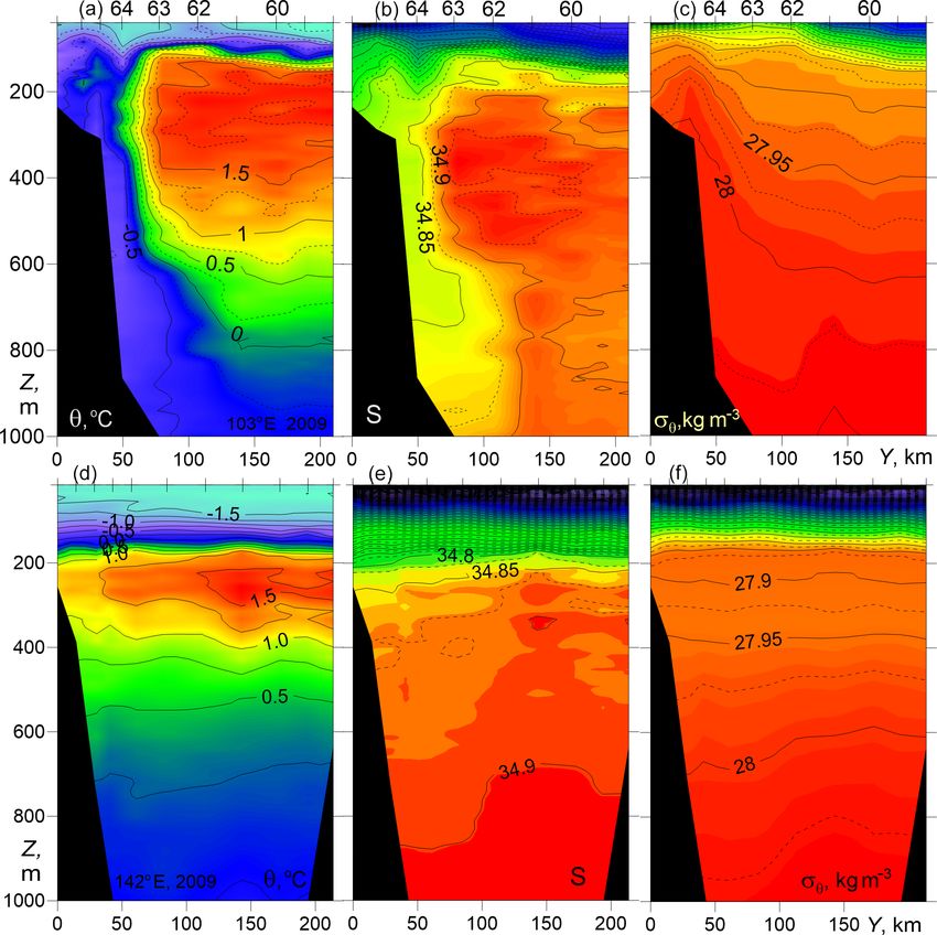
408               N. Zhurbas and N. Kuzmina: Variability of the thermohaline structure and transport of Atlantic water

Figure 3. Temperature θ , salinity S, and potential density anomaly σθ vs. distance and depth for zonal transects across the St. Anna Trough
at latitudes of 81◦ N (d–f, NABOS09) and 82◦ N (a–c, NABOS09). The x axis is directed to the east. Numbers at the top indicate numbers
of the CTD stations.

the St. Anna and Voronin troughs. According to Dmitrenko                despite the masking effect of vertical undulations of σθ con-
et al. (2015), the BSBW consists of two water masses, and               tours caused by internal waves and mesoscale eddies (one
the temperature of the warmer water mass can only slightly              of subsurface, intra-pycnocline eddies is probably identified
exceed 0 ◦ C (for more details, see Sect. 3.1.2). Here we will          at the distance of Y = 510 km), isopycnals tend to shoal or
rely on the definitions of the FSBW and BSBW proposed by                deepen above or below the FSBW core towards the continen-
Dmitrenko et al. (2015).                                                tal slope margin (to the south) which, in terms of geostrophic
   In Fig. 4 the CTD transect at 92◦ E carried out in the 1996          balance, implies the eastward flow of FSBW. The FSBW
Polarstern expedition just east of the entrance point of the            core in the 92◦ E transect is found at 40 km distance from
BSBW to the Eurasian Basin from the St. Anna Trough and                 the slope, with the maximum temperature θmax = 2.79 ◦ C at
Voronin Trough is presented. It can be assumed that a part              Zθmax = 271 m and salinity Smax = 34.97 at ZSmax = 329 m.
of the BSBW extends deep into the basin, mixing with the                Therefore, the FSBW on its pathway along the slope of the
FSBW, while another part of the BSBW flows eastward along               Eurasian Basin from 31 to 92◦ E has cooled, desalinated,
the slope according to the general cyclonic circulation ob-             sunk, and become denser by about 2 ◦ C, 0.1, 150 m, and
served in the Eurasian Basin. On the presented transect the             0.1 kg m−3 , respectively. Another distinct feature in the PS96
BSBW is observed in the depth range below 600 m as a nar-               transect is a layer with increased temperature between 180
row, about 10 km wide strip of cold water near the slope (see           and 300 m depth at Y = 600–750 km in the vicinity of the
also Sect. 3.1.2) adjacent to a 300 km wide zone occupied by            Lomonosov Ridge, which can be attributed to the geostroph-
the warm FSBW. The potential density distribution of FSBW               ically balanced FSBW return flow cyclonically circulating
in this transect is similar to transects at 31◦ E. That is to say,

Ocean Sci., 16, 405–421, 2020                                                                         www.ocean-sci.net/16/405/2020/
N. Zhurbas and N. Kuzmina: Variability of the thermohaline structure and transport of Atlantic water                         409

around the Eurasian Basin (Rudels et al., 1994; Swift et          occupied by the FSBW. As the FSBW moved along the con-
al., 1997).                                                       tinental slope of the Eurasian Basin, its core temperature de-
   According to Schauer et al. (2002b), who studied the PS96      creased but could be identified at all transects, including the
section, the horizontal and vertical scales of the BSBW were      two transects in the Makarov Basin (159◦ E). The cold wa-
taken at 30 km and 800 m, respectively. This differs from our     ters in the transects along 126, 142, and 159◦ E, which can
interpretation based on the definition of BSBW with temper-       be associated with the BSBW, had a minimum temperature
ature less than 0 ◦ C.                                            above −0.5 ◦ C, were located below 800 m, and had relatively
   Further east, in the longitude range of 94–107◦ E (NA-         flat isopycnic surfaces.
BOS09), the denser part of BSBW under the FSBW is char-
acterized by an eastward geostrophic current with isopycnals      3.1.2   θ –S analysis
sloping towards the north in a 150 km wide zone adjacent
to the slope (see Fig. 5a–c). Less-saline water at the slope      The difficulty in identifying the BSBW in the eastern part of
is the less dense BSBW that has entered the Nansen Basin          the Nansen Basin is related to the overlapping ranges of tem-
when the slope narrows north of Severnaya Zemlya (Schauer         perature and salinity inherent to the BSBW and the UPDW:
et al., 1997).                                                    −0.5 ◦ C < θ < 0 ◦ C, and the salinity is close to 34.9 (Rudels
   The vertical location of the FSBW layer is similar to 92◦ E    et al., 1994; Walsh et al., 2007). It is also important to note
in the section PS96, but the maximum temperature has fur-         that the BSBW in the St. Anna Trough mixes with the FSBW.
ther decreased: in the transect in Fig. 5a–c, θmax = 1.98 ◦ C     Therefore, it is not only the cold Atlantic waters, which are
at Zθmax = 245 m and Smax = 34.95 at ZSmax = 365 m. Fig-          transported by the bottom gravity current, but also mixed
ure 5d–f present the transect at 142◦ E (NABOS09) which           warmer waters that can enter the Nansen Basin through the
is located on the Lomonosov Ridge, between the Amund-             trough (see Fig. 3). A detailed θ –S analysis of different CTD
sen and Makarov basins. The comparison of the two tran-           sections can provide useful information on the transport and
sects obtained in the same year shows that the vertical scale     transformation of FSBW and BSBW. A distinct θ –S signa-
of the warm FSBW (θ > 1.5 ◦ C) has significantly decreased.       ture indicates that the water mass has entered the area of ob-
Nevertheless, the FSBWs are also observed at this longitude       servation. The absence of a signature in the θ –S space indi-
and affect the slopes of isopycnic surfaces in a layer up to      cates either that the water mass did not enter the area of ob-
300 m. The cold waters with θ < 0 ◦ C, which can be associ-       servation or that it was transformed after mixing with other
ated with the BSBW, are observed only at two stations in the      waters.
depth range close to 1000 m and are absent at depths above           The differences in the behavior of the θ –S values are ob-
950 m. The isopycnic surfaces in Fig. 5d–f are relatively flat,   served in the upper and deep layers of the Eurasian Basin
indicating weak geostrophic flow (see Sect. 3.2). The “abso-      and the St. Anna Trough (Fig. 7). On the other hand, one
lutely stable” thermohaline stratification below the tempera-     cannot miss a similarity in the shape of the θ –S curves in
ture maximum with temperature decreasing and salinity in-         the salinity range of 34.5–35.0. The similarity is obviously
creasing with depth (Fig. 5d–f) is common in the Upper Polar      caused by the presence of FSBW. Figure 7 demonstrates the
Deep Water (UPDW) layer (Rudels et al., 1999).                    transformation of the FSBW and BSBW moving along the
   In Fig. 6 three transects are presented, at 126 and 142◦ E     continental slope of the Eurasian Basin. More detailed infor-
(NABOS05) and in the Makarov Basin at 159◦ E (NA-                 mation on the BSBW transformation can be extracted from
BOS07). On the transect along 126◦ E large slopes of isopy-       θ –S diagrams presented in Fig. 8.
cnic surfaces are observed, which corresponds to a fairly            The θ–S curves marked as 1 and 2 in Fig. 8a correspond
strong geostrophic flow (see Sect. 3.2), confined to the depth    to stations 76 and 78, respectively, which were located at the
range of 200–400 m, that is, to the area occupied by the          eastern slope of the St. Anna Trough just in the near-bottom
FSBW. At the 142◦ E transect on the Lomonosov Ridge and           gravity current carrying the BSBW, while the curves marked
at the 159◦ E transect in the Makarov Basin, the FSBW can         as 3 and 4 correspond to stations 83 and 80 located near the
be still identified as a warm layer between 200 and 400 m,        midpoint (thalweg) of the trough in the western periphery
where the maximum temperature is reduced to 1.49 and              of the gravity current (the location of the stations is shown
1.42 ◦ C, respectively (Fig. 6). The 142◦ E transect implies      in Fig. 3). To visualize the BSBW transformation better, the
some eastward geostrophic transport, whereas at the 159◦ E        points of θ –S curves in the temperature and salinity ranges of
transect and in the area of cold waters (below 800 m) in the      θ > 1.2 ◦ C and S < 34.76, respectively, were omitted. Simi-
sections shown in Fig. 6, the baroclinic flow is weak or ab-      lar θ –S curves in the St. Anna Trough were observed within
sent.                                                             NABOS program in other years (NABOS13, NABOS15).
   In summary, a combined FSBW–BSBW structure with                   The curves 1 and 2 in Fig. 8a have a similar knee-like
isopycnals sloping down to the north (from the slope) is typ-     shape (Dmitrenko et al., 2015) formed by (i) the upper warm
ical for the longitude range 94–107◦ E. In the transects along    and saline water layer of the FSBW (θ  0 ◦ C), (ii) the inter-
126, 142, and 159◦ E, sloping isopycnals were observed gen-       mediate colder and fresher water layer of BSBW (θ < 0 ◦ C)
erally in the depth range of 200–400 m, that is in the area       underlying the FSBW, and (iii) the denser, warmer and saltier

www.ocean-sci.net/16/405/2020/                                                                  Ocean Sci., 16, 405–421, 2020
410               N. Zhurbas and N. Kuzmina: Variability of the thermohaline structure and transport of Atlantic water

Figure 4. Temperature θ , salinity S, and potential density anomaly σθ vs. distance and depth for cross-shelf transects at 92◦ E (PS96).

Figure 5. Temperature θ, salinity S, and potential density anomaly σθ vs. distance and depth for cross-shelf transects at 103◦ E (a–c) and
142◦ E (d–f) (NABOS09).

Ocean Sci., 16, 405–421, 2020                                                                           www.ocean-sci.net/16/405/2020/
N. Zhurbas and N. Kuzmina: Variability of the thermohaline structure and transport of Atlantic water                                  411

Figure 6. Temperature θ , salinity S, and potential density anomaly σθ vs. distance and depth for cross-shelf transects at 126, 142◦ E (a–c
and d–f, NABOS05) and 159◦ E (g–i, NABOS07).

“true” mode of the BSBW (θ ≈ 0 ◦ C); see Fig. 8b: FSBW                     In Fig. 8c the comparison of typical θ –S curves related to
(region I), BSBW (region II), “true” mode BSBW (region                  the St. Anna Trough (they are also shown in the other panels
III). The BSBW differs from the “true” mode BSBW and is                 of Fig. 8 for reference) with that of the 92◦ E section of PS96
more diluted with the colder and fresher Barents Sea water              is given: the curves 5 and 6 correspond to station (st.) 32 and
(for more details, see Dmitrenko et al., 2015). We will be in-          st. 42 (depth range 600–1000 m) of the PS96 section, respec-
terested in the transformation of the main part of the knee             tively. St. 32 was located next to the slope, while st. 42 was
(region II), namely the transformation of BSBW.                         located about 250 km away from the slope. The coincidence
                                                                        of curve 5 with a part of curve 2 implies a BSBW flow along

www.ocean-sci.net/16/405/2020/                                                                          Ocean Sci., 16, 405–421, 2020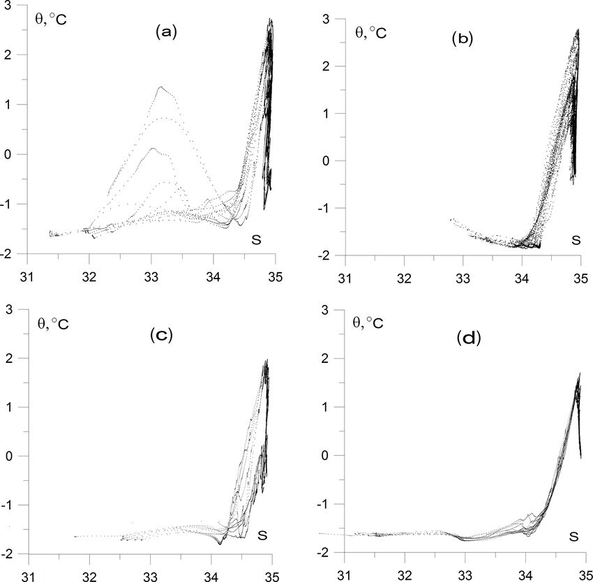
412              N. Zhurbas and N. Kuzmina: Variability of the thermohaline structure and transport of Atlantic water

Figure 7. θ –S diagrams based on the CTD profiling in (a) the St. Anna Trough (NABOS09, 82◦ N), (b) the PS96 section at 92◦ E, and the
NABOS09 sections at 103◦ E (c) and 142◦ E (d). For convenience of presentation, the points of the θ –S curves with salinity below 30 were
excluded.

the slope of the Nansen Basin (see Fig. 4). Curve 6 corre-             BSBW mode. To evaluate the transformation of the “true”
sponds to the UPDW. The θ –S diagrams for CTD profiles in              mode of BSBW an additional analysis is required, which is
the section 103◦ E are presented by curves 8–11 (see Fig. 5            beyond the scope of this paper.
for the locations of stations). Curves 8, 9, and 10 are simi-             The BSBW, which is characterized by the knee-shape di-
lar to curve 2 and indicate the BSBW. Curve 11, similar to             agram in coordinates θ –S and σθ –S, is not visible at 126◦ E
curve 6 in Fig. 8c, corresponds to the UPDW. However, the              (Fig. 8). This is consistent with the conclusion formulated in
BSBW is not observed at 126◦ E: see Fig. 8e, where a col-              Sect. 3.1.1 that by 126◦ E the BSBW is not accompanied by
lection of θ –S curves (collectively referred as 12) presents          any noticeable tilt of isopycnals. Moreover, given the char-
all CTD profiles in the depth range 500–1800 m measured at             acteristic feature of the θ –S structure of BSBW in the St.
126◦ E of NABOS09. Also, we do not observe the BSBW                    Anna Trough (curves 1–4 in Fig. 8a) was observed in other
further to the east on the 142◦ E section of NABOS09 (not              years, we carried out a similar analysis using all available
shown) or in the Makarov Basin.                                        CTD data and found that the BSBW is not distinct at this
   The BSBW at 103◦ E is also characterized by a knee shape            longitude (see Fig. 9). The only exception was 2002, when
in σθ and S coordinates (Fig. 8f, numbers correspond to those          the BSBW was still observed at 126◦ E. It suggests that the
in other panels). However the knee-shape diagram is not ob-            BSBW and FSBW begin to mix intensively immediately af-
served along 126◦ E (curves 12) in these coordinates. The              ter 103◦ E. On the other hand, the FSBW is well identified
dense and cold deep waters in the section 126◦ E have σθ , θ ,         at 126◦ E and further along the slope of the Eurasian Basin
and S values typical for the “true” BSBW mode (Dmitrenko               (and even in the Makarov Basin), while we cannot say the
et al., 2015). Nevertheless, these waters (see σθ and S values         same about the BSBW. Thus, one may assume that east of
inside the circle; Fig. 8f) also correspond to the UPDW char-          126◦ E the geostrophic volume flow rate of the AW is mainly
acteristics and hence cannot be distinguished as the “true”            provided by the FSBW.

Ocean Sci., 16, 405–421, 2020                                                                       www.ocean-sci.net/16/405/2020/
N. Zhurbas and N. Kuzmina: Variability of the thermohaline structure and transport of Atlantic water                                          413

Figure 8. Thermohaline values of the BSBW and FSBW. (a) Based upon the CTD profiles, obtained in the St. Anna Trough (NABOS09,
section 82◦ N); curves 1–4 correspond to the stations (st.) 76, 78, 83, and 80, respectively. (b) The same as (a) but only curves 1 and 2 are
presented; regions I, II, III illustrate three different water masses in accordance with Dmitrenko et al. (2015); for an explanation, see the text.
(c) Based upon the section of PS96, curves 5 and 6 corresponding to st. 32 and 42, respectively (depth range 600–1000 m), curves 2 and
3 are shown for the reference. (d) For CTD profiles in the 103◦ E section, NABOS09, curve 8 (st. 64), curve 9 (st. 63), curve 10 (st. 62),
curve 11 (st. 60), and curve 2 for the reference (see Fig. 5 for the location of the stations). (e) Based upon the CTD profiles in the depth range
500–1200 m measured at 126◦ E (section of NABOS09), curves 12; curves 2, 9, and 10 are shown for the reference. (f) The same as (e) but
presented in coordinates σθ and S.

www.ocean-sci.net/16/405/2020/                                                                                Ocean Sci., 16, 405–421, 2020
414              N. Zhurbas and N. Kuzmina: Variability of the thermohaline structure and transport of Atlantic water

Figure 9. θ –S diagrams based on the CTD profiling: NABOS05 – (a, b), 103◦ E (a), 126◦ E (b); NABOS06 – (c, d), 103◦ E (c), 126◦ E (d);
NABOS08 – (e, f), 103◦ E (e), 126◦ E (f).

3.2   Characteristics of the Atlantic water flow and                  are presented in Table 2. The only exception is the transect
      geostrophic estimates of the volume flow rate                   at 82◦ N, where the near-bottom gravity current with a con-
                                                                      siderable eastward component due to overflow across a suf-
The estimates of the geostrophic volume flow rate and                 ficiently deep ridge (≈ 500 m deep) east of the St. Anna
the hydrological parameters describing the AW flow in the             Trough (Fig. 3a–c) makes the estimate of AW transport
Eurasian and Makarov basins are presented in Table 1. The             northward questionable. Note also that to the west of the St.
geostrophic estimates of the near-bottom volume flow rate             Anna Trough our estimates refer to the FSBW; to the east
of the BSBW in zonal transects across the St. Anna Trough             of this region BSBW enters the Eurasian Basin and our esti-

Ocean Sci., 16, 405–421, 2020                                                                      www.ocean-sci.net/16/405/2020/
N. Zhurbas and N. Kuzmina: Variability of the thermohaline structure and transport of Atlantic water 415 mates should be attributed to the joint contribution of the two rate values averaged is N = 6). Similarly, the average volume branches (FSBW and BSBW). flow rate was calculated for the region 94–107◦ E (region II; The hydrological parameters shown in Table 1 can be in- N = 9). The remaining average estimates of geostrophic vol- terpreted as follows. The maximum water temperature of the ume flow rate were calculated for sections 126◦ E (region III; AW may exceed 5 ◦ C in cases when the AW inflow to the N = 9), 142◦ E (region IV; N = 10), and 159◦ E (region V; Eurasian Basin consists of especially warm water masses. N = 2). Then the 95 % and 80 % confidence intervals were Typical changes in the temperature and salinity maxima of determined using the Student t distribution. All estimates of the AW moving along the slope over a distance of about average volume flow rates and confidence intervals are pre- 1000 km are approximately 1–2 ◦ C and 0.1, respectively. sented in Tables 1 and 2. These changes lead to a slight increase in potential density, On average, the volume flow rate increases from region and therefore a deviation of the AW from the isopycnic distri- I to region II and then decreases to region III and region bution can be expected. These changes are most likely asso- IV, followed by a sharp decrease in region V. However, only ciated with the exchange of heat, salt, and mass with the sur- the difference between the volume flow rate in region II and rounding waters through intrusive layering and double dif- the values in regions IV and V are significant at 95 % confi- fusion (see, e.g., Kuzmina et al., 2011, 2018; Polyakov et dence. Transport values bounded by the confidence intervals al., 2012) and sea ice melting and cooling (Rudels, 1998). for regions II, IV, and V are (0.46; 1.72), (0.12; 0.44), and The intrusions, in particular, can also contribute to the reduc- (−0.37; 0.43), respectively. These intervals indicate that the tion in the AW heat and salt content and the volume flow mean volume flow rate in region II exceeds the value of the rate. The differences in the AW heat and salt content and the same parameter in regions IV and V with a high probability volume flow rate can be clearly seen from the PS96 section of 95 %. The 80 % confidence intervals overlap only for re- when comparing data from stations near the continental slope gions III and IV: (0.25; 0.53) and (0.18; 0.38), respectively. In of the Eurasian Basin at 92◦ E and from the vicinity of the this regard, the change in the volume flow rate along the slope Lomonosov Ridge at 140◦ E. is significant with a probability of 80 %, except for changes It is worth noting that the maximum value of the AW tem- in volume flow rate from region III to region IV. perature (θmax ) in this data set is always observed in the upper The above values of the mean volume flow rate and confi- layer of the Eurasian Basin at depths below the pycnocline dence intervals also suggest that the increase in volume flow but not exceeding 350 m, while the maximum salinity (Smax ) rate in 2006 is significant and not caused by the “noise” in at sections in the eastern part of the basin can be observed at the data. Indeed, the volume flow rates in regions II, III, and depths greater than 1000 m. IV in 2006 exceeded the upper limits of the corresponding Xθmax in Table 1 is the distance of the AW core (which can 95 % confidence intervals. From a statistical point of view be associated with θmax ) from the slope–shelf boundary. The such a significant increase in volume flow rates at the same highest value and the maximum variation in this parameter time in three regions is a very rare event that can hardly be are observed near 126 and 142◦ E, where a two-core structure explained by random “noise” in the data caused, for example, of AW is often observed (Pnyushkov et al., 2015). by the influence of synoptic eddies. The noticeable increase in θmax in 2006 at 31 and 103◦ E Let us turn our attention to the following features of the and the intensive warming of the AW were first reported in volume flow rate estimates: high volume flow rate estimates Polyakov et. al. (2011). The present results show that the in- at 96, 103, and 107◦ E, a negative volume flow rate estimate crease in the temperature of the AW in 2006 was also ac- at 126◦ E in 2013, and low volume flow rate estimates at 31 companied by an increase in volume transport (see Table 1, and 98◦ E in 2009 (Table 1). Indeed, the AW volume flow rate the section along 103◦ E, and reasonings below). This can be in the BSBW area of entry into the Eurasian Basin in 2013 caused not only by the warming of the AW but also by an was almost equal to the maximum volume flow rate in 2006 increased inflow of the AW to the Eurasian Basin. (103◦ E) and was quite high, up to the longitude 107◦ E. This The geostrophic transport in the range of 31–159◦ E is phenomenon as well as the intense warming in 2006 can be characterized by a high variability (Table 1). This may be associated with the recent changing conditions in the Arctic. due to (a) a section orientation oblique to the current; (b) We hypothesize that the negative volume flow rate at 126◦ E the difference in the horizontal scales of the sections; (c) un- was because of the influence of local return flows which can certainty in the choice of the reference level for geostrophic be observed near the slope (Pnyushkov et al., 2015). Low calculations; (d) meandering of the flow; and (e) the effect of FSBW volume flow rate estimates in 2009 are probably as- synoptic quasi-geostrophic eddies on the flow volume rate. sociated with a strong deviation of the flow from the slope, In order to find statistically consistent estimates of the vari- which may underestimate the AW volume transport due to ability of geostrophic volume flow rate along the slope of the the small length of the transects to the north (see also Sect. 4). basin based on a limited data set, the following was done. The mean value of the FSBW volume flow rate in re- The volume flow rates obtained for all sections within the gion I is Vmean = 0.5 Sv. This estimate of volume flow rate range 31–92◦ E for different years were used to calculate the is about half the estimate of the BSBW mean volume flow mean volume flow rate (region I; the number of volume flow rate: Vmean = 0.79 Sv (N = 3, Table 2). (The difference is www.ocean-sci.net/16/405/2020/ Ocean Sci., 16, 405–421, 2020
416               N. Zhurbas and N. Kuzmina: Variability of the thermohaline structure and transport of Atlantic water

Table 1. Characteristics of the Atlantic water flow in the course of its propagation along a continental slope of the Eurasian Basin of the
Arctic Ocean. “Dist” is the along-slope distance from Fram Strait; θmax is the maximum temperature; σθ (Zθmax ), S(Zθmax ), Zθmax , and
Xθmax are the values of potential density, salinity, depth, and lateral displacement from the slope for the point θmax ; Smax and ZSmax are the
maximum salinity and depth of Smax ; V is the geostrophic estimate of the volume flow rate. The mean values, 95 % confidence intervals, and
80 % confidence intervals of the volume flow rate, Vmean , calculated separately for CTD transects at 31–92, 94–107, 126, 142, and 159◦ E,
are also shown. The last row in the Table presents the characteristics of the return flow of the AW by the Lomonosov Ridge at 140◦ E and
86.5◦ N (PS96; see Fig. 1).

           Exp                   Long     Dist     θmax    σθ (Zθmax )   S(Zθmax )    Zθmax    Xθmax       Smax    ZSmax         V
                                 (◦ E)   (km)      (◦ C)    (kg m−3 )                   (m)     (km)                 (m)       (Sv)
           NABOS06                 31     404     5.670        27.579      34.980        42      −11     35.099        72      0.57
           NABOS08                 31     404     4.883        27.771      35.103       101        0     35.105       176      0.80
           NABOS09                 31     404     3.691        27.818      34.999        89        0     35.002        91      0.10
           NABOS09                 60     856     2.503        27.891      34.951       175       10     34.981       363      0.47
           NABOS13                 90    1290     2.600        27.903      34.975       250       41     34.996       333      0.46
           PS96                    92    1322     2.786        27.875      34.960       271       33     34.968       329      0.58
           Vmean = 0.50 ± 0.24/ ± 0.14 Sv
           NABOS15                 94    1355     2.445        27.946      35.012       331        33    35.015       365      0.47
           NABOS13                 96    1388     2.548        27.902      34.969       207        70    34.978       264      2.06
           NABOS09                 98    1421     2.300        27.906      34.948       220        79    34.971       345      0.09
           NABOS05                103    1561     2.029        27.870      34.876       179        39    34.934       309      0.32
           NABOS06                103    1561     2.528        27.888      34.950       220        50    34,978       260      2.23
           NABOS08                103    1561     1.980        27.886      34.891       201        60    34.929       325      0.42
           NABOS09                103    1561     1.984        27.913      34.925       244        50    34.951       365      0.87
           NABOS13                103    1561     2.278        27.904      34.942       215        80    34.956       419      1.59
           NABOS13                107    1695     1.903        27.937      34.945       359       120    34.948       404      1.77
           Vmean = 1.09 ± 0.63/ ± 0.38 Sv
           NABOS02                126    2104     1.406        27.938      34.902       324       243    34.932     2061      0.05
           NABOS03                126    2102     1.341        27.941      34.899       336       342    34.921     1886      0.41
           NABOS04                126    2102     1.770        27.906      34.896       271        87    34.925     2431      0.61
           NABOS05                126    2102     1.695        27.936      34.926       359       227    34.935     2841      0.75
           NABOS06                126    2102     1.905        27.923      34.930       284       193    34.960      968      0.77
           NABOS07                126    2102     2.085        27.907      34.928       266       242    34.942      340      0.60
           NABOS08                126    2102     2.195        27.885      34.911       206       235    34.939      365      0.31
           NABOS09                126    2102     1.907        27.909      34.913       316        33    34.932     1018      0.40
           NABOS13                126    2102     1.946        27.937      34.949       346       228    34.951      428     −0.21
           NABOS15                126    2102     1.653        27.918      34.898       246       400    34.942     3816      0.22
           Vmean = 0.39 ± 0.22/ ± 0.14 Sv
           NABOS03                142    2456     1.089        27.912      34.841       269        41    34.862     1000       0.06
           NABOS04                142    2456     1.401        27.909      34.865       281         0    34.907     1608       0.21
           NABOS05                142    2456     1.492        27.906      34.870       284       100    34.906     1550       0.26
           NABOS06                142    2456     1.981        27.874      34.876       234       111    34.960     1016       0.60
           NABOS07                142    2456     1.855        27.879      34.870       231         0    34.920     2064       0.09
           NABOS08                142    2456     1.599        27.915      34.890       260       200    34.908      347       0.23
           NABOS09                142    2456     1.704        27.915      34.900       253       101    34.917     1082       0.22
           NABOS13                142    2456     1.475        27.940      34.909       331       115    34.926     1150       0.18
           NABOS15                142    2456     1.353        27.936      34.892       326       106    34.913     1372       0.63
           Vmean = 0.28 ± 0.16/ ± 0.10 Sv
           NABOS07                159    2783     1.424        27.887      34.839       255         0    34.880     1075     −0.01
           NABOS08                159    2783     1.383        27.893      34.843       245         0    34.889     1266      0.06
           Vmean = 0.03 ± 0.40/ ± 0.10 Sv
           PS96          140E 86.5 N     3178     1.812        27.890      34.880       219    ≈ 700     34.902       472    −0.09

Ocean Sci., 16, 405–421, 2020                                                                           www.ocean-sci.net/16/405/2020/
N. Zhurbas and N. Kuzmina: Variability of the thermohaline structure and transport of Atlantic water 417
Table 2. Geostrophic estimates of the volume flow rate for near-
bottom gravity flow of the Barents Sea branch of Atlantic water
(BSBW) on zonal transects across the St. Anna Trough. The uncer-
tainty estimates are 95 % and 80 % confidence intervals.
Exp NABOS09 NABOS13 NABOS15
Lat (◦ N) 81.00 81.33 81.41 Vmean
V (Sv) 0.89 0.73 0.76 0.79 ± 0.22/ ± 0.10
significant at 80 % confidence interval.) The BSBW mean
volume flow rate exceeding nearly twice the FSBW mean
volume flow rate results in a dominance of the BSBW pat-
tern of potential density contours in the longitude range
of 94–107◦ E (region II), where both branches of the AW
are present. Moreover, the sum of the mean values of the
FSBW and the BSBW geostrophic volume flow rate es-
timates Vmean = 0.5 + 0.79 = 1.29 Sv corresponds well to
the combined FSBW and BSBW flow within the region II:
Vmean = 1.09 Sv. Thus, the increase in geostrophic volume
transport in region II is mainly due to the influence of the
BSBW. The decrease in geostrophic volume transport in re-
gion III can also be associated primarily with the BSBW,
namely, with the decrease in the BSBW volume transport in
the 126◦ E section and further along the slope (see Sect. 3.1.1
and 3.1.2).
Finally, at the 159◦ E section in the Makarov Basin, the
geostrophic estimate of the along-slope volume flow rate of
mixed waters of the FSBW and the BSBW has further greatly
reduced down to Vmean = 0.03 Sv (N = 2), which is more
than 1 order of magnitude smaller than that in the Nansen and
Amundsen basins. Despite the low statistical significance of
the latter estimate (due to the small value of N = 2) one may
conclude that the major part of the AW entering the Arctic Figure 10. Interannual variability of the maximum temperature
Ocean circulates cyclonically within the Nansen and Amund- θmax and the related values of salinity S(θmax ), potential density
sen basins, and only its small part flows to the Makarov anomaly σθ (θmax ), and volume flow rate V on the cross-slope tran-
Basin (Rudels et al., 2015; Rudels, 2015). However, addi- sects at 103, 126, and 142◦ E.
tional studies are required to confirm this result.
3.3 Interannual variability of the AW
temperature–salinity values and the volume flow this period was as large as 0.6–1.0 ◦ C relative to 2002–2003
rate and 0.3–0.6 ◦ C relative to 2013–2015. In 2006, S(θmax ) dis-
played local maxima at the transects 126 and 142◦ E and the
Within the NABOS project, the cross-slope CTD transects at absolute maximum at the transect 103◦ E; the salinity excess
103, 126, and 142◦ E were repeatedly performed for a num- for the maxima largely decreased with the longitude from ap-
ber of annual campaigns (Table 1): 2005, 2006, 2008, and proximately 0.06 at 103◦ E to less than 0.01 at 142◦ E. θmax
2013 (103◦ E); 2002–2009, 2013, and 2015 (126◦ E); 2003– had a maximum in 2013 but only at 103◦ E (see Table 1 and
2009, 2013, and 2015 (142◦ E). We use the repeated transects Fig. 10). The time series of S(θmax ) display a trend of in-
to describe the interannual variability of the AW. crease in AW salinity over time, which can be referred to as
Time series of the AW temperature maximum, θmax , and an AW salinization in the early 2000s. The salinity of AW
the related values of salinity S(θmax ) and potential density at 142◦ E increases almost monotonously in the period from
anomaly σθ (θmax ) (Fig. 10) show that the period of 2006 to 2003 to 2013. The mechanism behind this salinity evolution
2008 was characterized by an increased temperature of the is not clear. It is also worth noting that the maxima of θmax
AW in the eastern part of the Eurasian Basin, an increased and S(θmax ) in 2006 and 2013 (at 103◦ E) were accompanied
salinity and density reduction. The temperature excess during by maxima in transport.
www.ocean-sci.net/16/405/2020/ Ocean Sci., 16, 405–421, 2020418 N. Zhurbas and N. Kuzmina: Variability of the thermohaline structure and transport of Atlantic water
4 Discussion mates. However, the upper confidence limit of our es-
timate does not reach 1 Sv. Moreover, we used T >
Here we discuss the following issues: (a) differences in 0 ◦ C to identify the AW, while in Beszczynska-Möller
the identification of the BSBW; (b) a comparison of the et al. (2012) the volume flow rates of the AW entering
geostrophic volume flow rate estimates with other studies; the Eurasian Basin through Fram Strait were determined
(c) the weakening of the BSBW signal at 126◦ E and further for waters with T > 2 ◦ C. Comparatively smaller trans-
east. port in region I may be because the sections along 31◦ E
a. Advection and interaction of waters with different θ –S (see Fig. 1) are less than 100 km wide and do not cover
characteristics in the Arctic Basin, as well as the impact the full extent of the FSBW (Fig. 2). Given the sensi-
of climate change that has been observed over the past tivity to the definition of AW and the resulting cross-
decade (Polyakov et al., 2017) complicate an accurate sectional area (see point “a” above), the volume trans-
identification of water masses. However, a robust ap- port may be underestimated. It is possible that the for-
proach proposed in Dmitrenko et al. (2015) is effective mation and passage of synoptic eddies leads to variabil-
for distinguishing the water masses of the FSBW and ity in volume transports. According to Perez-Hernandez
BSBW branches. As an exception, this approach fails et al. (2017) north of Svalbard (between 21 and 33◦ E)
when the FSBW temperature is below 0 ◦ C (see Fig. 2 in September 2013, a large difference was found in the
in Dmitrenko et al., 2015) and/or the BSBW tempera- estimates of geostrophic volume flow rate (from 0.53 to
ture is close to 1 ◦ C (see Fig. 6 in Schauer et al., 2002a). 3.39 Sv) due to the passage of eddies and meandering
If such cases are rare, then either of the two approaches of the current. Våge et al. (2016) based on geostrophic
can be used to identify the BSBW and FSBW. Indeed, velocities at two CTD sections across the boundary cur-
the identification of the BSBW on the PS96 section in rent near 30◦ E (September 2012) evaluated a net AW
our case (we used the approach proposed by Dmitrenko volume flow rate of 1.6 ± 0.3 Sv. They found evidence
et al., 2015; see Sect. 3.1.1) does not differ much from of a large eddy affecting the mean volume transport cal-
that proposed by Schauer et al. (2002b). However, these culations. The barotropic velocity component, which is
discrepancies can lead to almost an order of magnitude not taken into account in our estimates, can also con-
difference in estimates of the volume flow rate of the tribute to larger transports. However, in conditions with
BSBW only due to the differences in the BSBW cross- high ice concentration in the Eurasian Basin, we might
sectional area. expect a reduced barotropic contribution from the sea
level changes induced by wind forcing. In cruise re-
b. Based on the velocity measurements with moored in- ports, the NABOS CTD sections were characterized by
struments (1997–2010) in the area of the West Spitsber- ice concentrations of 50 %–100 % (see https://uaf-iarc.
gen Current (WSC) near Fram Strait (zonal transect at org/nabos-cruises/, last access: 3 May 2019, IARC,
∼78◦ 500 N) , approximately 3 Sv of the AW flows into 2019). Exceptions occurred in the near-slope areas of
the Nansen Basin (Beszczynska-Möller et. al., 2012). the Laptev Sea, that is, in the sections along ∼ 126◦ E,
The long-term mean volume transport confined to the where the ice concentration varied from 0 % to 100 %,
WSC core branch (or Svalbard branch in accordance having a maximum value in the northern part of the sec-
with Schauer et al., 2004) included 1.3 ± 0.1 Sv of tions. In such areas, the contribution of the barotropic
the AW warmer than 2 ◦ C. The offshore WSC branch component to the flow velocity can be large. For exam-
(or Yermak branch) carried on average 1.7 ± 0.1 Sv of ple, using long-term measurements (1995–1996) from
the AW. The variability range of the AW geostrophic a mooring in the near-slope area of the Laptev Sea,
transport of the Svalbard branch for meridional sec- Woodgate et al. (2001) showed that the contribution of
tions from 1997, 2001, and 2003 (summer and fall) the barotropic component to the velocity of the Arctic
was between 0.06 and 0.7 Sv (Marnela et al., 2013). In Ocean boundary current (AOBC) was equal to the con-
Kolås and Fer (2018) observations of the oceanic cur- tribution of the first three baroclinic modes. Assuming
rent and thermohaline field (in summer 2015) in the an average velocity based on the measurements in the
three sections were used to characterize the evolution upper 1200 m layer of 4.5 cm s−1 and a width of 50 to
of the WSC along 170 km downstream distance. Abso- 84 km the volume flow rate was estimated at 5 ± 1 Sv.
lute geostrophic transports of AW ranged from 0.6 to This is larger than our average estimate of the AW vol-
1.3 Sv in the Svalbard branch. In accordance with ear- ume flow rate along 126◦ E (0.39 ± 0.22, Table 1) by an
lier studies of the currents in Fram Strait, recirculation order of magnitude. Such a difference can be explained
of the AW can be significant, and the volume flow rate not only by the absence of a barotropic contribution in
of the AW entering the Arctic Ocean ranges from 0.6 to our case, but also by the fact that we took into account
1.5 Sv (Rudels, 1987; Aagaard and Carmack, 1989). the volume transport of AW only (i.e., the cold, low-
Our estimate of the mean volume flow rate Vmean in salinity surface layer was excluded) and considered a
region I (31–92◦ E) is in the range of the above esti- certain season (August and September). Indeed, accord-
Ocean Sci., 16, 405–421, 2020 www.ocean-sci.net/16/405/2020/N. Zhurbas and N. Kuzmina: Variability of the thermohaline structure and transport of Atlantic water 419
ing to long-term measurements at six moorings on a sec- 5 Summary
tion along 126◦ E, the AOBC volume flow rate varied
from 0.3 to 9 Sv (Pnyushkov et al., 2018b). Such a wide
range in volume flow rate estimates is probably due to The θ–S properties and the volume flow rate estimates of the
a combined effect of seasonal variability and mesoscale current carrying the AW in the Eurasian Basin and St. Anna
eddies (Pnyushkov et al., 2018a). Trough were obtained based on the analysis of CTD data col-
lected within the NABOS program in 2002–2015; addition-
The fact that seasonal variations can in some cases ally CTD transect PS96 was considered.
significantly affect the AW volume flow rates (see FSBW was present at all transects, including the two tran-
also the discussion in Pnyushkov et al., 2018b) is sects in the Makarov Basin (159◦ E), while the cold waters
confirmed by a number of observations (Schauer et at the transects along longitudes 126, 142, and 159◦ E, which
al., 2002a; Beszczynska-Möller et al., 2012; Pnyushkov can be associated with the influence of the BSBW, were ob-
et al., 2018b). For example, the volume flow rate of the served in the depth range below 800 m and had little effect on
AW in the northwestern part of the Barents Sea was the spatial structure of isopycnic surfaces and the horizontal
0.6 Sv (Schauer et al., 2002a). This agrees well with our gradient of density. It is shown using θ —S analysis that the
estimate of the AW transport in the St. Anna Trough BSBW signal, which is characterized by the knee-shape fea-
of 0.79 ± 0.22 Sv (Table 2). However, the analysis of ture in coordinates θ and S and σθ and S (see Fig. 8), is either
current velocity measurements in the winter season at strongly weakened or not visible at the longitude 126◦ E (ex-
the same section in the northwestern part of the Barents cluding the observations in 2002 at 126◦ E), while the FSBW
Sea gave a completely different estimate of ∼ 2.6 Sv signal is well identified at 126◦ E and further along the slope
(Schauer et al., 2002a). of the Eurasian Basin. Based on the revealed features of the
c. According to Dmitrenko et al. (2009), the BSBW can temperature, salinity, and density fields, it is suggested that
be satisfactorily identified at 142◦ E. However, a “pat- east of 126◦ E the geostrophic volume transport of AW is
tern” in the θ –S diagram far from the place of the mainly provided by the FSBW.
BSBW entry into the Eurasian Basin can be regarded The geostrophic volume transport of AW increases (with
as the BSBW signal if it maintains the similarity with 80 % confidence) from the region of 31–92◦ E (0.5±0.14 Sv)
the “pattern” of the BSBW at the exit from the St. Anna to the region of 94–107◦ E (1.09 ± 0.38 Sv) and then de-
Trough, that is, with the so-called “knee” (Dmitrenko creases to the region of 126◦ E (0.39 ± 0.14 Sv) and becomes
et al., 2015). Our analysis showed that the “knee” is small (0.03 ± 0.1 Sv) in the Makarov Basin (159◦ E).
regularly observed at 103◦ E, while at 126◦ E it is ab- The temporal variability of hydrological parameters and of
sent, weak, or distorted. This may be expected since the AW volume flow rate is summarized as follows. The time
the flow velocity is small and the BSBW covers a dis- series of θmax had an absolute maximum in 2006–2008 that
tance from 103 to 126◦ E for 1–2 years. However, de- can be interpreted as a result of heat pulse in the early 2000s
(Polyakov et al., 2011). In accordance with our analysis the
spite such a long travel time, Fram Strait branch is
well identified not only at 126◦ E but also further along time series of θmax had a maximum in 2013 but only at the
the slope. This suggests stronger transformation and longitude 103◦ E (Table 1 and Fig. 10). The time series of
mixing of, primarily, the BSBW. The BSBW transfor- S(θmax ) display a trend of increase in AW salinity over time,
mation can be due to various reasons, including mix- which can be referred to as an AW salinization in the early
ing with the FSBW caused by thermohaline intrusive 2000s. Moreover the salinity increases almost monotonously
layering at absolutely stable stratification (Merryfield, in the period from 2003 to 2013 at 142◦ E. It is important to
2002; Kuzmina et al., 2014; Kuzmina, 2016), the influ- underline also that the maxima of θmax and S(θmax ) in 2006
ence of the slope topography, the impact of local coun- and 2013 (103◦ E) are accompanied by the volume flow rate
terflows near the slope (see, for example, Pnyushkov highs. A significant increase in geostrophic volume flow rate
et al., 2015), lateral convection (Ivanov and Shapiro, identified in 2006 is likely associated with the recent change
2005; Ivanov and Golovin, 2007; Walsh et al., 2007), observed in the Arctic Ocean.
the impact of the Arctic Shelf Break Water (Aksenov et
al., 2011; Ivanov and Aksenov, 2013), and mixing due
Data availability. All CTD data used in this paper can be accessed
to eddies (Schauer et al., 2002; Dmitrenko et al., 2008;
from the NABOS project website http://nabos.iarc.uaf.edu (last ac-
Aagaard et al., 2008; Pnyushkov et al., 2018a). The un- cess: 24 January 2019, IARC, 2019).
derstanding of the processes of transformation and mix-
ing of the BSBW and FSBW is necessary to verify an
important concept proposed by Rudels et al. (2015) that Author contributions. NZ proposed the idea of research, developed
the BSBW supplies the major part of the AW to the approaches to data processing, estimated the transports and aver-
Amundsen, Makarov, and Canadian basins, while the age thermohaline characteristics of Atlantic waters, and described
FSBW remains almost fully in the Nansen Basin. results. NK carried out θ –S analysis and statistical analysis. Both
www.ocean-sci.net/16/405/2020/ Ocean Sci., 16, 405–421, 2020420 N. Zhurbas and N. Kuzmina: Variability of the thermohaline structure and transport of Atlantic water
authors contributed to the interpretation of the results and writing Kaleschke, L., Bauch, D., Hölemann, J. A., and Timo-
the paper. khov, L. A.: Seasonal modification of the Arctic Ocean in-
termediate water layer off the eastern Laptev Sea conti-
nental shelf break, J. Geophys. Res.-Oceans, 114, C06010,
Competing interests. The authors declare that they have no conflict https://doi.org/10.1029/2008JC005229, 2009.
of interest. Dmitrenko, I. A., Rudels, B., Kirillov, S. A., Aksenov, Y. O.,
Lien V. S., Ivanov, V. V., Schauer, U., Polyakov, I. V., Cow-
ard, A., and Barber, D. J.: Atlantic Water flow into the
Acknowledgements. This research, including the approach devel- Arctic Ocean through the St. Anna Trough in the north-
opment, data processing, and interpretation, performed by Nataliya ern Kara Sea, J. Geophys. Res.-Oceans, 120, 5158–5178,
Zhurbas, was funded by Russian Science Foundation (project no. https://doi.org/10.1002/2015JC010804, 2015.
17-77-10080). Natalia Kuzmina (θ –S analysis, statistical analysis, IARC: Nansen and Amundsen Basins Observational System NA-
participation in discussion) was supported by the state assignment BOS, available at: http://nabos.iarc.uaf.edu, last access: 24 Jan-
of the Shirshov Institute of Oceanology RAS (theme no. 0149- uary 2019.
2019-0003). Ivanov, V. and Golovin, P.: Observations and modelling of dense
The authors are very grateful to the NABOS group for providing water cascading from northwestern Laptev Sea shelf, J. Geophys.
the opportunity to use the CTD data. Res., 112, C09003, https://doi.org/10.1029/2006JC003882,
The authors are very grateful to the editor for evaluating the arti- 2007.
cle and help in the work on the text and to the anonymous reviewers Ivanov, V. V. and Aksenov, E. O.: Atlantic Water transformation
for useful comments. in the Eastern Nansen Basin: observations and modelling, Arct.
Antarct. Res., 1, 72–87, 2013 (in Russian).
Ivanov, V. V. and Shapiro, G. I.: Formation of dense water cascade
in the marginal ice zone in the Barents Sea, Deep-Sea Res. Pt. I,
Financial support. This research was funded by Russian Science
52, 1699–1717, https://doi.org/10.1016/j.dsr.2005.04.004, 2005.
Foundation (project no. 17-77-10080) and by the state assignment
Kolås, E. and Fer, I.: Hydrography, transport and mixing of the
of the Shirshov Institute of Oceanology RAS (theme no. 0149-
West Spitsbergen Current: the Svalbard Branch in summer 2015,
2019-0003).
Ocean Sci., 14, 1603–1618, https://doi.org/10.5194/os-14-1603-
2018, 2018.
Kuzmina, N.: Generation of large-scale intrusions at baroclinic
Review statement. This paper was edited by Ilker Fer and reviewed fronts: an analytical consideration with a reference to the Arctic
by two anonymous referees. Ocean, Ocean Sci., 12, 1269–1277, https://doi.org/10.5194/os-
12-1269-2016, 2016.
Kuzmina, N., Rudels, B., Zhurbas, V., and Stipa, T.: On the struc-
ture and dynamical features of intrusive layering in the Eurasian
References Basin in the Arctic Ocean, J. Geophys. Res., 116, C00D11,
https://doi.org/10.1029/2010JC006920, 2011.
Aagaard, K.: On the deep circulation of the Arctic Ocean, Deep-Sea Kuzmina, N. P., Zhurbas, N. V., Emelianov, M. V., and Pyzhe-
Res., 28, 251–268, 1981. vich, M. L.: Application of interleaving Models for the De-
Aagaard, K. and Carmack, E. C.: The role of sea ice and other fresh scription of intrusive Layering at the Fronts of Deep Polar Wa-
water in the Arctic circulation, J. Geophys. Res., 94, 14485– ter in the Eurasian Basin (Arctic), Oceanology, 54, 557–566,
14498, https://doi.org/10.1029/JC094iC10p14485, 1989. https://doi.org/10.1134/S0001437014050105, 2014.
Aagaard, K., Andersen, R., Swift, J., and Johnson, J.: A large eddy Kuzmina, N. P., Skorokhodov, S. L., Zhurbas, N. V., and
in the central Arctic Ocean, Geophys. Res. Lett., 35, L09601, Lyzhkov, D. A.: On instability of geostrophic current with linear
https://doi.org/10.1029/2008GL033461, 2008. vertical shear at length scales of interleaving, Izv. Atmos. Ocean.
Aksenov, Y., Ivanov, V. V., Nurser, A. J. G., Bacon, S., Phys., 54, 47–55, https://doi.org/10.1134/S0001433818010097,
Polyakov, I. V., Coward, A. C., Naveira-Garabato, A. C., 2018.
and Beszczynska-Moeller, A.: The Arctic Circumpolar Marnela, M., Rudels, B., Houssais, M.-N., Beszczynska-Möller, A.,
Boundary Current, J. Geophys. Res., 116, C09017, 1–28, and Eriksson, P. B.: Recirculation in the Fram Strait and trans-
https://doi.org/10.1029/2010JC006637, 2011. ports of water in and north of the Fram Strait derived from CTD
Beszczynska-Möller, A., Fahrbach, E., Schauer, U., and Hansen, E.: data, Ocean Sci., 9, 499–519, https://doi.org/10.5194/os-9-499-
Variability in Atlantic water temperature and transport at the en- 2013, 2013.
trance to the Arctic Ocean, 1997–2010, ICES J. Mar. Sci., 69, Merryfield, W. J.: Intrusions in Double-Diffusively Stable Arctic
852–863, https://doi.org/10.1093/icesjms/fss056, 2012. Waters: Evidence for Differential mixing?, J. Phys. Oceanogr.,
Dmitrenko, I. A., Kirillov, S. A., Ivanov, V. I., and Woodgate, R.: 32, 1452–1459, 2002.
Mesoscale Atlantic water eddy off the Laptev Sea continental Pérez-Hernández, M. D., Pickart, R. S., Pavlov, V., Våge, K., Ing-
slope carries the signature of upstream interaction, J. Geophys. valdsen, R., Sundfjord, A., Renner, A. H. H., Torres, D. J., and
Res., 113, C07005, https://doi.org/10.1029/2007JC004491, Erofeeva, S. Y.: The Atlantic Water boundary current north of
2008. Svalbard in late summer, J. Geophys. Res.-Oceans, 122, 2269–
Dmitrenko, I. A., Kirillov, S. A., Ivanov, V. V., Woodgate, R. A., 2290, https://doi.org/10.1002/2016JC012486, 2017.
Polyakov, I. V., Koldunov, N., Fortier, L., Lalande, C.,
Ocean Sci., 16, 405–421, 2020 www.ocean-sci.net/16/405/2020/You can also read