Implicit Semi-Algebraic Abstraction for Polynomial Dynamical Systems
←
→
Page content transcription
If your browser does not render page correctly, please read the page content below
Implicit Semi-Algebraic Abstraction
             for Polynomial Dynamical Systems

    Sergio Mover1 , Alessandro Cimatti2 , Alberto Griggio2 , Ahmed Irfan3 , and
                                Stefano Tonetta2
            1
                Ecole Polytechnique, LIX, Institut Polytechnique de Paris
                             2
                               Fondazione Bruno Kessler
                                3
                                  Stanford University

       Abstract. Semi-algebraic abstraction is an approach to the safety veri-
       fication problem for polynomial dynamical systems where the state space
       is partitioned according to the sign of a set of polynomials. Similarly to
       predicate abstraction for discrete systems, the number of abstract states
       is exponential in the number of polynomials. Hence, semi-algebraic ab-
       straction is expensive to explicitly compute and then analyze (e.g., to
       prove a safety property or extract invariants).
       In this paper, we propose an implicit encoding of the semi-algebraic ab-
       straction, that avoids the explicit enumeration of the abstract states: the
       safety verification problem for dynamical systems is reduced to a cor-
       responding problem for infinite-state transition systems, allowing us to
       reuse existing model-checking tools based on Satisfiability Modulo The-
       ory (SMT). The main challenge we solve is to express the semi-algebraic
       abstraction as a first-order logic formula that is linear in the number of
       predicates, instead of exponential, thus letting the model checker lazily
       explore the exponential number of abstract states with symbolic tech-
       niques. We implemented the approach and validated experimentally its
       potential to prove safety for polynomial dynamical systems.

1    Introduction
Non-linear dynamical systems are characterized by continuous evolution result-
ing from ordinary differential equations containing non-linear polynomials. Prov-
ing safety properties for non-linear dynamical systems is extremely challenging,
and several approaches have been proposed. Semi-automatic deductive verifi-
cation techniques based on theorem proving include proving hybrid programs
using differential dynamic logic [28] or hybrid Cyber Physical System (CPS)
using Hybrid Hoare Logic (HHL) [22]). Among various automatic techniques
(e.g, [32]), an important line of work applies symbolic model checking to ab-
stractions of hybrid systems, both with linear and non-linear dynamics, using
qualitative predicate abstraction ([36]). Unfortunately, the problem with above
techniques is twofold. On one side, the abstractions are often unable to precisely
lift important information, thus resulting in an abstract system that is not strong
enough to prove the property. On the other side, the abstraction computation
may be too expensive to compute, especially in the non-linear case.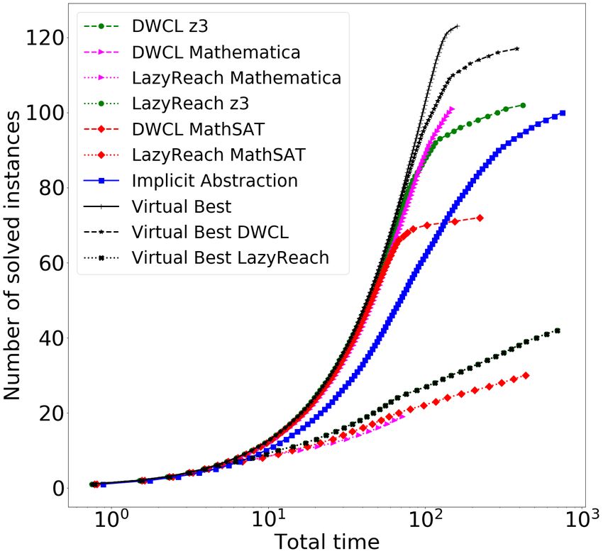
2         Authors Suppressed Due to Excessive Length

    To tackle the first problem, we consider the semi-algebraic decomposition
for dynamical systems of [34], also referred to as LZZ. The idea is to build
an abstraction from a given set of polynomials, partitioning the concrete state
space according to the sign of each polynomial. The abstraction is exact: there is
a transition from an abstract state to another abstract state if and only if there
is (at least) a concrete transition from the two concretizations of the abstract
states. Semi-algebraic decomposition is also appealing because it can be made
more precise adding new polynomials.
    The abstraction can be computed by means of logical operations (by repeat-
edly checking the satisfiability of quantifier-free formulas interpreted over the
reals). However, the second problem remains: the explicit computation of the
abstraction is extremely costly, since it requires the enumeration of all possi-
ble transitions between abstract states, that are exponential in the number of
considered polynomials.
    Interestingly, an effective use of abstraction is at the core of the most suc-
cessful verification techniques for discrete infinite-state transition systems. The
technique of predicate abstraction [17] was originally adapted for symbolic veri-
fication in [9] and then optimized in [20]. This idea has been further developed
in implicit predicate abstraction [37], that eliminates the burden of an upfront
exponential blowup in the computation of the abstract states by embedding the
abstraction in the symbolic encoding of the transitions. This approach has been
used also in combination with IC3 [6, 1, 7].
    In this paper, we propose a new approach to the verification of dynamical
systems with non-linear polynomial dynamics based on the use of semi-algebraic
decomposition. The contributions of the paper are the following:

    – We cast the problem of computing and verifying properties of dynamical sys-
      tems using the semi-algebraic decomposition in the framework of verification
      via implicit predicate abstraction (i.e., a first-order logic characterization of
      the semi-algebraic decomposition abstraction). Thus, we apply SMT-based
      model checking techniques to prove safety properties of polynomial dynam-
      ical systems.
    – We define a linear symbolic encoding for the abstraction. Note that the naive
      formulation of the predicate abstraction problem (which follows from the
      explicit computation approach propsed in [34]) is not effective in practice:
      in fact, the number of abstract states is exponential in the total number
      of polynomials that define the abstraction, and the encoding requires to
      enumerate all the possible pairs of abstract states to check the existence of
      an abstract transition. We exploit the properties of the LZZ formulation to
      define a coincise encoding that is linear in the number of the polynomials,
      hence making the approach feasible in practice.
    – We implement and experimentally evaluate the approach. The results show
      how the reduction to the verification of discrete infinite-state transition sys-
      tems is complementary to reachability analysis techniques and proves cases
      that were previously out of reach for the state-of-the-art tools.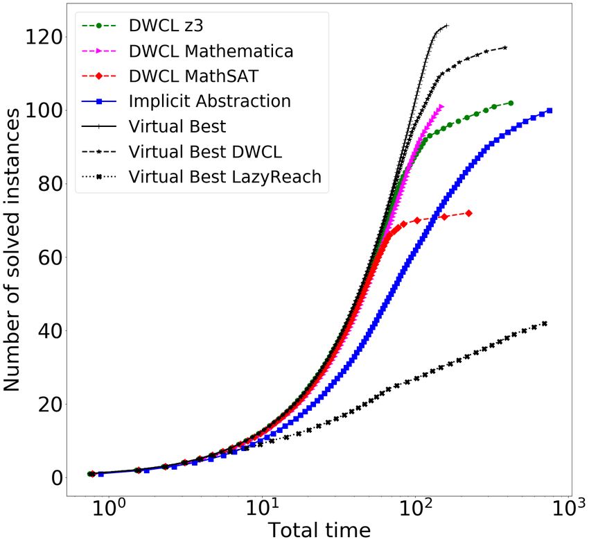
Implicit Semi-Algebraic Abstraction for Polynomial Dynamical Systems          3

Outline: The rest of the paper is structured as follows: Sec. 2 gives an overview
of the approach with a motivating example; Sec. 3 provides the background def-
initions; Sec. 4 shows the naive encoding of the abstraction, while in Sec. 5 we
derive the linear encoding and define the related implicit semi-algebraic abstrac-
tion; in Sec. 6, we present the experimental results; in Sec. 7, we discuss the
related work and, finally, in Sec. 8, we draw some conclusions and directions for
future work.

2   Overview of the approach

Consider a verification problem (adapted from [23]) on the non-linear dynamical
system with two variables x and y, and differential equations ẋ = −2y, ẏ = x2 .
We want to prove that the system cannot reach the set of bad states (x + 2)2 +
y 2 −1 ≤ 0 (i.e., it never leaves the safe region (x+2)2 +y 2 −1 < 0) when starting
from the initial set of states x − y − 21 ≥ 0 ∧ x + 2 > 0. Note that although in this
example the evolution of the system is not restricted, our approach can deal with
the more general case in which the evolution can be constrained by an invariant
condition that must always hold. The system is safe and will avoid the set of
bad states (see system’s dynamic in Figure 1).
    We can prove that the system is safe by first constructing and then model
checking a discrete semi-algebraic abstraction [34]: given the set of polynomials
A := {x − y − 21 , x + y + 21 , x + 2}, the semi-algebraic abstraction partitions
the state space according to the sign ({>,  0 ∧ x − y − 21 < 0 ∧ x + y + 12 < 0
represented as ○  1 in Figure 1b). There exists a transition from an abstract state
to another one if the two states are neighbors and there exists at least one tra-
jectory of the dynamical system going from one state to the other. The existence
of such condition can be checked using the LZZ algorithm [23], which checks if a
semi-algebraic set ψ is a differential invariant for a polynomial dynamical system
f˙ when its execution is restricted to the domain H (another semi-algebraic set).
The algorithm reduces the invariant check to the satisfiability of the Non-Linear
Real Arithmetic Theory formula LZZψ,f~,H (Z), where Z is a set of real-valued
variables. We can systematically check if there exists a transition from an ab-
stract state s1 to the abstract state s2 proving that s1 is not invariant when
restricted to the domain s1 ∨ s2 (i.e., checking that LZZs1 ,f~,s1 ∨s2 (Z) is false).
    Furthermore, we can use an algorithm, called LazyReach [34], to compute
the forward set of reachable abstract states starting from the initial states. As
usual, if no abstract states intersect the set of bad states then the system is
safe, and the reachable set of abstract states is a semi-algebraic invariant for
the system. Figure 1b shows the state space of the dynamical system: the initial
and bad states of the verification problem (represented with the green and red
region respectively), the solution of the polynomials from A (represented as
blue lines), and further superimpose the set of reachable abstract states and
transitions (represented as numbered circles and arrows between the circles).
4        Authors Suppressed Due to Excessive Length

                  (a)                                             (b)

Fig. 1. Safety verification problem and reachable states of the abstraction for the non-
linear dynamical system ẋ = −2y, ẏ = x2 , bad states (x + 2)2 + y 2 − 1 ≤ 0 (red
circle), and initial set of states x − y − 21 ≥ 0 ∧ x + 2 > 0 (green region). Figure (a)
shows the verification problem and the system’s vector field. Figure (b) shows the
reachable abstract states and the transitions of the algebraic abstraction (numbered
circles and arrows) computed using LazyReach and the differential invariant (green and
gray regions) obtained from the set of polynomials A = {x − y − 12 , x + y + 12 , x + 2}
(blue lines), computed using Implicit Abstraction. Abstract states represent different
combinations of signs for the abstraction’s polynomials. Examples of abstract states
are ○1 x+2 > 0∧x−y − 12 < 0∧x+y + 21 < 0, ○      2 x+2 > 0∧x−y − 21 = 0∧x+y + 21 < 0,
and ○ 3 x + 2 > 0 ∧ x − y − 12 = 0 ∧ x + y + 21 = 0.

The abstraction shown in Figure 1b is the result after applying LazyReach to
the verification problem.
     A main challenge for the LazyReach algorithm is to explicitly enumerate the
reachable states and transitions among them, since their number is exponential
in the number of polynomials A (i.e., the number of total states is already 3|A| ).
For the example above, where we have 3 polynomials, the maximum number of
states would be 27, with an even bigger number of transitions (e.g., one must
consider the transition between each pair of neighbouring abstract states). Even
if LazyReach enumerates the reachable abstract states on-the-fly, the explosion
in the number of states and transitions is still a bottleneck. Our implementation
of LazyReach applied to the above example explores a total of 9 states and checks
the existence of 27 transitions, taking about 12 seconds to complete.
     A possible solution to tackle the state explosion problem is the DWCL al-
gorithm, proposed in [34].The DWCL algorithm4 tries to reduce the number of
abstract states by checking if the sign of a polynomial a ∈ A is invariant, that
is if:
4
    We provide the main intuition behind the DWCL algorithm and we refer the reader
    to [34] for a detailed exposition.
Implicit Semi-Algebraic Abstraction for Polynomial Dynamical Systems             5

 – the sign of the polynomial a does not change in the initial states (i.e., the
   predicate a ./ 0, with ./∈ {, =}, holds for all the initial states); and
 – a ./ 0 is a continuous invariant for the dynamical system (this can be checked
   with LZZa./0,f~,H (Z).)

When a predicate a ./ 0 is a continuous invariant, the algorithm strengthens the
invariant of the dynamical system (by adding a ./ 0 to the invariants), allowing to
remove a from the set of polynomials A. While the DWCL algorithm may already
find a strong-enough invariant to prove the safety property, the algorithm falls
back to the LazyReach algorithm in the general case to explore the abstract
state space, hopefully with a strengthened invariant domain and a smaller set
of polynomials. In practice, the state-space explosion problem of LazyReach still
exists in the case “not enough” polynomials are sign-invariant, as it happens in
our motivating example. In the example, no polynomials are sign-invariant5 : this
means that the DWCL algorithm will not remove any polynomials from the set
A and LazyReach will still suffer from the state-space explosion problem.
    The semi-algebraic abstraction is a specific instance of predicate abstrac-
tion [17] of the dynamical system f~. For discrete-state systems, there exist effi-
cient algorithms to either explicitly compute the abstraction using Satisfiability
Modulo Theory (SMT) solvers [21, 20] or to implicitly represent the abstraction
and directly verify a safety property (e.g., implicit predicate abstraction [37]).
Since these algorithms work on a fully symbolic representation of the abstract
state space, they can cope with the state-space explosion due to the number of
predicates of the abstraction. However, applying the same symbolic-state tech-
niques to compute or verify the semi-algebraic abstraction is still challenging,
mainly because it requires to express the transition relation T (X, X 0 ) of the
semi-algebraic abstraction in a first-order logic formula. We can notice that such
transition relation T can be directly obtained from the abstraction’s definition6 :
                                                                      !
                      _
                                          0
             ∃Z.            s1 (X) ∧ s2 (X ) ∧ (¬LZZs1 ,f~,s1 ∨s2 (Z)) .
                     (s1 ,s2 )∈3A

The above transition relation enumerates all the possible pairs of abstract states
and its size is exponential in the number of polynomials in A. The additional
variables Z are copies of the state variables of the system and are used to encode
the LZZ condition. Clearly, even creating such formula is not scalable and hinders
the application of the standard abstraction and verification techniques used for
discrete systems.
    While the LZZ algorithm works for semi-algebraic sets (i.e., the candidate
invariant ψ and the invariant states H are both arbitrary Boolean combinations
5
    The differential-cut (DC) and the differential divide-and-conquer (DDC) proof rules
    used in DWCL fail for all the polynomials from A, so DWCL would not remove any
    polynomial.
6
    For clarity, here we do not include additional constraints in the transition relation,
    such as the neighborhood relation, which instead we consider later in Section 4.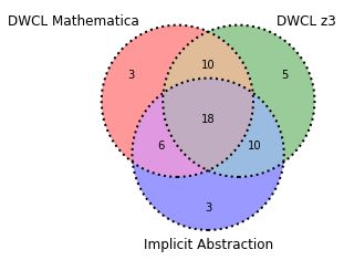
6       Authors Suppressed Due to Excessive Length

of non-linear arithmetic terms), here we apply LZZ to check the existence of a
transition between two abstract states.
    Our main contribution, presented in Section 5, is a compact formulation of the
above transition relation that has a size linear in the number of the polynomials
A. The steps to obtain such exponentially smaller transition are:
 1. We specialize the LZZ formula ¬LZZs1 ,f~,s1 ∨s2 (Z) to encode the existence of
    a transition between two abstract states s1 and s2 . The resulting formula is a
    disjunction, and each disjunct encodes the necessary and sufficient condition
    for a continuous transition to s2 to exist, either inside the set s1 (Z) or outside
    the set ¬s1 (Z). Intuitively, we obtain a specific encoding for checking the
    existence of an abstract transition, instead of reusing the LZZ as a “black
    box”.
 2. We “lift” the above disjunction to the disjunction of all the abstract states,
    obtaining the formula:

                  ∃Z.(InsExplf~(X, X 0 , Z) ∨ OutExplf~(X, X 0 , Z)),

    where InsExplf~(X, X 0 , Z) encodes the “inside condition” for all the pairs of
    transitions (and similarly for the “outside condition” OutExplf~(X, X 0 , Z)).
 3. The formula InsExplf~(X, X 0 , Z) still contains an explicit enumeration on
    the pair of abstract states. We show how we obtain an equivalent formula,
    InsSymbf~(X, X 0 , Z), that encodes the same condition for each polynomial
    a ∈ A in the abstraction, obtaining a linear, instead of exponential, encoding.
    We apply the same reasoning on OutExplf~(X, X 0 , Z).
    We then use the concise transition relation of T to obtain a symbolic tran-
sition system SbA that implicitly encodes the semi-algebraic abstraction for the
dynamical system f~ with the polynomials A. Technically, instead of computing
the predicate abstraction, we encode the implicit abstraction [37]. Consequently,
we avoid an expensive quantifier elimination step. We can then verify the safety
property on the transition system SbA using an SMT-based model checking al-
gorithm. We use the algorithm from [5], since SbA contains non-linear arithmetic
formulas. Our approach verifies the example of Figure 1 and finds the continuous
invariant:
           1                     1           1            1           1
(x − y <     ∨ x ≥ −2) ∧ (x − y ≥ ∨ x + y ≥ − ) ∧ (x − y ≥ ∨ x + y > − ),
           2                     2           2            2           2
which is shown in the union of the green and gray regions in Figure 1b.

3    Preliminaries
In this work, we consider first-order formulas in the theory of non-linear arith-
metic over the reals (NRA). We denote with φ(X) the formula φ containing free
variables from the set X = {x1 , . . . , xn }. We simplify the notation of the formula
φ(X) to φ when the set X is clear from the context.
Implicit Semi-Algebraic Abstraction for Polynomial Dynamical Systems 7
Invariant Verification for Polynomial Dynamical Systems
Safety Verification of Dynamical Systems. Given a set of variables X we write
X~ = [x1 , . . . , xn ]T to specify a vector containing all the variables in X ordered
lexicographically. We use the subscript X ~ i to access to the i-th element of the
vector. We focus on polynomial dynamical systems of ordinary differential equa-
tions (ODEs) Ẋ ~ = f~(X),
~ where Ẋ ~ is the vector of first-order derivatives of the
variables X ~ and f~(X) ~ is a vector of polynomials (i.e., f~i (X)
~ is a polynomial).
The safety verification problem consists of proving that every trajectory of the
dynamical system Ẋ ~ = f~(X)
~ starting inside the initial set of states ψ and while
being inside the evolution domain constraints H remains inside the safe set of
states φ. We can write the problem using differential dynamic logic [29] notation:
~ = f~(X)
ψ → [Ẋ ~ & H]φ. (1)
The solution to the intial value problem ~x0 ∈ Rn is a differentiable function
ϕ(~x0 , t) : Rn+1 → Rn such that dt
d
(ϕ(~x0 , t)) = f~(ϕ(~x0 , t)). The system is safe if
the following holds:
∀~x0 ∈ ψ.∀τ ≥ 0.(∀t ∈ [0, τ ].ϕ(~x0 , t) ∈ H) → ϕ(~x0 , t) ∈ φ).
Proving the system is safe amounts to find a formula θ(X) such that: i) H ∧ ψ →
~ = f~(X)
θ, ii) θ → [Ẋ ~ & H] θ, and iii) θ → φ. Essentially θ(X) is a continuous
invariant [30] that contains the initial states and that is contained in the safe
states.
LZZ Algorithm [23]. The LZZ algorithm reduces the problem of checking if θ is
a continuous invariant to checking the validity of the following formula:
˙ ((θ(X) ∧ H(X) ∧ Inf~,H (X)) → Inf~,θ (X))∧
LZZθ,f~,H (X) = (2)
((¬θ(X) ∧ H(X) ∧ In−f~,H (X)) → ¬In−f~,θ (X)),
where the formula Inf~,γ (X) for the ODEs f~ and the formula γ represents the set
of states which will evolve inside the set γ for some non-zero time in the future.
Respectively, the formula In−f~,γ (X) represents the set of states evolved inside
the set γ for some non-zero time in the past, and −f~ represents the dynamical
system evolving in “reverse”. Note that the construction of the formula Inf~,γ (X)
assumes γ to be in disjunctive normal form (DNF):
_ ^
γ= a(X) ./ 0,
d∈disj(γ) a./0∈pred(d)
where disj(γ) enumerates the disjuncts of a formula γ, pred(d) enumerates the
predicates in the disjunct d, and ./∈ {>, ≥}7 . The formula Inf~,γ (X) is defined
7
Later we also consider predicates p = 0. The construction of Inf~,a=0 (X) can be
found in [12].8 Authors Suppressed Due to Excessive Length
as:
_ ^
Inf~,γ (X) = Inf~,a./0 (X). (3)
d∈disj(γ) a./0∈pred(d)
The formula Inf~,a./0 (X) encodes the set for a single predicate a ./ 0 using the Lie
derivatives of the polynomial a(X). The i-th Lie derivative Lif~a of a polynomial
a(X) with respect to the ODEs f~ is defined recursively as:
(0) (i) ∂ (i−1) ~
L~ a =
˙ a, L~ a =
˙ L af .
f f
∂X~ f~
Inf~,a>0 (X) encodes that the first non-zero Lie derivative of a must be positive
in order for the trajectories of the system to enter the set a > 0 and stay inside
the set for a positive time8 (see [23] and [12] for a thorough explanation):
!
_ ^ (j) (i)
Inf~,a>0 (X) =
˙ L~ a = 0 ∧ L~ a > 0 , (4)
f f
0≤i≤Na,f 0≤j0 (X) ∨
Inf~,a≥0 (X) = L ~ a = 0, (5)
f
0≤i≤Na,f
where Na,f~ is an integer constant and is an upper bound on the minimum integer
(r)
number r (called rank ) such that L ~ a 6= 0 (for all x ∈ Rn ). Na,f~ can be
f
computed using Gröbner basis as explained in [23].
In the following, we will only use the fact that the formula Inf~,γ (X) for the
DNF formula γ is the DNF formula where Inf is applied to the predicates (as
shown in Formula (3)).
Semi-Algebraic Abstraction [34]. The semi-algebraic abstraction of the dynami-
~ = f~(X)
cal system Ẋ ~ partitions its state space with respect to a set of polyno-
mials A =˙ {a1 , . . . , am }. The abstraction is the (explicit state) transition system
˙ h3A , If,A , Tf,A i where:
SA =
˙ {s = a∈A a ./ 0 |./∈ {>, 0)
to a state where the same predicate is less than 0 (e.g., a < 0), and
vice-versa. The abstraction does not visit two abstract states containing
predicates with opposite signs, forcing instead to visit the intermediate
state where the predicate is equal to 0.
8
In our implementation we encode Inf~,a>0 (X) using the remainders of the Lie deriva-
tive, as in [12].Implicit Semi-Algebraic Abstraction for Polynomial Dynamical Systems 9
• There exists a continuous trajectory from s1 to s2 . This condition corre-
sponds to checking that the following differential dynamic logic formula
is not valid (i.e. s1 is not a differential invariant when restricting the
evolution domain to s1 ∨ s2 ):
~ = f~(X)
s1 → [Ẋ ~ & s1 ∨ s2 ]s1 ,
which can be checked using the sound and complete LZZ algorithm, i.e.
checking the satisfiability of the first-order formula ¬LZZs1 ,f~,s1 ∨s2 (Z)).
Since the number of states 3A is finite we can compute the set of reachable states.
The concretization of this set, θ contains the initial states and is a differential
invariant. If θ further implies the safe states ψ, then we prove the safety verifi-
cation problem 1. However, the computation of the abstract transition relation
is exponential in the number of polynomials in A because we would need to
enumerate all the possible pairs of transitions (s1 , s2 ) ∈ 3A × 3A .
Predicate Abstraction.
A symbolic transition system S is a tuple S =hV, ˙ I, T i, where V is a set of (state)
variables, I(V ) is a formula representing the initial states, and T (V, V 0 ) is a
formula representing the transition relation. A state s of S is an interpretation
of the state variables V . A (finite) path π of S is a finite sequence π =s ˙ 0 , s1 , . . . , sk
of states with the same domain and interpretation of symbols in the signature
Σ: such that s0 |= I and for all i, 0 ≤ i < k, si , s0i+1 |= T . We say that a state s is
reachable in S iff there exists a path of S ending in s. Given a formula P (V ) and
a transition system S, the invariant verification problem, denoted with S |= P ,
checks if for all the finite paths s0 , s1 , . . . , sk of S, for all i, 0 ≤ i ≤ k, si |= P .
Predicate Abstraction [17] partitions the concrete system S = hV, I, T i ac-
cording to a finite set of predicates P ={p˙ 1 , . . . , pk } in a finite symbolic transition
system:
SbP = hVP , IbP (VP ), TbP (VP , VP0 )i
using a new abstract Boolean variable vp for each predicate p (VP = {vV p |v ∈V}
is the set of those new variables). The abstraction relation HP (V, VP ) =
˙ p∈P vp ↔
p(V ) defines how a set of concrete states is abstracted to the abstract states.
We compute the abstraction of a formula ψ(V ) by existentially quantifying the
concrete variables V :
˙ ∃V.(ψ(V ) ∧ HP (V, VP )).
ψbP (VP ) =
Similarly, we compute the abstract transition relation for T (V, V 0 ):
TbP (VP , VP0 ) =
˙ ∃V, V 0 .(T (V, V 0 ) ∧ HP (V, VP ) ∧ HP (V 0 , VP0 )).
The above formulation is sufficient to compute the predicate abstraction for an
infinite-state transition system S = hV, I, T i and a set of predicates P. However,
the main challenge in computing the abstraction is to eliminate the quantifiers,
since quantifier elimination is expensive to compute.10 Authors Suppressed Due to Excessive Length
Implicit Predicate Abstraction. Implicit Predicate Abstraction [37] is a model
checking algorithm that avoids computing the abstract version of the initial
states, safety property, and transition relation, insteads it encodes the existence
of a path in the abstract system. It exploits the fact that the abstraction induces
an equivalence relation among concrete states of the system (i.e., two concrete
states are equivalent if they belong to the same abstract state) and that this
relation can be expressed as a quantifier free formula:
^
EQP (V, V ) =
˙ p(V ) ↔ p(V ). (6)
p∈P
We use the equivalence EQP (V, V ) to relate two sets of concrete states and
we encode the problem of reaching a set of target states ¬P in k steps of the
transition system S as follows:
0
BM CPk =
˙ I(V 0 ) ∧ EQP (V 0 , V ) ∧
^ h−1 h
k−1
T (V , V h ) ∧ EQP (V h , V ) ∧ T (V , V k) ∧
1≤h, <
, =}}, and the set of abstract variables VP is defined as in Section 3 (i.e., the ab-
straction contains a Boolean variable vp for each predicates p ∈ P). We similarly
use the formula HP (X, VP ) to describe the equivalence relation of the concrete
states. The formulas IbP (VP ) and ¬P
dP (VP ) are the semi-algebraic abstraction of
the initial states ψ and of the unsafe states ¬φ:
˙ ∃X.(ψ(X) ∧ HP (X, VP )),
IbP (VP ) = ¬P ˙ ∃X.(¬φ(X) ∧ HP (X, VP )),
dP (VP ) =Implicit Semi-Algebraic Abstraction for Polynomial Dynamical Systems 11
and we obtain the abstraction by existentially quantifying the concrete variables
X. The definition of the abstract transition relation TbP (VP , VP0 ), which differs
from the encoding of the semi-algebraic decomposition, is:
TbP (VP , VP0 ) =
˙ ∃X, X 0 . N(X, X 0 ) ∧ H(X) ∧ H(X 0 )∧ (7)
!
0
HP (X, VP ) ∧ HP (X , VP0 ) 0
∧ ∃Z.TA (X, X , Z) ,
where N(X, X 0 ) encodes the adjacent relation between abstract states:
^
N(X, X 0 ) = (a(X) < 0 → a(X 0 ) ≤ 0) ∧ (a(X) > 0 → a(X 0 ) ≥ 0) ,
a∈A
and TA (X, X 0 , Z) encodes the existence of a transition in the dynamical system
f~ for each pair of abstract states (s1 , s2 ) ∈ 3A :
_
TA (X, X 0 , Z) =
˙ s1 (X) ∧ s2 (X 0 ) ∧ ¬LZZs1 ,f~,s1 ∨s2 (Z) . (8)
(s1 ,s2 )∈3A
Theorem 1. The transition systems SA and SbA are bisimilar.
Corollary 1. SA |= ¬¬P ~ = f~(X)
dP (VP ) implies ψ → [Ẋ ~ & H]φ.
Proof (sketch). The proof follow directly from Theorem 1. t
u
While the encoding of the transition relation TbP (VP , VP0 ) is symbolic, it (and in
particular the sub-formula TA (X, X 0 , Z)) explicitly enumerates an exponential
number of abstract pair of states. Clearly, this encoding is not practical and
defeats the purpose of using symbolic techniques to compute the abstraction.
5 Linear Encoding of the Semi-Algebraic Abstraction
Specializing the LZZ formula for checking abstract transitions
The construction of the semi-algebraic abstraction uses the formula ¬LZZs1 ,f~,s1 ∨s2 (Z)
to encode the existence of a transition from the abstract state s1 to the abstract
state s2 . We observe that here the LZZ algorithm is applied to formulas with a
specific structure – the abstract states s1 (Z) and s2 (Z), in contrast to arbitrary
semi-algebraic sets as in the general case of LZZθ,f~,H (X) where the formulas θ
and H are in DNF. Instead, in the case of LZZs1 ,f~,s1 ∨s2 (Z), each abstract state
si (X) assigns a sign to each polynomial a ∈ A and is represented as conjunctions
of predicates si = a1 ./1 0 ∧ a2 ./2 0 ∧ . . . am ./m 0, where
V ./j ∈ {>,12 Authors Suppressed Due to Excessive Length
note that the evolution domain constraints are also a disjunction of two abstract
states s1 ∨ s2 .
We specialize the Eq. (2) to the specific case of LZZs1 ,f~,s1 ∨s2 (Z). We will
use such specialization to obtain a compact (linear in the number of polynomi-
als) encoding later in the section. Instantiating the formula (2) to the case of
LZZs1 ,f~,s1 ∨s2 (Z), we get:
LZZs1 ,f~,s1 ∨s2 (Z) =
˙
((s1 (Z) ∧ (s1 (Z) ∨ s2 (Z)) ∧ Inf~,s1 ∨s2 (Z)) → Inf~,s1 (Z))∧ (9)
((¬s1 (Z) ∧ (s1 (Z) ∨ s2 (Z)) ∧ In−f~,s1 ∨s2 (Z)) → ¬In−f~,s1 (Z))
Applying the Boolean identities: (α ∧ (α ∨ β)) ↔ α, (¬α ∧ (α ∨ β)) ↔ ¬α ∧ β
⇐⇒((s1 (Z) ∧ Inf~,s1 ∨s2 (Z)) → Inf~,s1 (Z))∧ (10)
((¬s1 (Z) ∧ s2 (Z) ∧ In−f~,s1 ∨s2 (Z)) → ¬In−f~,s1 (Z))
Rewriting the implication and applying De Morgan’s laws:
⇐⇒(¬s1 (Z) ∨ ¬Inf~,s1 ∨s2 (Z) ∨ Inf~,s1 (Z))∧ (11)
(s1 (Z) ∨ ¬s2 (Z) ∨ ¬In−f~,s1 ∨s2 (Z) ∨ ¬In−f~,s1 (Z))
Expanding the definition of In (Eq. (3)): Inf~,α∨β =
˙ (In−f~,α ∨ Inf~,β )
˙ (In−f~,α ∨ In−f~,β )
In−f~,α∨β =
⇐⇒(¬s1 (Z) ∨ ¬(Inf~,s1 (Z) ∨ Inf~,s2 (Z)) ∨ Inf~,s1 (Z))∧ (12)
(s1 (Z) ∨ ¬s2 (Z) ∨ ¬(In−f~,s1 (Z) ∨ In−f~,s2 (Z)) ∨ ¬In−f~,s1 (Z))
Applying the Boolean identities: (¬(α ∨ β) ∨ α) ↔ (¬β ∨ α), (¬(α ∨ β) ∨ ¬α) ↔ ¬α
⇐⇒(¬s1 (Z) ∨ ¬Inf~,s2 (Z) ∨ Inf~,s1 (Z))∧ (13)
(s1 (Z) ∨ ¬s2 (Z) ∨ ¬In−f~,s1 (Z)).
Note that when we expand the definition of Inf~,s1 ∨s2 (Eq. (12)), the formula
s1 ∨ s2 is in DNF and that In does not distribute over arbitrary Boolean for-
mulas (see [12]). Thus, Formula (13) is equivalent to the initial Formula (9) of
LZZs1 ,f~,s1 ∨s2 (Z). We then write the negation of the Formula 13 as:
¬LZZs1 ,f~,s1 ∨s2 (Z) =
˙ (s1 (Z) ∧ Inf~,s2 (Z) ∧ ¬Inf~,s1 (Z))∨ (14)
(¬s1 (Z) ∧ s2 (Z) ∧ In−f~,s1 (Z)).
Linear Encoding of the Semi-Algebraic Transition Relation
In the following steps, we revise the formula TA (X, X 0 , Z) that encodes the ex-
istence of the transitions in the abstraction, still enumerating all possible pairs
of states, using the specialized LZZ encoding from Eq. (14). We substitute the
subformula ¬LZZs1 ,f~,s1 ∨s2 (Z) with the specialized LZZ encoding (Eq. (16)); we
then distribute the conjunction s1 (X)∧s2 (X 0 ) over the disjunction present in theImplicit Semi-Algebraic Abstraction for Polynomial Dynamical Systems 13
definition of ¬LZZs1 ,f~,s1 ∨s2 (Z) (Eq. (17)), and then over possible pairs of states
(Eq. (18)). We rename the two disjuncts in Eq. (18) as InsExplf~(X, X 0 , Z)
and OutExplf~(X, X 0 , Z)) (Eq. (19)). The formulas InsExplf~(X, X 0 , Z) and
OutExplf~(X, X 0 , Z)) still enumerate explicitly the abstract states. However,
each of these formulas is a conjunction of predicates, application of the Inf~
operator to a conjunction of predicates, and negations of the application of Inf~.
TA (X, X 0 , Z) =
˙
_
∃Z. (s1 (X) ∧ s2 (X 0 ) ∧ ¬LZZs1 ,f~,s1 ∨s2 (Z)) (15)
(s1 ,s2 )∈3A
!
_ s1 (X)∧s2 (X 0 )∧((s1 (Z)∧Inf~,s (Z)∧¬Inf~,s (Z))∨
⇐⇒∃Z. 2 1
(¬s1 (Z)∧s2 (Z)∧In−f~,s (Z)))
(16)
1
(s1 ,s2 )∈3A
!
_ (s1 (X)∧s2 (X 0 )∧s1 (Z)∧Inf~,s (Z)∧¬Inf~,s (Z))∨
⇐⇒∃Z. 2
((s1 (X)∧s2 (X 0 )∧¬s1 (Z)∧s2 (Z)∧In−f~,s (Z))
1
(17)
1
(s1 ,s2 )∈3A
!
(s1 (X)∧s2 (X 0 )∧s1 ∧Inf~,s (Z)∧¬Inf~,s (Z))∨
W
⇐⇒∃Z. (s1 ,s2 )∈3A
W 2
(s1 (X)∧s2 (X 0 )∧¬s1 ∧s2 ∧In−f~,s (Z))
1
(18)
(s1 ,s2 )∈3A 1
⇐⇒∃Z.(InsExplf~(X, X 0 , Z) ∨ OutExplf~(X, X 0 , Z)). (19)
We now show how we obtain a formula InsExplf~(X, X 0 , Z) with a linear
size. We expand the definition of the formula InsExplf~(X, X 0 , Z) with respect
to the predicates in s1 and s2 . Recall that each abstract state is aVconjunction
of predicates obtained from the set of polynomial A (i.e., s = ˙ a∈A a ./a 0,
./a ∈ {>,14 Authors Suppressed Due to Excessive Length
the abstract states s1 and s2 , instead of the pairs of abstract states:
^
InsSymbf~(X, X 0 , Z) =˙ a(X) ./ 0 → a(Z) ./ 0 ∧ (21)
a∈A,./∈{>,,, 0, a < 0, and a = 0 are mutually exclusive). We show that µ is an in-
terpretation for all the conjuncts in InsSymbf~(X, X 0 , Z). We have that µ |=
a∈A,./∈{>,,,Implicit Semi-Algebraic Abstraction for Polynomial Dynamical Systems 15
Hence, µ is a model for at least one of the disjuncts in InsExplf~(X, X 0 , Z). t
u
We provide a detailed proof of the lemma in the Appendix A. We similarly define
the compact encoding of OutExplf~(X, X 0 , Z):
^
OutSymbf~(X, X 0 , Z) =
˙ a(X) ./ 0 → In−f~,a./0 (Z) ∧ (22)
a∈A,./∈{>,,,16 Authors Suppressed Due to Excessive Length
where
TImpl,P (X, X 0 , Z) =
˙ N(X, X 0 ) ∧ H(X) ∧ H(X 0 )∧ (24)
0 0
(InsSymbf~(X, X , Z) ∨ OutSymbf~(X, X , Z)).
We can prove that SImpl,P |= P (X) iff SbP |= ¬¬P
dP (VP ). This way, we can
model check the transition system SImpl,P |= P to prove a property on the
dynamical system.
Theorem 3. SImpl,P |= P (X) iff SbP |= ¬¬P
dP (VP ).
6 Experimental Evaluation
Research Questions
We evaluate the performance of our approach (Implicit Abstraction) for the
verification of invariant properties on the semi-algebraic abstraction of dynamical
systems. Implicit Abstraction first encodes the semi-algebraic abstraction in a
transition system (as we show in Section 5), and then model checks the invariant
on the transition system with an off-the-shelf model checker. Our experiments
aim to answer the following research questions:
RQ 1: How does Implicit Abstraction compare with the LazyReach algorithm [34],
which explicitly enumerates the reachable states of the abstraction?
RQ 2: How does Implicit Abstraction compare with the DWCL algorithm [34],
which applies a divide-and-conquer strategy to reduces the number of polyno-
mials in the abstraction?
Experimental Setup
We implemented the construction of the implicit abstraction transition system
in Python using PySMT [11] to manipulate formulas, and SymPy [24] for poly-
nomial manipulation and Gröbner bases computation (i.e., to compute the Lie
derivatives’ ranks). We verify the implicit abstraction transition system with
the model checking algorithm for symbolic transition systems with NRA con-
straints from [5], which uses the MathSAT [8] SMT solver and incrementally
over-approximates the non-linear arithmetic formulas with formulas in the theo-
ries of linear arithmetic and uninterpreted functions. We implemented both the
LazyReach and the DWCL algorithms in the same Python tool. Our implemen-
tation of DWCL can use different backends to decide the satisfiability of NRA
formulas, namely MathSAT , the z3 SMT solver [26], or Mathematica [18].
We consider 90 invariant verification problems for dynamical systems from
the KeyMaera X theorem prover [10]. These problems are a superset of the
ones used in [34] and are used in the Applied Verification of Continuous and
Hybrid Systems (ARCH) competition [25]. We obtain a total of 180 benchmark
instances using, for each problem, two sets of polynomials for the semi-algebraicImplicit Semi-Algebraic Abstraction for Polynomial Dynamical Systems 17
abstraction. The first set contains all the factors of the righ-hand side of the
ODEs; the second one extends the first by including also the Lie derivatives of
the polynomials. The latter set induces an abstraction that is more precise but
also has a larger state-space.
We evaluate the performance of the algorithms Implicit Abstraction, LazyReach,
and DWCL to solve the above verification problems. The underlying problem re-
quires to decide the satisfiability of NRA formulas, and the decision procedures
for this problem are efficient for different subset of problems. For this reason
we further evaluate different configurations of the LazyReach and DWCL al-
gorithms using three different solvers for NRA formulas (MathSAT , z3 , and
Mathematica). We remark that using a different SMT solver in the model check-
ing algorithm, which we use in Implicit Abstraction, is more difficult because the
solver is tightly integrated in the tool implementation.
We run the Implicit Abstraction, LazyReach, and DWCL algorithm on all the
180 benchmark instances with a time out of 100 seconds, and we measure the
execution times to either prove (safe result) or find an abstract counterexam-
ple (unknown result) for each instance. An archive containing the necessary to
reproduce the experiments is available online at omitted for double blind review.
Results
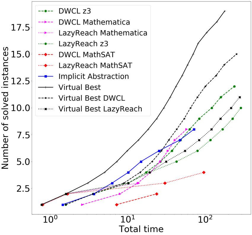
RQ 1 - Implicit Abstraction vs. LazyReach. From the cumulative plot in Fig-
ure 2, we see that Implicit Abstraction almost always outperforms LazyReach.
From the cumulative plot in Figure 2a we see that Implicit Abstraction signif-
icantly outperforms LazyReach on safe instances. For better readability, in the
plot we only show the (virtual) portfolio algorithm running each configuration
of LazyReach, Virtual Best LazyReach, obtaining by considering the best run
time among the different configurations of LazyReach using different backend
solvers. Virtual Best LazyReach solves a total of 42 safe instances, while Implicit
Abstraction solves 100 safe instances. The scatter plots shown in the first row of
Figure 3 confirms the same intuition (note that the safe instances represented
as blue circles are mostly in the lower-right triangle of the plot).
Figure 2b shows the cumulative plot when verifying unknown instances. Note
that the total number of unknown instances in the benchmarks are much smaller
than the safe ones (combining the results of all the algorithms we have 123
safe instances, 19 unknown instances, and 38 still unsolved instances). From
Figure 2b, we see that the performance of Implicit Abstraction is comparable
with LazyReach, solving a total of 8 instances and 11 instances respectively.
RQ 2 - Implicit Abstraction vs. DWCL. From the cumulative plots in Figure 2,
the Virtual Best DWCL solves 37 more instances than Implicit Abstraction. How-
ever, we also see from Figure 2 that the global Virtual Best solves more instances
and is faster than Virtual Best DWCL. In fact, Implicit Abstraction is orthogonal
to DWCL and is comparable to DWCL when fixing either Mathematica or z3
(Implicit Abstraction solves 108 instances, DWCL Mathematica solves 109, and
DWCL z3 solves 114).18 Authors Suppressed Due to Excessive Length
The scatter plots in the second row of Figure 3 compare Implicit Abstraction
with DWCL MathSAT , DWCL Mathematica, and DWCL z3 . From these plots,
we see that there are several instances that are solved by only one of the two
algorithms compared in each plot. While we see similar data when comparing
Implicit Abstraction with Virtual Best DWCL (always in the scatter plots of Fig-
ure 3), the number of instances solved uniquely by Implicit Abstraction seems
smaller. We get a more precise picture of the complementarity of Implicit Ab-
straction, DWCL Mathematica, and DWCL z3 from the diagrams in Figure 4,
where we can clearly see that Implicit Abstraction is orthogonal to both DWCL
Mathematica and DWCL z3 . From the diagram, we see that when using a differ-
ent backend (i.e., Mathematica or z3 ) DWCL solves a different set of instances.
This difference in performance using Mathematica and z3 is not surprising since
Mathematica and z3 uses different algorithms to solve formulas in NRA.
We further notice that Implicit Abstraction uses the MathSAT SMT solver
in the backend, and from our experiments (see again Figure 3) DWCL MathSAT
performs quite poorly compared to both DWCL Mathematica and DWCL z3 .
While naively replacing MathSAT in the model checking algorthm we use [5]
would not provide a significant performance improvement, it is reasonable to
think that investigating a tighter integration with either z3 or Mathematica could
improve the model checking performance. However, we believe this integration
to be beyond the scope for this paper, where we enable the use of symbolic model
checking techniques to analyze the semi-algebraic decomposition.
(a) Safe instances (b) Unknown instances
Fig. 2. Plots the total number of instances (on the y axis) in function of the cumulative
time (in seconds, on the x axis) took by Implicit Abstraction, LazyReach, and DWCL
to solve (a) safe and (b) unknown instances. The comparison includes the results of
LazyReach and DWCL using different (MathSAT , z3 , and Mathematica), as well as
virtual portfolios combining the best results obtained by a given algorithm when run
with multiple backends. We omit some configurations in (b) to improve readability.Implicit Semi-Algebraic Abstraction for Polynomial Dynamical Systems 19
Fig. 3. Scatter plots comparing the run time (in seconds) of Implicit Abstraction (on
the y axis) with LazyReach (first row, on the x axis) and DWCL (second row, on the x
axis). Blue circles represent safe verification problems. Red crosses are instances where
the algorithm found an abstract counterexample. When Implicit Abstraction runs for
more than the 100 seconds time out, we plot the instance on the vertical line marked
as to, and similarly for LazyReach and DWCL on the horizontal line.
7 Related work
In this work, we focus on the (unbounded time) safety verification problem for
polynomial dynamical systems. Such problem is relevant when proving safety for
hybrid programs [28] with Keymaera X [10] or for hybrid CPS with the HHL
Prover [38]. Our reduction to transition systems may be used as sub-procedure
in both theorem provers to automate the search of a continuous invariant.
There exist different techniques to prove safety properties for polynomial
dynamical systems (see e.g., [13]): barrier certificates [31, 19], first integrals [15],
and Darboux Polynomials [16]. All these techniques are orthogonal to semi-
algebraic abstraction, and can be used to find invariant polynomials to restrict
the abstract state space. Pegasus [35] implements all the above techniques, the
LazyReach, and DWCL algorithms. Our algorithm can be integrated in Pegasus.
The LZZ [23] procedure has been originally proposed to synthesize a continuous
invariant. Instead, we use the LZZ procedure to encode the abstract transition
relation, and then we prove a safety property in the abstraction. We also provide
a specialized encoding of LZZ to check the existence of abstract transitions.
The semi-algebraic abstraction [34] is a qualitative abstraction [36, 39]. In
this work, we propose a different algorithm to verify semi-algebraic abstractions
that allows us to explore the abstract state-space symbolically, in contrast to
the LazyReach algorithm [34]. In principle, our technique is orthogonal to the
DWCL algorithm [34], since we could replace LazyReach, which is used in DWCL
as a sub-routine, with our approach (i.e., model check the implicit abstraction).20 Authors Suppressed Due to Excessive Length
(a) All the instances (b) Safe instances (c) Unknown instances
Fig. 4. Diagrams representing the distribution of unique instances solved combining
different algorithms (DWCL Mathematica, DWCL z3 , and Implicit Abstraction). Each
set, displayed as a dotted circle enclosed by a dotted line, represents the set of instances
solved with one algorithm. The number shown in each partition is the number of
instances solved uniquely by the sets forming the partition. For example, the central
partition (i.e, the intersection of all the sets) of the diagram (a) shows that DWCL
Mathematica, DWCL z3 , and Implicit Abstraction solved the same set of 141 instances.
Relational abstraction [33] abstracts the dynamical system’s trajectories with
a discrete transition relation, reducing the verification problem on the continuous
system to a verification problem on the discrete system. The implicit encoding
of the semi-algebraic abstraction can be seen as an instance of relational ab-
straction, where a trajectory of the dynamical system is mapped to a sequence
of abstract transitions (similarly to what happen with relational abstractions for
time-sampled systems in [40, 3]). Since relational abstractions can be composed
with each other (e.g., see [27]), we can strengthen the implicit semi-algebraic
abstraction encoding with a relational abstraction. This composition is useful
in the case the semi-algebraic abstraction cannot easily capture the system’s
behavior (e.g., a precise relation of the time elapsed in a transition [27]).
Predicate abstraction [17] is a commonly used abstraction techniques to verify
infinite-state systems. Several symbolic techniques [20, 21, 4] focus on the efficient
computation of the predicate abstraction. In principle, we can also use those
technique to explicitly compute the semi-algebraic abstraction. However, the
up-front, explicit computation of the abstraction is a bottleneck and can be
avoided with implicit predicate abstraction [37] when the goal is to verify a
safety property on the abstract system. We use implicit abstraction to obtain
an implicit encoding of the semi-algebraic abstraction. The transition system of
the semi-algebraic abstraction contains NRA formulas (the polynomials can be
non-linear or the Lie derivative of the polynomials are non-linear). While there
are few algorithms and tool that can verify such transition systems (e.g., [5]),
our technique is agnostic to the underlying model checking algorithm.
8 Conclusions and Future Work
In this paper, we addressed the safety problem of polynomial dynamical systems.
We built on the LZZ algorithm to define a symbolic encoding of the abstractionImplicit Semi-Algebraic Abstraction for Polynomial Dynamical Systems 21
based on a set of polynomials. The encoding is linear in the number of polynomi-
als and can be used to implicitly represent the abstraction without the need of
enumerating the abstract states, enabling the use of SMT-based model checking
techniques. The experimenal evaluation showed that the approach is promising
and complementary to existing techniques solving a number of new instances.
The main directions for future works are, on one side, refining the abstraction
discovering new polynomials that are able to remove spurious abstract counterex-
amples, and, on the other side, the application of the approach to hybrid systems
where the continuous dynamics depends on the discrete state of the system.
Acknowledgements S. Mover was partially supported by ... A. Cimatti, A.
Griggio, and S. Tonetta were partially supported by ECSEL JU under grant
agreement No 876852. The JU receives support from EU’s H2020 programme,
Austria, Czech Republic, Germany, Ireland, Italy, Portugal, Spain, Sweden, Turkey.22 Authors Suppressed Due to Excessive Length References 1. Birgmeier, J., Bradley, A.R., Weissenbacher, G.: Counterexample to induction- guided abstraction-refinement (CTIGAR). In: Biere, A., Bloem, R. (eds.) Com- puter Aided Verification - 26th International Conference, CAV 2014, Held as Part of the Vienna Summer of Logic, VSL 2014, Vienna, Austria, July 18- 22, 2014. Proceedings. Lecture Notes in Computer Science, vol. 8559, pp. 831– 848. Springer (2014). https://doi.org/10.1007/978-3-319-08867-9_55, https:// doi.org/10.1007/978-3-319-08867-9\_55 2. Chakraborty, S., Jerraya, A., Baruah, S.K., Fischmeister, S. (eds.): Proceedings of the 11th International Conference on Embedded Software, EMSOFT 2011, part of the Seventh Embedded Systems Week, ESWeek 2011, Taipei, Taiwan, October 9-14, 2011. ACM (2011) 3. Chen, X., Mover, S., Sankaranarayanan, S.: Compositional relational abstrac- tion for nonlinear hybrid systems. ACM Trans. Embedded Comput. Syst. 16(5), 187:1–187:19 (2017). https://doi.org/10.1145/3126522, https://doi.org/ 10.1145/3126522 4. Cimatti, A., Franzén, A., Griggio, A., Kalyanasundaram, K., Roveri, M.: Tighter integration of bdds and smt for predicate abstraction. In: 2010 Design, Automation & Test in Europe Conference & Exhibition (DATE 2010). pp. 1707–1712. IEEE (2010) 5. Cimatti, A., Griggio, A., Irfan, A., Roveri, M., Sebastiani, R.: Incremental lin- earization for satisfiability and verification modulo nonlinear arithmetic and transcendental functions. ACM Trans. Comput. Log. 19(3), 19:1–19:52 (2018). https://doi.org/10.1145/3230639, https://doi.org/10.1145/3230639 6. Cimatti, A., Griggio, A., Mover, S., Tonetta, S.: IC3 modulo theories via im- plicit predicate abstraction. In: Ábrahám, E., Havelund, K. (eds.) Tools and Algorithms for the Construction and Analysis of Systems - 20th International Conference, TACAS 2014, Held as Part of the European Joint Conferences on Theory and Practice of Software, ETAPS 2014, Grenoble, France, April 5- 13, 2014. Proceedings. Lecture Notes in Computer Science, vol. 8413, pp. 46– 61. Springer (2014). https://doi.org/10.1007/978-3-642-54862-8_4, https://doi. org/10.1007/978-3-642-54862-8\_4 7. Cimatti, A., Griggio, A., Mover, S., Tonetta, S.: Infinite-state invariant check- ing with IC3 and predicate abstraction. Formal Methods in System Design 49(3), 190–218 (2016). https://doi.org/10.1007/s10703-016-0257-4, https://doi. org/10.1007/s10703-016-0257-4 8. Cimatti, A., Griggio, A., Schaafsma, B.J., Sebastiani, R.: The mathsat5 SMT solver. In: Piterman, N., Smolka, S.A. (eds.) Tools and Algorithms for the Construction and Analysis of Systems - 19th International Confer- ence, TACAS 2013, Held as Part of the European Joint Conferences on Theory and Practice of Software, ETAPS 2013, Rome, Italy, March 16-24, 2013. Proceedings. Lecture Notes in Computer Science, vol. 7795, pp. 93– 107. Springer (2013). https://doi.org/10.1007/978-3-642-36742-7_7, https:// doi.org/10.1007/978-3-642-36742-7\_7 9. Flanagan, C., Qadeer, S.: Predicate abstraction for software verification. In: Launchbury, J., Mitchell, J.C. (eds.) Conference Record of POPL 2002: The 29th SIGPLAN-SIGACT Symposium on Principles of Program- ming Languages, Portland, OR, USA, January 16-18, 2002. pp. 191–202. ACM (2002). https://doi.org/10.1145/503272.503291, https://doi.org/10.1145/ 503272.503291
Implicit Semi-Algebraic Abstraction for Polynomial Dynamical Systems            23

10. Fulton, N., Mitsch, S., Quesel, J., Völp, M., Platzer, A.: Keymaera X: an
    axiomatic tactical theorem prover for hybrid systems. In: Felty, A.P., Mid-
    deldorp, A. (eds.) Automated Deduction - CADE-25 - 25th International
    Conference on Automated Deduction, Berlin, Germany, August 1-7, 2015,
    Proceedings. Lecture Notes in Computer Science, vol. 9195, pp. 527–538.
    Springer (2015). https://doi.org/10.1007/978-3-319-21401-6_36, https://doi.
    org/10.1007/978-3-319-21401-6\_36
11. Gario, M., Micheli, A.: Pysmt: a solver-agnostic library for fast prototyping of
    smt-based algorithms. In: SMT Workshop 2015 (2015)
12. Ghorbal, K., Sogokon, A.: Characterizing positively invariant sets: Inductive and
    topological methods. CoRR abs/2009.09797 (2020), https://arxiv.org/abs/
    2009.09797
13. Ghorbal, K., Sogokon, A., Platzer, A.: A hierarchy of proof rules for checking
    positive invariance of algebraic and semi-algebraic sets. Computer Languages,
    Systems & Structures 47, 19–43 (2017). https://doi.org/10.1016/j.cl.2015.11.003,
    https://doi.org/10.1016/j.cl.2015.11.003
14. Gopalakrishnan, G., Qadeer, S. (eds.): Computer Aided Verification - 23rd
    International Conference, CAV 2011, Snowbird, UT, USA, July 14-20,
    2011. Proceedings, Lecture Notes in Computer Science, vol. 6806. Springer
    (2011). https://doi.org/10.1007/978-3-642-22110-1, https://doi.org/10.1007/
    978-3-642-22110-1
15. Goriely, A.: Integrability and nonintegrability of dynamical systems (2001)
16. Goubault, E., Jourdan, J., Putot, S., Sankaranarayanan, S.: Finding non-
    polynomial positive invariants and lyapunov functions for polynomial sys-
    tems through darboux polynomials. In: American Control Conference,
    ACC 2014, Portland, OR, USA, June 4-6, 2014. pp. 3571–3578. IEEE
    (2014). https://doi.org/10.1109/ACC.2014.6859330, https://doi.org/10.1109/
    ACC.2014.6859330
17. Graf, S., Saïdi, H.: Construction of Abstract State Graphs with PVS. In: Grum-
    berg, O. (ed.) CAV. Lecture Notes in Computer Science, vol. 1254, pp. 72–83.
    Springer (1997). https://doi.org/10.1007/3-540-63166-6_10, https://doi.org/
    10.1007/3-540-63166-6\_10
18. Inc., W.R.: Mathematica, Version 12.2, https://www.wolfram.com/mathematica,
    champaign, IL, 2020
19. Kong, H., He, F., Song, X., Hung, W.N.N., Gu, M.: Exponential-condition-
    based barrier certificate generation for safety verification of hybrid systems.
    In: Sharygina, N., Veith, H. (eds.) Computer Aided Verification - 25th Inter-
    national Conference, CAV 2013, Saint Petersburg, Russia, July 13-19, 2013.
    Proceedings. Lecture Notes in Computer Science, vol. 8044, pp. 242–257.
    Springer (2013). https://doi.org/10.1007/978-3-642-39799-8_17, https://doi.
    org/10.1007/978-3-642-39799-8\_17
20. Lahiri, S.K., Bryant, R.E., Cook, B.: A symbolic approach to predicate ab-
    straction. In: Jr., W.A.H., Somenzi, F. (eds.) Computer Aided Verification,
    15th International Conference, CAV 2003, Boulder, CO, USA, July 8-12,
    2003, Proceedings. Lecture Notes in Computer Science, vol. 2725, pp. 141–
    153. Springer (2003). https://doi.org/10.1007/978-3-540-45069-6_15, https://
    doi.org/10.1007/978-3-540-45069-6\_15
21. Lahiri, S.K., Nieuwenhuis, R., Oliveras, A.: SMT techniques for fast predicate ab-
    straction. In: Ball, T., Jones, R.B. (eds.) Computer Aided Verification, 18th Inter-
    national Conference, CAV 2006, Seattle, WA, USA, August 17-20, 2006, Proceed-
24 Authors Suppressed Due to Excessive Length
ings. Lecture Notes in Computer Science, vol. 4144, pp. 424–437. Springer (2006).
https://doi.org/10.1007/11817963_39, https://doi.org/10.1007/11817963\_39
22. Liu, J., Lv, J., Quan, Z., Zhan, N., Zhao, H., Zhou, C., Zou, L.: A calculus for hybrid
CSP. In: Ueda, K. (ed.) APLAS. Lecture Notes in Computer Science, vol. 6461,
pp. 1–15. Springer (2010). https://doi.org/10.1007/978-3-642-17164-2_1, https:
//doi.org/10.1007/978-3-642-17164-2\_1
23. Liu, J., Zhan, N., Zhao, H.: Computing semi-algebraic invariants for
polynomial dynamical systems. In: Chakraborty et al. [2], pp. 97–106.
https://doi.org/10.1145/2038642.2038659, https://doi.org/10.1145/2038642.
2038659
24. Meurer, A., Smith, C.P., Paprocki, M., Čertík, O., Kirpichev, S.B., Rocklin, M.,
Kumar, A., Ivanov, S., Moore, J.K., Singh, S., Rathnayake, T., Vig, S., Granger,
B.E., Muller, R.P., Bonazzi, F., Gupta, H., Vats, S., Johansson, F., Pedregosa, F.,
Curry, M.J., Terrel, A.R., Roučka, v., Saboo, A., Fernando, I., Kulal, S., Cimrman,
R., Scopatz, A.: Sympy: symbolic computing in python. PeerJ Computer Science
3, e103 (Jan 2017). https://doi.org/10.7717/peerj-cs.103, https://doi.org/10.
7717/peerj-cs.103
25. Mitsch, S., Munive, J.J.H.Y., Jin, X., Zhan, B., Wang, S., Zhan, N.: Arch-
comp20 category report:hybrid systems theorem proving. In: Frehse, G., Althoff,
M. (eds.) ARCH20. 7th International Workshop on Applied Verification of Con-
tinuous and Hybrid Systems (ARCH20). EPiC Series in Computing, vol. 74, pp.
153–174. EasyChair (2020). https://doi.org/10.29007/bdq9, https://easychair.
org/publications/paper/2zHg
26. de Moura, L.M., Bjørner, N.: Z3: an efficient SMT solver. In: Ramakrishnan, C.R.,
Rehof, J. (eds.) Tools and Algorithms for the Construction and Analysis of Sys-
tems, 14th International Conference, TACAS 2008, Held as Part of the Joint Eu-
ropean Conferences on Theory and Practice of Software, ETAPS 2008, Budapest,
Hungary, March 29-April 6, 2008. Proceedings. Lecture Notes in Computer Science,
vol. 4963, pp. 337–340. Springer (2008). https://doi.org/10.1007/978-3-540-78800-
3_24, https://doi.org/10.1007/978-3-540-78800-3\_24
27. Mover, S., Cimatti, A., Tiwari, A., Tonetta, S.: Time-aware relational ab-
stractions for hybrid systems. In: Ernst, R., Sokolsky, O. (eds.) Proceed-
ings of the International Conference on Embedded Software, EMSOFT 2013,
Montreal, QC, Canada, September 29 - Oct. 4, 2013. pp. 14:1–14:10. IEEE
(2013). https://doi.org/10.1109/EMSOFT.2013.6658592, https://doi.org/10.
1109/EMSOFT.2013.6658592
28. Platzer, A.: Differential dynamic logic for hybrid systems. J. Autom. Reason.
41(2), 143–189 (2008). https://doi.org/10.1007/s10817-008-9103-8, https://doi.
org/10.1007/s10817-008-9103-8
29. Platzer, A.: Differential dynamic logic for hybrid systems. J. Autom. Reason.
41(2), 143–189 (2008). https://doi.org/10.1007/s10817-008-9103-8, https://doi.
org/10.1007/s10817-008-9103-8
30. Platzer, A., Clarke, E.M.: Computing differential invariants of hybrid sys-
tems as fixedpoints. Formal Methods in System Design 35(1), 98–120
(2009). https://doi.org/10.1007/s10703-009-0079-8, https://doi.org/10.1007/
s10703-009-0079-8
31. Prajna, S.: Barrier certificates for nonlinear model validation. Autom. 42(1), 117–
126 (2006). https://doi.org/10.1016/j.automatica.2005.08.007, https://doi.org/
10.1016/j.automatica.2005.08.007You can also read