EEG Analysis in Structural Focal Epilepsy Using the Methods of Nonlinear Dynamics (Lyapunov Exponents, Lempel-Ziv Complexity, and Multiscale Entropy)

Hindawi
e Scientific World Journal
Volume 2020, Article ID 8407872, 13 pages
https://doi.org/10.1155/2020/8407872

Research Article
EEG Analysis in Structural Focal Epilepsy Using the Methods of
Nonlinear Dynamics (Lyapunov Exponents, Lempel–Ziv
Complexity, and Multiscale Entropy)

 Tatiana V. Yakovleva ,1 Ilya E. Kutepov ,1 Antonina Yu Karas,2 Nikolai M. Yakovlev,2
 Vitalii V. Dobriyan,1 Irina V. Papkova,1 Maxim V. Zhigalov,1 Olga A. Saltykova,1
 Anton V. Krysko ,1 Tatiana Yu Yaroshenko,1 Nikolai P. Erofeev,1 and Vadim A. Krysko 1
 1
 Department of Mathematics and Modelling, Yuri Gagarin State Technical University of Saratov, Saratov 410054, Russia
 2
 Medical Center of Neurology, Diagnosis and Treatment of Epilepsy “Epineiro”, Saratov 410054, Russia

 Correspondence should be addressed to Tatiana V. Yakovleva; yan-tan1987@mail.ru

 Received 19 October 2019; Revised 4 January 2020; Accepted 9 January 2020; Published 11 February 2020

 Academic Editor: Salvatore Gambino

 Copyright © 2020 Tatiana V. Yakovleva et al. This is an open access article distributed under the Creative Commons Attribution
 License, which permits unrestricted use, distribution, and reproduction in any medium, provided the original work is
 properly cited.
 This paper analyzes a case with the patient having focal structural epilepsy by processing electroencephalogram (EEG) fragments
 containing the “sharp wave” pattern of brain activity. EEG signals were recorded using 21 channels. Based on the fact that EEG
 signals are time series, an approach has been developed for their analysis using nonlinear dynamics tools: calculating the Lyapunov
 exponent’s spectrum, multiscale entropy, and Lempel–Ziv complexity. The calculation of the first Lyapunov exponent is carried
 out by three methods: Wolf, Rosenstein, and Sano–Sawada, to obtain reliable results. The seven Lyapunov exponent spectra are
 calculated by the Sano–Sawada method. For the observed patient, studies showed that with medical treatment, his condition did
 not improve, and as a result, it was recommended to switch from conservative treatment to surgical. The obtained results of the
 patient’s EEG study using the indicated nonlinear dynamics methods are in good agreement with the medical report and MRI
 data. The approach developed for the analysis of EEG signals by nonlinear dynamics methods can be applied for early detection of
 structural changes.

1. Introduction One of the characteristics that make it possible to
 evaluate the chaotic state of a system is the Lyapunov ex-
Epilepsy is a common neurological disease characterized by ponent. When examining the signal state, as a rule, either the
sudden various seizures. This disease affects approximately first exponent or the spectrum of Lyapunov exponents is
1% of the world’s population. Disease symptoms can begin calculated. A sign of a chaotic state is the positive values of
suddenly, which endanger the life of a person with epilepsy. the Lyapunov exponent. Due to this, many authors opt for
Early disease diagnosis can improve not only the quality of this approach. Very often, when studying EEG signals, a
life, but also save the patient from an accident. When di- short-term Lyapunov exponent (STLmax) is used. The au-
agnosing a disease, it is important to identify the focus or foci thors of [6, 7] use the modified method proposed by the
of the disease. Studies are performed on EEG and MRI basis. authors to assess the highest short-term Lyapunov exponent
The EEG signal captures time-varying brain activity im- STLmax in order to identify signs of a preseizures state. The
pulses. In fact, such signals are chaotic time series. Their minimum Lyapunov exponent value indicates well enough
randomness can be estimated using methods of nonlinear the time of the seizure. The Lyapunov exponent is estimated
dynamics that are widely used in other modern science using the Kolmogorov–Smirnov test, which eliminates
branches, for example, in radiophysics [1], mechanics [2–4], arbitrary extraneous parameters and gives more stable
history [5], and others. results. In [8], using the STLmax method [9] has classified

2 The Scientific World Journal

the EEG signal, revealing normal or pathological brain For the study of EEG signals, the values of the Lem-
activity. Segmentation and calculation of STLmax values is pel–Ziv complexity (LZC) are also used. But at present,
carried out using a trained neural network. Moreover, the there is no consensus on the correct interpretation of the
overall segments classification accuracy corresponding to results. In [26], the finite dimension of data is studied. The
normal or pathological activity is 99.6%. In articles [10, 11], authors provide analytical expressions for the LZC for
the relationship of the STLmax spatial distribution with the regular and random sequences and use them to study the
onset zone and with the processes leading to the attack is effect of finite data size on the LZC. To study the diagnosis
clarified. Based on the results of the calculated STLmax of brain pathologies in [27], a comparative study of the
values, topographic modeling is performed. Visual as- complexity of main measures for EEG signals is given. To
sessment of the STLmax topography helps to determine the do this, we study a multiscale complexity measure,
location of the onset of the attack. The STLmax values are depending on the scale, and Lyapunov exponents on the
calculated by the method of [12], in which modification for corresponding scales. In [28], a novel complexity measure
short-time series was proposed in [13, 14]. In [15], it was algorithm, named multiscale permutation Rényi entropy
revealed that STLmax has the lowest values for the EEG (MPEr), is proposed by introducing the weighting-aver-
characteristic of a seizure, and the highest values in the post aging method.
seizure state. In [16, 17], Lyapunov exponents are used to An analysis of the work shows that there are practically
classify the differences between the pre seizure and the post no publications devoted to the study of the patient’s EEG
seizure of EEG. signals over a long time interval using nonlinear dynamics
 When studying EEG signals, the problem of noise and methods. Basically, in publications known to us, normal and
artifacts arises. For research, the signals that have passed pathological activity on EEG is studied and EEG patterns
the cleaning are considered as the most suitable. However, characteristic of an epileptic seizure are studied. This work is
this coin has two sides: when cleaning out the signal, devoted to the EEG analysis of patients with focal structural
important signs can be removed and without them the epilepsy using nonlinear dynamics methods (Lyapunov and
disease picture will become unreliable. The authors of [18] Lempel–Ziv complexity and multiscale entropy) for several
study EEG signals using the Lyapunov exponent’s spectrum years. The authors developed a unified approach to the EEG
and values of the first Lyapunov exponent. They use the signal analysis based on the above methods, which can be
method in [12, 19] to determine the first Lyapunov ex- used for early detection of neurological changes and to
ponent value as a randomness measure of the EEG time identify the patient’s whole condition.
series and the Sano–Sawada method [20] to determine the
spectrum of Lyapunov exponents to identify signs pre- 2. Object of Study
ceding the seizure. As a result, it was found that the
spectrum of Lyapunov exponents is more resistant to signal The object of the study is a man born in 1996, who was
noise than the first Lyapunov exponent values. In [16], the diagnosed with focal structural epilepsy with focal (cognitive,
methodology for training the Elman recurrent neural motor with consciousness impaired) seizures and bilateral
network (RNN) in combination with Lyapunov exponents tonic-clonic seizures with focal debut, mesial sclerosis on the
is analyzed to classify EEG patterns characteristic of an left, and focal temporal left lobe cortical dysplasia at the age of
epileptic seizure and interictal activity. Lyapunov expo- 8 years. Mother pregnancy and childbirth proceeded without
nents are calculated by the Sano–Sawada method. In [21], peculiarities, was born on time. Brain injury denied. The
to determine pathological changes in EEG signals, an ar- epilepsy inheritance is not burdened. Normostenic consti-
chitecture of multilayered perceptron neural network tution: height 190 cm; weight 75 kg. Neurological status:
(MLPNN) and exponents was proposed. The work [22] psychomotor development corresponds to age, no focal
presents a method for modeling the spatiotemporal neurological symptoms, funnel chest deformity, and scoliosis
changes in the brain during epilepsy based on the CML of the thoracic spine. The first seizures with impaired con-
(coupled map lattice) model. The CML optimization sciousness and motor automatisms, periodically with the
method based on the calculation of local and global Lya- evolution into bilateral tonic-clonic seizures, appeared from
punov exponents calculated by the Sano–Sawada method is the age of 8. Initially, seizures occurred 1 time per year, usually
presented. Based on the results of studying of chaotic EEG during a night’s sleep, subsequently, the frequency of seizures
signals using the first Lyapunov exponent, the authors of increased to 3-4 times per month; the last bilateral tonic-
[23, 24] came to the conclusion that the Lyapunov expo- clonic seizure was noted at the age of 19 years. The patient
nent is a reliable chaos measure for low-dimensional or complains of frequent seizures with impaired consciousness,
deterministic data (Lorentz system), but when studying which begin with the dizziness appearance, a sudden change
data with a high dimension or stochastic nature (EEG in mood, an “influx” of thoughts, and heart palpitations,
signals), it does not give reliable results. In [25], a system periodically with subsequent consciousness loss and motor
for predicting epileptic seizures based on the extraction of automatisms. The duration of the seizure is up to 30–60
correlation dimension, correlation entropy, noise level, seconds. In the postseizure period, cephalgia, hyperthermia to
Lempel–Ziv complexity, and the highest Lyapunov expo- subfebrile numbers, and drowsiness are noted.
nent STLmax for ten patients with focal hippocampal
epilepsy was presented. The results showed an average Therapy. From childhood, he took long-acting carbamaze-
sensitivity of 92.9%. pine, prolonged-acting valproic acid—without a significant

The Scientific World Journal 3

effect—and topiramate, with a positive effect—bilateral 40
tonic-clonic seizures—the number of focal seizures was
reduced to 1 per year. From the age of 14, an increase in focal 35
seizures and theirserial flow tendency increased the top-
 30
iramate dose to 400 mg per day, without a significant effect.
In 2014, oxcarbazepine 900 mg/day was added to the

 Seizure per year
 25
treatment, against which there was a significant improve-
ment; over a period of 6 months, a single focal seizure 20
occurred, leading to a gradual reduction in the dose of
topiramate that was recommended. In 2015-2016, at a dose 15
of topiramate 200 mg per day in combination with oxcar-
 10
bazepine 900 mg per day, focal attacks with impaired con-
sciousness became frequent up to 1 time per month and 5
bilateral tonic-clonic seizures resumed, in connection with
which it was recommended to increase the daily dose of 0
topiramate. Prescribing topiramate 250 mg per day in 2014 2015 2016 2017 2018 2019
combination with the previous dose of oxcarbazepine led to Figure 1: Seizure frequency.
remission of tonic-clonic seizures; however, the focal ones
remained with the same frequency throughout 2017. Since
2018, given the increase in focal seizures up to 3-4 times a
month, levetiracetam has been added with a gradual increase NASION
in dose of 1000 mg per day, which did not bring the expected Fp1 Fp2
result, while side effects appeared and began to increase. The
cancellation of levetiracetam with an increase in the dose of
 F7 F8
oxcarbazepine to 1800 mg per day was recommended, which F3 Fz F4
led to a reduction in focal seizures during the first half of
2019 to 1 time in 1.5-2 months (Figure 1).
 A1 T3 C3 C4 T4 A2
 High-resolution MRI (magnetic-resonance imaging) of Cz
the brain according to the epileptological program from
2014 revealed structural changes in the left temporal region
in the form of a combination of focal cortical dysplasia of the P3 Pz P4
 T5 T6
mediobasal portions of the left temporal lobe and left
hippocampal sclerosis, as well as metabolic disorders of the
right hippocampus. O1 O2
 The main diagnostic method, as well as evaluating the
effectiveness of treatment for epilepsy, is EEG, in connection INION
with this we will further analyze the patient’s EEG signals
 Figure 2: EEG electrode layout on the scalp.
based on the study of Lyapunov exponent’s spectrum and
calculation of multiscale entropy and Lempel–Ziv com-
plexity. The EEG of the patient with epilepsy was recorded at
the medical center of neurology, diagnosis, and treatment of therefore, we used several methods and compared the
epilepsy “Epineiro” in Saratov city for 6 years: 2014–2019 methods for classic problems [29–31].
(aged 17 to 22 years) on 21 channels: O2, O1, P4, P3, C4, C3,
F4, F3, Fp2, Fp1, T6, T5, T4, T3, F8, F7, Pz, Cz, Fz, A2, and
 3.1. First Lyapunov Exponent. Let there be a dynamic system
A1 with the electrode arrangement shown in Figure 2.
 as follows:
Purification from artifacts was carried out by a neuro-
physiologist. The work analyzes fragments of the patient’s x_ � f(x), (1)
EEG containing “sharp wave” complexes since this phe-
 where x is an N-dimensional state vector.
nomenon is highly specific for epilepsy. On average, the
 We choose two close phase points x1 and x2 in the phase
duration of one signal is 10 seconds and the sampling
 space, draw trajectories [x1 (t) and x2 (t)], and trace how the
frequency is 250 Hz.
 distance d between the corresponding points of these tra-
 jectories changes during the system evolution (1):
3. Lyapunov Exponent → 
 d(t) � | ε (t)| � x2 (t) − x1 (t) .
 (2)
Lyapunov exponents enable evaluation of the average ex-
ponential divergence or convergence of the neighboring If the dynamics of system (1) is chaotic, d(t) will increase
trajectories in the phase space. A positive Lyapunov expo- exponentially over time:
nent shows that the studied system is chaotic. There is no d(t) ≈ d(0)ekt . (3)
unified approach for estimation of the Lyapunov exponent;

4 The Scientific World Journal

 From here, we find the average velocity of the trajectories phase flow is neutral along the other and undergo expo-
exponential divergence: nential compression along the third trajectory direction. It is
 ln [d(t)/d(0)] important to note that attractors other than stable stationary
 k≈ , (4) points always have at least one Lyapunov exponent equal to
 t
 zero since on average, the points on the trajectory are
or more precisely bounded by a compact set and can neither diverge very far
 ln[d(t)/d(0)] nor accumulate.
 k� lim . Consider the relationship of Lyapunov exponents with
 d(0)⟶0 t (5)
 t⟶∞
 the properties and types of attractors.
 (1) n � 1. An attractor can only be a stable fixed point
 The h value (sum of positive exponents) is called the (node or focus). In this case, there is one Lyapunov
Kolmogorov–Sinai entropy or KS-entropy [32, 33]. Using exponent λ1 � (–) exists.
the KS-entropy, it is possible to determine whether the mode
under investigation is chaotic or regular. In particular, if the (2) n � 2. In two-dimensional systems, there are two
system dynamics is periodic or quasiperiodic, then the types of attractors: stable fixed points and limit cy-
distance d(t) does not increase with time and KS-entropy is cles. Lyapunov exponents correspond to
equal to zero (h � 0). If the system has a stable fixed point, (λ1 , λ2 ) � (− , − ) − a stable fixed point;
then d(t) ⟶ 0 and h < 0. In a chaotic system, KS-entropy is (λ1 , λ2 ) � (0, − ) − a stable limit cycle (one of the
greater than zero (h > 0). exponents is equal to zero).
 KS-entropy is a sum of positive Lyapunov’s exponents,
 (3) n � 3. In the three-dimensional phase space, there are
allowing one to judge the speed information lost about the
 four types of attractors: stable points, limit cycles,
initial state.
 two-dimensional tori, and strange attractors. Lya-
 punov exponents correspond to
3.2. Lyapunov Exponent Spectrum. The spectrum of Lya- (λ1 , λ2 λ3 ) � (− , − , − ) − a stable fixed point;
punov exponents gives an opportunity to qualitatively assess (λ1 , λ2 λ3 ) � (0, − , − ) − a stable limit cycle;
local stability attractor properties.
 Let’s take the phase trajectory x(t) of the dynamical (λ1 , λ2 λ3 ) � (0, 0, − ) − a stable two-dimensional torus;
system (1) emerging from the point x(0), as well as the (λ1 , λ2 λ3 ) � (+, 0, − ) − a strange attractor.
trajectory close to it:
 The analytical determination of Lyapunov exponents for
 x1 (t) � x(t) + →
 ε (t). (6) most problems is not possible because for this it is necessary
 to know the analytical solution of the differential equations
 Consider the function system. However, there are quite reliable algorithms that
 → → allow one to find all Lyapunov exponents using numerical
 → ln[| ε (t)|/| ε (0)|]
 λ[ ε (0)] � lim , (7) methods.
 t⟶∞ t
 →
defined on the initial displacement vectors ε (0), such that
 →
| ε (0)| � ε where ε ⟶ 0. 3.3. Methods of Analysis of Lyapunov Exponents
 For all possible rotations of the initial displacement
vector in n directions in the N-dimensional phase space, 3.3.1. Wolf’s Method. In [12], Alan Wolf and his coauthors
function (7) will change in jumps and take a finite series of proposed an algorithm that allows one to estimate non-
values λ1 , λ2 , λ3 , . . . , λn . These values of the function λ are negative Lyapunov exponents based on time series. In their
called Lyapunov exponents. Positive Lyapunov exponents work, the authors show that Lyapunov exponents are as-
serve as a measure of the average exponential divergence of sociated with exponentially fast divergence or convergence
neighboring trajectories and negative ones as a measure of of neighboring orbits in phase space. Conceptually, the
the average exponential convergence of trajectories to the method is based on a previously developed technique that
attractor. can only be applied to analytically defined model systems.
 The sum of Lyapunov exponents is the average diver- The long-term growth rates of small-volume elements in the
gence of the phase trajectories flow, which for a dissipative attractor are monitored.
system (i.e., a system having an attractor) should always be The idea of the method is that the method calculates the
negative. As numerical examples show, for some dissipative highest Lyapunov exponent from a sample of a single co-
systems, Lyapunov exponents are invariant with respect to ordinate and is used when the equations of the system
all enumerated initial conditions. Therefore, Lyapunov ex- evolution are unknown and all its phase coordinates cannot
ponent spectrum can be considered a property of the be measured.
attractor. Let there be a time series x(t), t � 1, N of one coor-
 Usually Lyapunov’s exponents are arranged in the dinate measurements of the chaotic process, made at equal
descending order. For example, the symbols (+, 0, − ) mean time intervals. The time delay τ is determined by the mutual
that for some attractor in the three-dimensional state space, information method, and the dimension of the embedding
exponential stretching occurs along one direction, and the space m is determined by the method of the nearest false

The Scientific World Journal 5

neighbors. As a result of reconstruction, we obtain a point eigenvalues of the operator A over the entire attractor.
set in the space Rm : Suppose that there is some vector ςj . We find the set of
 xi � {x(i), x(i − τ), . . . , x[i − (m − 1) ∗ τ]} vectors ςki (i � 1, . . . , N) that fall into its neighborhood.
 We obtain a set of vectors yi ≡ ςki − ςj , where yi ≤ ε. After m
 (8) iterations operator, Tm maps vector ςj into the vector ςj+m ,
 1
 � x1 (i), x2 (i), . . . , xm (i) , and vector ςki maps into the vector ςki+m . Consequently, the
 2
 vectors yi transform into yi+m � ςki+m − ςj+m . If the radius ε
where i � [(m − 1)τ + 1], N . is small enough, we can assume that there is a linear op-
 Choose a point from sequence (8) and denote it by x0 . erator Aj such that yi+m � Aj yi . Operator Aj describes the
Looking through sequence (8), we can find a point x 0 , such system in variations. To estimate the operator A we use the
that the relation x 0 − x0 � ε0 < ε holds true, where ε is a fixed least squares method:
quantity much smaller than the reconstructed attractor size.
It is also necessary that the points x0 and x 0 should be 1N 2
 min S � min y − Aj yi . (11)
separated in time. After that, the evolution of these points on Aj Aj N i�0 i+m
the reconstructed attractor is monitored until the distance
between them exceeds a predetermined value εmax . We We obtain an equation system of dimension n × n of the
denote the obtained points as x1 and x 1 , the distance be- following form:
tween them as ε0′, and the evolution time interval as T1 .
 1 N k l
 After this, sequence (8) is considered again and a point Aj V � C, (V)kl � y y ,
x ′, N i�1 i i
 1 close to x1 , is found such that x′1 − x1 � ε1 < ε. The
 
vectors x1 − x1 and x′1 − x1 should have, if possible, the same (12)
direction. Next, the procedure is repeated for the points 1 N
 (C)kl � yki+m yli ,
x1 and x 1′. N i�1
 Repeating the described procedure, a large number of
times M, the first Lyapunov exponent is evaluated as where V, C are n × n-dimensional matrices, yki is the k-st
 M− 1 ′ component of the vector yi , and yki+m is the k-st component
 k�0 ln εk/εk 
 λ� M . (9) of the vector yi+m . Let A be a solution to these equations,
 k�1 Tk
 then Lyapunov exponents can be calculated by the following
 formula:
3.3.2. Rosenstein’s Method. The Rosenstein method [19] is 1 n j
 λi � lim ln Aj ei , (13)
simple to implement and shows a good calculation speed; n⟶∞ nτ j�1
however, the result of its work is not a numerical value of λ1,
but a certain function of time: where ej is the set of basis vectors in the tangent space ςj .
 When implementing the algorithm, one can do the same
 1 as when calculating Lyapunov exponents analytically given
 y(i, Δt) � ⟨ln dj (i)⟩,
 Δt systems of ordinary differential equations. An arbitrary basis
 �� �� (10)
 {es } is chosen. Next, it is necessary to monitor the change in
 dj (i) � min���xj − xj′���, the vector length Aj es . As the vectors Aj es grow and their
 xj
 orientation changes, it is necessary to carry out their or-
where xj is a current point and xj′ is one of its “neighbors.” thogonalization and renormalization using, for example, the
The algorithm is based on the relationship of dj and Lya- Gram–Schmidt procedure. After receiving a new basis, the
punov exponents: dj (i) ≈ eλ1 (iΔt) . For evaluation, the nearest procedure is repeated.
neighbor of the current point is used. The first Lyapunov
exponent is proposed to be calculated as the inclination 3.4. Analysis of Classical Systems Using Methods for Cal-
angle of its most linear section. Finding such a site turns out culating Lyapunov Exponents. Since the work is devoted to
to be a nontrivial task, and sometimes it is not possible to the study of EEG signals in focal structural epilepsy by
indicate such a site at all. analyzing the Lyapunov exponent’s spectrum and there is no
 single developed method for calculating Lyapunov expo-
 nents, the question arises of choosing a method that would
3.3.3. Sano–Sawada Method. This method was proposed in
 most accurately allow us to analyze the problem mentioned
[34, 35]. The method essence is reduced to the following
 above. The choice of the method for calculating Lyapunov
algorithm. A phase space sphere having a small radius ε is
 exponents will be carried out using classic problems as an
selected. After a number of iterations m, some operator Tm
 example: logistic map, Rössler attractor, and Hénon map
transforms this sphere into an ellipsoid with a1 , . . . , ap
 using three methods: Wolf, Rosenstein, and
semiaxes. The sphere will stretch along the axes a1 , . . . , as > ε,
 Sano–Sawada.
where s is the number of positive Lyapunov exponents, if any.
For sufficiently small ε, the operator Tm will be close to the
sum of the shift operator and the linear operator A. The 3.4.1. Logistic Map. The logistic map [29] describes how the
Lyapunov exponents are estimated by averaging the population size changes over time: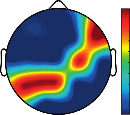

6 The Scientific World Journal

 Xn+1 � RXn 1 − Xn . (14) Table 1: The first Lyapunov exponent for logistic mapping.
 The first Lyapunov exponent
 The calculations of the first Lyapunov exponent were
 Wolf Rosenstein Sano–Sawada
carried out for R � 4. Table 1 shows the values of the first LLE: 0.99683 LLE: 0.690553 LES: 0.69317
Lyapunov exponent. As can be seen from the table, the
Rosenstein method and the Sano–Sawada method give the
closest results. Table 2: The first Lyapunov exponent for the Rössler attractor.
 The first Lyapunov exponent
3.4.2. Rössler Attractor. The Rössler differential equations Wolf Rosenstein Sano–sawada
are studied [31]: LLE: 0.05855 LLE: 0.0726 LES: 0.099851; − 0.014317; − 0.72266
 ⎪
 ⎧ x_ � − y − z,
 ⎪
 ⎨
 ⎪ y_ � x + ay, (15) Table 3: The first Lyapunov exponent for the Hénon map.
 ⎪
 ⎩
 z_ � b + z(x − c). The first Lyapunov exponent
 The calculations were performed for the parameters: Wolf Rosenstein Jacobian
 LLE: 0.38788 LLE: 0.414218 LES: 0.42703; − 1.5717
a � b � 0.2 and c � 5.7.
 Table 2 shows the first Lyapunov exponents calculated by
three methods, all of them have positive values. Also in The initial time series is divided into nonoverlapping win-
Table 2, for the Rössler attractor, the Lyapunov exponent dows of length τ, and then the values are averaged for each
spectrum is calculated by the Sano–Sawada method. window. Thus, each element of the simplified time series is
 calculated by the following formula:
 jr
 1 N
3.4.3. Hénon Map. The Hénon map [30] takes a point with y(τ)
 j � xi , 1≤j≤ . (17)
coordinates (Xn , Yn ) and maps it to a new point according τ i�(j− 1)τ +1
 τ
to the law:
 For the first scale, the time series y(1) is equivalent to
 Xn+1 � 1 − aX2n + Yn , the original time series. The length of each time series
 (16)
 Yn+1 � bXn . corresponds to the length of the original time series divided
 by the scaling parameter τ.
 The following parameters were used for the calculation: The quantitative measure calculation of entropy SE for
a � 1.4, b � 0.3. each simplified time series is carried out according to the
 Since the equations do not describe any real system, the following formula:
parameters are simply numbers. Table 3 shows the first
 N− m ′m
 i�1 ni
Lyapunov exponents calculated by three methods, all of SE (m, r, N) � ln m ′m+1 , (18)
them have positive values. The Rosenstein method and the N−
 i�1 ni
Sano–Sawada method give the closest results. Also in Table 3,
 where m is the increment of the data vector length, r is the
for Hénon map by the Sano–Sawada method, the spectrum of
 cell size in the phase space (error), and n′m
 i is the probability
Lyapunov exponents was calculated.
 of repeating a given length data sequence in the source data.
 The values of the highest Lyapunov exponent calculated
by the Rosenstein method, the Wolf method, and the
Sano–Sawada method for classical problems are in good 5. Lempel–Ziv Complexity (LZC)
agreement with each other. Along with the indicated
methods for calculating Lyapunov exponents, there is the In [38], Lempel and Ziv proposed a measure of the patterns
Kantz method [9] and the modified neural network method complexity for finite length sequences. Later, Kaspar and
[36]. It is worth noting that the calculation of the Lyapunov Schuster developed an algorithm for computing LZC on a
exponent spectrum using the modification of neural net- computer, which determined the measure of complexity
works takes a longer time compared to the Sano–Sawada [39]. LZC calculates the quantity of new images, i.e., seg-
method. Due to the fact that the Sano–Sawada method is ments that are not consistently represented in all previous
simpler to implement and takes the least time to calculate, it data. In this algorithm, the EEG signal {x(n)} is converted
is most preferable for calculating the spectrum of Lyapunov into a binary sequence {s(n)} by comparison with the av-
exponents. erage value of the signal m. After obtaining the binary se-
 quence, the corresponding measure of complexity c(n) is
 increased by one until a new sequence is detected. The
4. Multiscale Entropy (MSE)
 sequence search process is repeated until the last time the
According to the method of calculating of multiscale entropy series character has been read. LZC is defined as
(MSE) presented in [37], for a given discrete time series c(n)
 x1 , . . . , xi , . . . , xN , a sequence from the simplified time LZC � , (19)
 b(n)
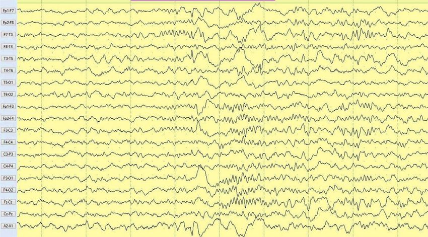
series y(τ) is determined relative to the scaling parameter τ.

The Scientific World Journal 7

 ×10–3
Le1 Le1
 3.5

 0.5
 3

 0.4 2.5

 0.3 2

 1.5
 0.2

 1
 0.1
 0.5

 0
 0
 O1
 O2
 P4
 P3
 C4
 C3
 F4
 F3
 Fp2
 Fp1
 T6
 T5
 T4
 T3
 F8
 F7
 Pz
 Cz
 Fz
 A2
 A1

 O1
 O2
 P4
 P3
 C4
 C3
 F4
 F3
 Fp2
 Fp1
 T6
 T5
 T4
 T3
 F8
 F7
 Pz
 Cz
 Fz
 A2
 A1
 Rosenstein Wolf
 Wolf
 Sano-Sawada (a) (b)

 Figure 3: First Lyapunov exponent for 2015.

 Le1 Le1
 0.5 0.06

 0.45
 0.05
 0.4
 0.35 0.04
 0.3
 0.25 0.03
 0.2
 0.02
 0.15
 0.1
 0.01
 0.05
 0 0
 2 4 6 8 10 12 14 16 18 20 2 4 6 8 10 12 14 16 18 20

 Sano-Sawada Wolf
 Rosenstein
 Wolf
 (a) (b)

 Figure 4: First Lyapunov exponent for 2018.

where b(n) � n/log2 (n). the recording of the EEG, many factors had been influencing
 the patient’s condition, including changes in therapy: a
 combination of medicaments and their doses. The study was
6. Analysis of the EEG Signals of a Patient with carried out using nonlinear dynamics methods, namely, the
 Epilepsy Using Lyapunov Exponents, Multiscale Lyapunov exponent’s analysis, multiscale entropy, and
 Entropy, and Lempel–Ziv Complexity Lempel–Ziv complexity.
 For each year under consideration, Lyapunov’s first
We study fragments of EEG signals containing pathological exponents (Le1) were calculated in each channel by three
changes in the “sharp wave” (according to the international methods: Rosenstein (blue line), Sano–Sawada (red line),
classification of EEG disorders, Luders H, Noachtar S, 2000) and Wolf (green line). Figures 3 and 4 show the results for
of the patient, who suffered from epilepsy during 2014–2019 2015 and 2018 years, respectively. The first Lyapunov ex-
in order to study the general patient condition. EEG re- ponents calculated by the Wolf and Sano–Sawada method
cordings were taken once a year in interictal periods. During are close to each other, and only in some channels the values

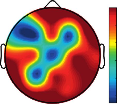
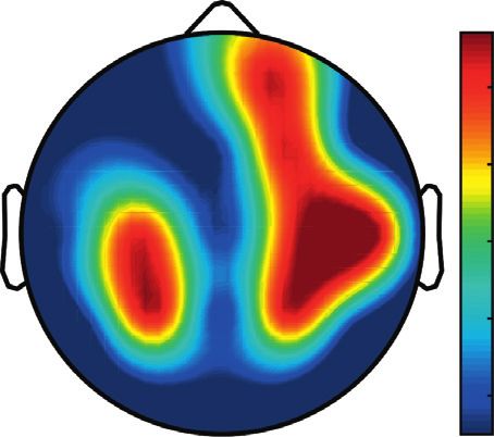
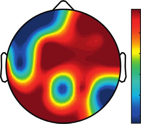
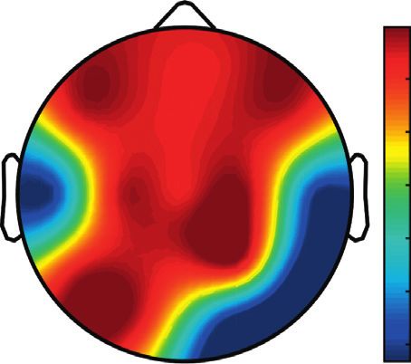
8 The Scientific World Journal

 Figure 5: EEG fragment of a patient with epilepsy.

by the Sano–Sawada and Rosenstein methods coincide. The average value of the Lyapunov exponent for all channels. In
“sharp wave” pattern on the EEG is observed in the F7 2014, a “sharp wave” pattern was observed for the patient on
channel (Figure 5), and on the charts of the first Lyapunov the EEG in the F7, T3, and F3 channels, and the response of
exponent calculated by the Rosenstein and Sano–Sawada this wave is also extended to the right hemisphere channels
method, a local minimum is reached in the F7 channel T4, T6, and O2, which is confirmed by the closeness to the
(Figures 3(a) and 4(a)). The Rosenstein method gives the zero value of the first Lyapunov exponent in these channels
widest range of values across channels [5∗ 10− 2; 6∗ 10− 1] calculated by the Rosenstein method (Table 4). Similar results
(Figures 3(a) and 4(a)). were obtained for the remaining years, and there is a tendency
 In the graph of the Lyapunov exponent calculated by to increase zones in which the Lyapunov exponent is close to
the Rosenstein method, in 2015 (Figure 3(a)), local zero, which characterizes the general deterioration of the
maxima are observed in the channels P4, C4, C3, Fp2, T6, patient’s condition. Table 4 shows the distribution of Lya-
F8, Pz, and Fz; and in 2018 (Figure 4(a)), only in the punov exponents for each channel over the scalp surface. To
channels P3, C4, T5, F8, and Pz, thus the average value visualize the obtained data in the Matlab software package,
becomes closer to zero, which characterizes the disease algorithms for constructing topographic images of Lyapunov
spread to other brain areas. Qualitatively, the distribution exponents were implemented in accordance with electrodes
of the first Lyapunov exponent over the channels, cal- arrangement in Figure 2. The values at the intermediate points
culated by the three methods, coincides. The value of the were interpolated using a spherical spline. The minimum
first Lyapunov exponent calculated by the Sano–Sawada values are shown in blue and the maximum values in dark red.
method has a negative value in some channels Consider the average across all channels of the first
(Figures 3(a) and 4(a)), which is a measure of the average Lyapunov exponent calculated by three methods: Rosenstein
exponential convergence of the trajectories to the (blue line), Sano–Sawada (red line), and Wolf (green line). Let
attractor. All this indicates a trend of worsened patient us construct the distribution diagrams over the years of the
condition. On the joint figures (Figures 3(a) and 4(a)), due obtained average value for the first Lyapunov exponent
to the smallness of the first Lyapunov exponent values (Figure 6). Qualitatively, the Sano–Sawada and Rosenstein
calculated by the Wolf method, the line corresponding to methods give similar results (Figure 6(a)). In 2015 and 2017,
it is straightened. Therefore, to see the distribution nature there are local minima (Figure 6(a)), which characterizes the
over the channels, a graph of the first Lyapunov exponent deterioration of the patient’s condition. During this period,
is calculated by the Wolf method only (Figures 3(b) and the patient had more frequent focal seizures with impaired
4(b)). The Wolf method has low sensitivity, and the first consciousness and bilateral tonic-clonic seizures resumed
Lyapunov exponent values are in the range [− 1∗ 10− 3; (Figure 1). All three methods give positive values of the first
3∗ 10− 3], that is, very close to zero. In 2018, according to Lyapunov exponent; however, the general trend in the values
the Wolf method, the first Lyapunov exponent in channel distribution from 2014 to 2019 years indicates the values tend
T3 is zero (Figure 4(b)), i.e., the signal is harmonic, and to zero (Figure 6(a)) and the Wolf method gives results very
this fact is in good agreement with the neuroimaging data close to zero throughout all years (Figure 6(b)), which in-
that the patient has structural changes in the left temporal dicates a trend towards signals “harmonization”, i.e., wors-
region. ening of the patient whole condition.
 However, it is worth noting that pathological electrical In the future, due to the fact that all three methods
activity from one brain zone extends to the remaining zones qualitatively show one trend, we will calculate the Lyapunov
and has a significant effect, so it makes sense to study the exponent spectrum by the Sano–Sawada method. It is worth

The Scientific World Journal

 Table 4: The first Lyapunov exponent in channels calculated by the Rosenstein.
2014 2015 2016 2017 2018 2019

 0.6
 0.5 0.5
 0.6 0.5 0.5 0.45
 0.5 0.4 0.4
 0.4 0.4 0.35
 0.4 0.3
 0.3 0.3
 0.3
 0.3 0.25
 0.2 0.2 0.2
 0.2 0.2
 0.15
 0.1 0.1 0.1 0.1
 0.1
 9

10 The Scientific World Journal

 ×10–3
 0.6 2.1
 Le1 Le1
 0.5 2

 1.9
 0.4
 1.8
 0.3
 1.7
 0.2
 1.6
 0.1
 1.5

 0 1.4

 –0.1 1.3
 2014 2015 2016 2017 2018 2019 2014 2015 2016 2017 2018 2019
 Sano-Sawada Wolf
 Rosenstein
 Wolf
 (a) (b)

 Figure 6: Distribution of the channel-averaged values of the first Lyapunov’s exponents by three methods for 2014–2019 years.

 Le

 0

 –0.2

 –0.4

 –0.6

 –0.8

 –1

 –1.2

 –1.4
 O1

 O2

 P4

 P3

 C4

 C3

 F4

 F3

 Fp2

 Fp1

 T6

 T5

 T4

 T3

 F8

 F7

 Pz

 Cz

 Fz

 A2

 A1

 Le1 Le5
 Le2 Le6
 Le3 Le7
 Le4

 Figure 7: The Lyapunov exponent’s spectrum according to the Sano–Sawada method for 2015.

noting that the value of the first Lyapunov exponent depends have negative values. The channel-averaged values of the
on the amount of calculated exponents in the spectrum. Lyapunov exponent’s spectrum during 2014–2019 (Figure 9)
Here are the graphs of the Lyapunov exponents spectrum tend to zero, which again indicates a deterioration in the
(Le1-Le7) calculated by the Sano–Sawada method in each patient’s condition.
channel for 2015 (Figure 7) and 2018 (Figure 8) years, as well To estimate the EEG signals complexity, we apply al-
as the spectrum distribution of the averaged Lyapunov gorithms for calculating multiscale entropy (MSE) and the
exponents over the channels for the years 2014–2019 (Fig- Lempel–Ziv complexity measure (LZC). EEG signals can be
ure 9). As can be seen from the graphs, the first Lyapunov represented at various spatial and temporal scales, so their
exponent (Le1) has a positive, but close to zero value. The complexity is also multiscale. Given this statement, MSE
remaining exponents, starting from the second, (Le2-Le7) analysis was carried out for various scales d � 2, . . . , 5 (see

The Scientific World Journal 11

 0.2
 Le

 0

 –0.2

 –0.4

 –0.6

 –0.8

 –1

 –1.2

 –1.4

 –1.6
 O1

 O2

 P4

 P3

 C4

 C3

 F4

 F3

 Fp2

 Fp1

 T6

 T5

 T4

 T3

 F8

 F7

 Pz

 Cz

 Fz

 A2

 A1
 Le1 Le5
 Le2 Le6
 Le3 Le7
 Le4

 Figure 8: The Lyapunov exponent’s spectrum by the Sano–Sawada method in 2018.

 0.2
 Le
 0

 –0.2

 –0.4

 –0.6

 –0.8

 –1
 2014 2015 2016 2017 2018 2019
 Le1 Le5
 Le2 Le6
 Le3 Le7
 Le4
Figure 9: Distribution of the channel-averaged Lyapunov exponents spectrum according to the Sano–Sawada method for the 2014–2019
years.

Figure 10(a)). The analysis of the plots of the channel-av- When calculating the Lempel–Ziv complexity (LZC),
eraged MSE value for every considered year (see normalization of values was used. A decrease in entropy and
Figure 10(a)) shows that the increase of the scaling coeffi- an increase in the Lempel–Ziv complexity characterize a
cient above d � 4 is redundant, as convergence of entropy decrease in the signal randomness. The average value graph
values is reached. Thus, the following parameters are used across all channels of the Lempel–Ziv complexity has a local
for the entropy analysis: embedding dimension m � 20, error maximum in 2015 and 2018 years (Figure 10(b)), and
r � 0.4, and scaling coefficient d � 3. multiscale entropy has a local minimum in 2016 and 2018

12 The Scientific World Journal

 0.45 0.06

 0.4
 0.055
 0.35
 0.05
 0.3
 MSE

 LZC
 0.25 0.045

 0.2
 0.04
 0.15
 0.035
 0.1

 0.05 0.03
 2014 2015 2016 2017 2018 2019 2014 2015 2016 2017 2018 2019
 d=2 d=4
 d=3 d=5
 (a) (b)

 Figure 10: Multiscale entropy (MSE) (a) and Lempel–Ziv complexity (LZC) (b) for the years 2014–2019.

(Figure 10(a)), which is well comparable with the dynamics entropy, and Lempel–Ziv complexity) showed deterioration
of patient seizures (Figure 1). In 2017, the patient experi- in the patient’s condition during the period under review,
enced remission of tonic-clonic seizures, which is in good which is in good agreement with the medical report.
agreement with the LZC graph (local minimum in 2017) and The developed software package based on the proposed
the MSE graph (local maximum in 2017). methodology can be used in the medical epilepsy diagnosis,
 as well as a qualitative therapy selection.
7. Conclusion
In the present work, for the first time, an investigation was Data Availability
made for EEG signals containing pathological changes in the
“sharp wave” for a patient with focal epilepsy for several The data used to support the findings of this study are
years using methods of nonlinear dynamics (analysis of the available from the corresponding author upon request.
spectrum of Lyapunov exponents, Lempel–Ziv complexity,
and multiscale entropy). A unified approach to the analysis Conflicts of Interest
of EEG signals based on the above methods was developed,
which can be used for the early detection of structural The authors declare that there are no conflicts of interest
changes in the brain and treatment effectiveness prediction. regarding the publication of this paper.
 For the first time, to obtain the results reliability, the
analysis of Lyapunov exponents was carried out by several Acknowledgments
different methods (Wolf, Rosenstein, and Sano–Sawada). It
was revealed that the Rosenstein method is the most in- This work was supported by the Ministry of Science and
formative for the zones localization of abnormal activity, and Education of Russian Federation (Grant 3.861.2017/4.6
the Sano–Sawada method well describes the general trend in (3.861.2017/TY))
the condition change of a patient with epilepsy. Such
characteristics as MSE and LZC are informative when References
comparing the patient’s condition in the current year with
the previous one. [1] N. V. Stankevich, A. Dvorak, V. Astakhov et al., “Chaos and
 Using the methods of nonlinear dynamics, it was hyperchaos in coupled antiphase driven toda oscillators,”
revealed that the deviations are located in the temporal parts Regular and Chaotic Dynamics, vol. 23, no. 1, pp. 120–126,
of the hemispheres, which advise the channels T3 and T4. 2018.
This is confirmed by high-resolution brain MRI according to [2] J. Awrejcewicz, V. A. Krysko, I. V. Papkova, and A. V. Krysko,
the epileptological program: structural changes in the “Deterministic chaos in one-dimensional continuous sys-
 tems,” in World Scientific, Singapore, 2016.
temporal region were revealed in the form of a combination
 [3] A. V. Krysko, J. Awrejcewicz, A. A. Zakharova, I. V. Papkova,
of focal cortical dysplasia of the left temporal lobe medi- and V. A. Krysko, “Chaotic vibrations of flexible shallow
obasal parts and left hippocampal sclerosis, as well as axially symmetric shells,” Nonlinear Dynamics, vol. 91, no. 4,
metabolic disorders of the right hippocampus. pp. 2271–2291, 2018.
 The results obtained using the proposed methodology [4] V. A. Krysko, J. Awrejcewicz, M. V. Zhigalov,
(analysis of the Lyapunov exponents spectrum, multiscale V. F. Kirichenko, and A. V. Krysko, “Mathematical models

The Scientific World Journal 13

 ofhigher orders,” Shells in Temperature Fields, Berlin, Ger- [20] M. Sano and Y. Sawada, “Measurement of Lyapunov spec-
 many, Springer, Berlin, Germany, p. 447, 2019. trum from a chaotic time series,” Physical Review Letters,
 [5] T. Y. Yaroshenko, D. V. Krysko, V. Dobriyan et al., “Wavelet vol. 55, no. 10, pp. 1082–1085, 1985.
 modeling and prediction of the stability of states: the Roman [21] E. Ubeyli and I. Guler, “Statistics over Lyapunov exponents for
 Empire and the European Union,” Communications in feature extraction: electroencephalographic changes detection
 Nonlinear Science and Numerical Simulation, vol. 26, no. 1–3, case,” Engineering and Technology, vol. 2, pp. 132–135, 2005.
 pp. 265–275, 2015. [22] B. N. Datta, V. A. Yatsenko, and S. P. Nair, “Model updating and
 [6] B. Swiderski, S. Osowski, and A. Rysz, “Lyapunov exponent of simulation of Lyapunov exponents,” in Proceedings of the Euro-
 EEG signal for epileptic seizure characterization,” in Pro- pean Control Conference, pp. 1094–1100, Kos, Greece, July 2007.
 ceedings of the 2005 European Conference on Circuit Theory [23] A. Das, P. Das, and A. B. Roy, “Applicability of Lyapunov
 and Design, Cork, Ireland, Novermber 2005. exponent in EEG data analysis,” Complexity International,
 [7] S. Osowski, B. Swiderski, A. Cichocki, and A. Rysz, “Epileptic vol. 9, pp. 1–8, 2002.
 seizure characterization by Lyapunov exponent of EEG sig- [24] A. Das, P. Das, and A. B. Roy, “Nonlinear data analysis of
 nal,” COMPEL: The International Journal for Computation experimental (EEG) data and comparison with theoretical
 and Mathematics in Electrical and Electronic Engineering, (ANN) data,” Complexity, vol. 7, no. 3, pp. 30–40, 2002.
 vol. 26, no. 5, pp. 1276–1287, 2007. [25] A. Aarabi and B. He, “Seizure prediction in patients with focal
 [8] V. Golovko, S. Artsiomenka, V. Kisten, and V. Evstigneev, hippocampal epilepsy,” Clinical Neurophysiology, vol. 128,
 “Towards automatic epileptic seizure detection in EEGs based no. 7, pp. 1299–1307, 2017.
 on neural networks and largest Lyapunov exponent,” Inter- [26] J. Hu, J. Gao, and J. C. Principe, “Analysis of biomedical
 national Journal of Computing, vol. 14, no. 1, pp. 36–47, 2015. signals by the Lempel-Ziv complexity: the effect of finite data
 [9] H. Kantz, “A robust method to estimate the maximal Lya- size,” IEEE Transactions on Bio-Medical Engineering, vol. 53,
 punov exponent of a time series,” Physics Letters A, vol. 185, no. 12, pp. 2606–2609, 2006.
 no. 1, pp. 77–87, 1994. [27] J. Gao, J. Hu, and W.-W. Tung, “Complexity measures of
[10] N. Mammone, J. C. Principe, F. C. Morabito, D. S. Shiau, and brain wave dynamics,” Cognitive Neurodynamics, vol. 5, no. 2,
 J. C. Sackellares, “Visualization and modelling of STLmax pp. 171–182, 2011.
 topographic brain activity maps,” Journal of Neuroscience [28] Y. Yin, K. Sun, and S. He, “Multiscale permutation Rényi
 Methods, vol. 189, no. 2, pp. 281–294, 2010. entropy and its application for EEG signals,” PLoS One,
[11] N. Mammone, F. C. Morabito, and J. C. Principe, “Visu- vol. 13, no. 9, Article ID 0202558, 2018.
 alization of the short term maximum lyapunov exponent [29] R. May, “Simple mathematical model with very complicated
 topography in the epileptic brain,” in Proceedings of the dynamics,” Nature, vol. 261, pp. 459–467, 1976.
 2006 International Conference of the IEEE Engineering in [30] M. Hénon, “A two-dimensional mapping with a strange
 Medicine and Biology Society, New York, NY, USA, August attractor,” Communications in Mathematical Physics, vol. 50,
 2006. no. 1, pp. 69–77, 1976.
[12] A. Wolf, J. B. Swift, H. L. Swinney, and J. A. Vastano, “De- [31] H.-O. Peitgen, H. Jürgens, and D. Saupe, 12.3 The Rössler
 termining Lyapunov exponents from a time series,” Physica D: Attractor, «Chaos and Fractals: New Frontiers of Science»,
 Nonlinear Phenomena, vol. 16, no. 3, pp. 285–317, 1985. pp. 636–646, Springer, Berlin, Germany, 2004.
[13] L. D. Iasemidis and J. C. Sackellares, “The evolution with time [32] A. O. Lpmnp[prpc, “Pb ;otrpVjj oa fejojxu crfnfoj
 of the spatial distribution of the largest Lyapunov exponent on lal nftrjyfslpn jocarjaotf actpnprvjinpc,” EAO
 the human epileptic cortex,” in Measuring Chaos in the SSSR, vol. 124, pp. 754-755, 1959.
 Human Brain, D. W. Duke and W. S. Pritchard, Eds., [33] 6. Γ. Sjoak, “P Vpo>tjj ;otrpVjj ejoanjyfslpk
 pp. 49–82, World Scientific, Singapore, 1991. sjstfn9,” EAO SSSR, vol. 124, pp. 768–771, 1959.
[14] L. D. Iasemidis, On the dynamics of the human brain in [34] J.-P. Eckmann and D. Ruelle, “Ergodic theory of chaos and
 temporal lobe epilepsy, Ph.D. dissertation, University of strange attractors,” Reviews of Modern Physics, vol. 57, no. 3,
 Michigan, Ann Arbor, MI, USA, 1991. pp. 617–656, 1985.
[15] S. P. Nair, D.-S. Shiau, J. C. Principe et al., “An investigation of [35] S. Sato, M. Sano, and Y. Sawada, “Practical methods of
 EEG dynamics in an animal model of temporal lobe epilepsy measuring the generalized dimension and the largest Lya-
 using the maximum Lyapunov exponent,” Experimental punov exponent in high dimensional chaotic systems,”
 Neurology, vol. 216, no. 1, pp. 115–121, 2009. Progress of Theoretical Physics, vol. 77, no. 1, pp. 1–5, 1987.
[16] N. Guler, E. Ubeyli, and I. Guler, “Recurrent neural networks [36] J. Awrejcewicz, A. Krysko, N. Erofeev, V. Dobriyan,
 employing Lyapunov exponents for EEG signals classifica- M. Barulina, and V. Krysko, “Quantifying chaos by various
 tion,” Expert Systems with Applications, vol. 29, no. 3, computational methods. Part 1: simple systems,” Entropy,
 pp. 506–514, 2005. vol. 20, no. 3, p. 175, 2018.
[17] E. D. Av, “Lyapunov exponents/probabilistic neural networks [37] S. H. Na, S. H. Jin, S. Y. Kim, and B.-J. Ham, “EEG in
 for analysis of EEG signals,” Expert Systems with Applications, schizophrenic patients: mutual information analysis,” Clinical
 vol. 37, no. 2, pp. 985–992, 2010. Neurophysiology, vol. 113, no. 12, pp. 1954–1960, 2002.
[18] T. Q. D. Khoa, N. T. M. Huong, and V. V. Toi1, “Detecting [38] A. Lempel and J. Ziv, “On the complexity of finite sequences,”
 epileptic seizure fromScalp EEG using Lyapunov spectrum,” IEEE Transactions on information theory, vol. 22, pp. 75–81, 1976.
 Computational and Mathematical Methods in Medicine, [39] F. Kaspar and H. G. Schuster, “Easily calculable measure for
 vol. 2012, Article ID 847686, 11 pages, 2012. the complexity of spatiotemporal patterns,” Physical Review
[19] M. T. Rosenstein, J. J. Collins, and C. J. de Luca, “A practical A, vol. 36, no. 2, 1987.
 method for calculating largest Lyapunov exponents from
 small data sets,” Physica D: Nonlinear Phenomena, vol. 65,
 no. 1-2, pp. 117–134, 1993.