Evaluation of Dynamic Cointegration-Based Pairs Trading Strategy in the Cryptocurrency Market
←
→
Page content transcription
If your browser does not render page correctly, please read the page content below
Evaluation of Dynamic Cointegration-Based Pairs
                                             Trading Strategy in the Cryptocurrency Market
                                                                               M ASOOD TADI
                                                              CY Tech, CY Cergy Paris University, Cergy, France
                                                                          tadimasood@cy-tech.fr

                                                                           I RINA KORTCHEMSKI
                                                              CY Tech, CY Cergy Paris University, Cergy, France
arXiv:2109.10662v1 [q-fin.TR] 22 Sep 2021

                                                                                  ik@cy-tech.fr

                                            Abstract
                                            Purpose — This research aims to demonstrate a dynamic cointegration-based pairs
                                            trading strategy, including an optimal look-back window framework in the
                                            cryptocurrency market, and evaluate its return and risk by applying three different
                                            scenarios.
                                            Design/methodology/approach — We employ the Engle-Granger methodology, the
                                            Kapetanios-Snell-Shin (KSS) test, and the Johansen test as cointegration tests in
                                            different scenarios. We calibrate the mean-reversion speed of the Ornstein-Uhlenbeck
                                            process to obtain the half-life used for the asset selection phase and look-back window
                                            estimation.
                                            Findings — By considering the main limitations in the market microstructure, our
                                            strategy exceeds the naive buy-and-hold approach in the Bitmex exchange. Another
                                            significant finding is that we implement a numerous collection of cryptocurrency coins
                                            to formulate the model’s spread, which improves the risk-adjusted profitability of the
                                            pairs trading strategy. Besides, the strategy’s maximum drawdown level is reasonably
                                            low, which makes it useful to be deployed. The results also indicate that a class of
                                            coins has better potential arbitrage opportunities than others.
                                            Originality/value — This research has some noticeable advantages, making it stand out
                                            from similar studies in the cryptocurrency market. First is the accuracy of data in which
                                            minute-binned data create the signals in the formation period. Besides, to backtest the
                                            strategy during the trading period, we simulate the trading signals using best bid/ask
                                            quotes and market trades. We exclusively take the order execution into account when
                                            the asset size is already available at its quoted price (with one or more period gaps after
                                            signal generation). This action makes the backtesting much more realistic.

                                                                                        1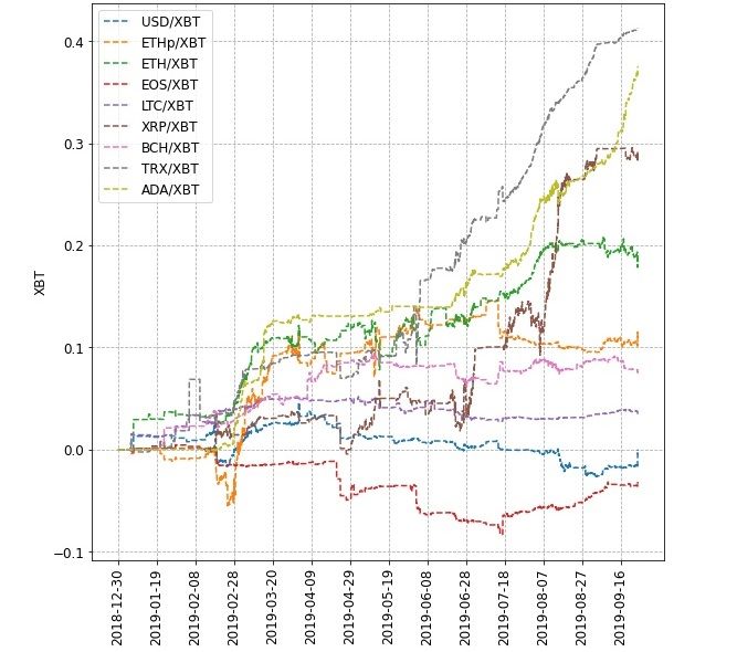
Keywords — Arbitrage opportunity, Pairs trading strategy, Basket trading,
Cointegration, Mean reversion, Cryptocurrency market
Paper type — Research paper

                                   2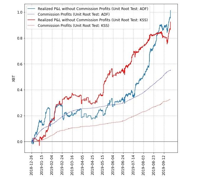
1    Introduction
A cryptocurrency is volatile digital security designed to operate as a tool of exchange
that uses secure cryptography (Gandal and Halaburda 2016). Bitcoin is the first
cryptocurrency that is issued in 2009. After the bitcoin announcement, a lot of
alternative cryptocurrencies (altcoins) have been created.           The total market
capitalization of the cryptocurrency market is more than 341 billion dollars on
30/09/2020 (See Coinmarketcap.com). Deploying algorithmic trading strategies is
developing over time in the Cryptocurrency market, accelerating tradings to maximize
profits.
One of the most well-known strategies among different algorithmic trading methods is
the statistical arbitrage strategy. Statistical arbitrage is a profitable situation stemming
from pricing inefficiencies among financial markets. Statistical arbitrage is not a real
arbitrage opportunity, but it is merely possible to obtain profit applying past statistics
(Aldridge 2013). In fact, there are two different potential arbitrage opportunities in the
cryptocurrency market; the exchange to exchange arbitrage and the statistical arbitrage.
The exchange to exchange arbitrage has a potential profit, but it is quite risky, and there
are many challenges to deploy it. Instead, the statistical arbitrage opportunities have the
same potential profits without the same risks as the former one (Pritchard 2018).
Statistical arbitrage strategies are often deployed based on mean reversion property, but
they can also be designed using other factors. Pairs trading is the commonly recognized
statistical arbitrage strategy that involves identifying pairs of securities whose prices
tend to move mutually. Whenever the relationship between financial securities behaves
abnormally, the pair would be traded. Then the open positions will be closed when the
unusual behavior of pairs reverts to their normal mode (Vidyamurthy 2004).
According to Krauss (2017), pairs trading strategy is a two-step process. The first step,
which is called the formation period, attempts to find two or more securities whose
prices move together historically. In the second step, which is the trading period, we
seek abnormalities with their price movement to profit from statistical arbitrage
opportunities.
There are two general approaches to find appropriate pairs of assets in the formation
period: the heuristic approach and the statistical approach. The heuristic approach,
which is regularly called the distance approach, is more straightforward than the
statistical approach, which the latter is based on the cointegration concept. In the
trading period, we can combine our strategy with different mathematical tools such as
stochastic processes, stochastic control, machine learning, and other methods to
improve the results (ibid.).
Compared to the leading financial markets, such as the stock market and fixed income
market, limited research has been conducted on statistical arbitrage strategies in the

                                             3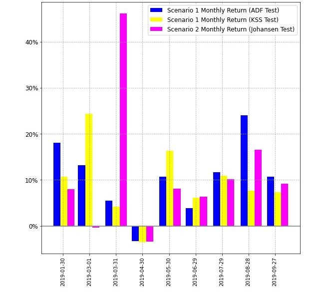
cryptocurrency market. In the next section, we review some papers concerning these
strategies frequently studied in the cryptocurrency market and explain some of their
practical weaknesses and drawbacks.

2    Literature Review
The distance approach is the basic researched framework introduced by Gatev,
Goetzmann, and Rouwenhorst (2006). This method is based on the minimum squared
distance of the normalized price of assets. The distance between normalized prices is
called spread. In order to construct a measurable scale, assets should become normal
first. To this aim, asset prices are divided into their initial value, and then the spread is
obtained by taking the difference between normalized prices. In the formation period,
the top first pairs with the minimum historic sum of squared distances between
normalized prices are considered in a subsequent trading period (ibid.).
According to Perlin (2009), the price series can be normalized first based on their
historical mean and historical volatility, and then the spread of each pair can be
constructed in the same way. Finally, in the trading period, the pairs arranged in their
ascending orders can be picked using the top first pairs of the list for pairs formation.
Simple non-parametric threshold rules are used to trigger trading signals. This
threshold and can be two historical standard deviations of normalized spread price.
The main findings establish distance pairs trading as profitable across different markets,
asset classes, and time frames. Driaunys et al. (2014) studied a pairs trading strategy
at the natural gas futures market based on the distance approach. In their research,
pairs of two futures contracts of the same underlying asset are selected, i.e., natural gas
with different maturities, which are the most liquid, close to expiration, and therefore
they are correlated contracts of natural gas futures. The contract with bid prices is
shorted through the trading period, Whenever the distance of the given d is reached.
Besides, the long position of the contract with the asking price is taken. They backtest
their model with different moving windows and different thresholds and realize that the
higher values of d works better and generate fewer trades and make the model more
stable.
Driaunys et al. (ibid.)’s research has some weaknesses in practice. First, the assumption
of no transaction cost makes their result unreliable. Second, they did not calculate the
risk-adjusted return of different scenarios. So, the performance of the research’s strategy
is questionable. Furthermore, they did not compare their method with a naive strategy,
i.e., buy-and-hold strategy, and besides, the required investment to deploy the strategy
is not determined.
Other researches are based on the statistical approach. This approach identifies two

                                             4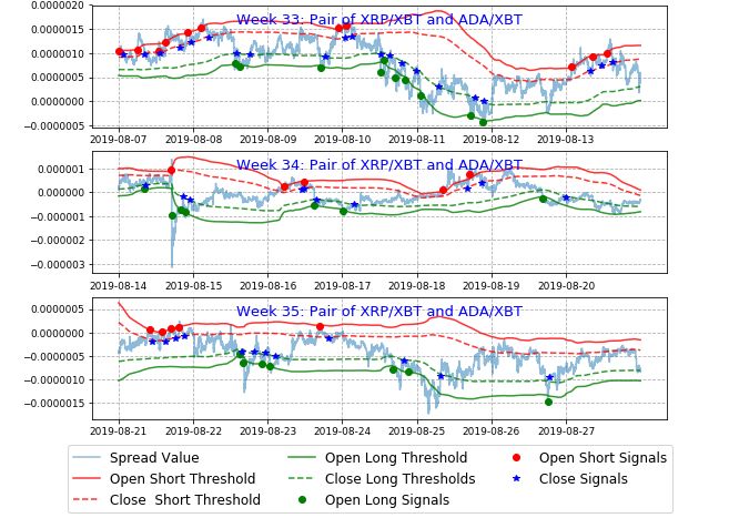
or more time-series combined to form a long-term equilibrium relationship, although
the time series themselves may have a non-stationary trend. There are some research
papers based on the cointegration concept in the cryptocurrency market. Broek and
Sharif (2018) selected a set of cryptocurrency coins and split them into four main sectors
that depend on the coins’ fundamental features. Then, by examining unit-root tests,
they achieved a cointegration relationship among coins in each group. Finally, they
concluded that implementing a pairs trading strategy could be profitable due to arbitrage
opportunities. Nevertheless, ignoring the transaction costs and having a bias selection
make this paper’s profitability results unreliable.
Leung and Nguyen (2019) constructed cointegrated cryptocurrency pairs using three
different unit-root tests. Using the daily prices of four cryptocurrency coins from
Coinbase exchange, they introduced the ordinary least squares model to build a
cointegrated combination of coins and set the p-values of the estimated coefficients
less than 1%. The authors backtested the strategy with five different entry/exit
threshold levels. They realized that with the threshold set at 1.5 standard deviation, the
strategy is optimal. Furthermore, they incorporated the stop-loss exit and trailing
stop-loss exit possibilities, which lowered the profit return.
Kakushadze and Yu (2019) proposed the momentum factor statistical arbitrage
methodology based on a dollar-neutral mean-reversion strategy. Their method is to
short a fixed level of Bitcoin and keep it throughout the trading period and long
multiple altcoins, which varies every day depending on their momentum values. They
realized that low liquid altcoins have a better mean-reverting feature. Furthermore,
they found that if yesterday’s momentum of an altcoin is positive, it is expected to
trade it higher today and vise versa.
Pritchard (2018) built the strategy based on statistical tests as well as technical analysis
indicators. He applied different statistical tests such as the augmented Dickey-Fuller
test, the Hurst exponent, and the Johansen test. He achieved that each coin is not
mean-reverting, but a linear mean-reverting strategy can be implemented by
constructing the normalized deviation of price from its moving average. In his study,
the volume is considered the most critical barrier to utilize arbitrage opportunities in
the cryptocurrency market.

3    Market Structure
Numerous cryptocurrency exchanges allow their customers to trade cryptocurrencies
against other assets, such as conventional fiat money or other digital currencies.
BitMEX is one of the most well-known cryptocurrency exchanges with a Peer-to-Peer
Trading Platform, which offers leveraged contracts bought and sold in Bitcoin. This

                                             5
exchange only handles Bitcoin. All profit and loss are in Bitcoin, even if altcoins are
traded. BitMEX does not handle fiat currencies. Therefore, in order to calculate profit
and loss, we denominate all coins by Bitcoin. BitMEX offers Futures and Perpetual
Contracts and allows trading with a high amount of leverage depending on the type of
contracts. BitMEX offers perpetual swaps that have an inverse or Quanto payout. It
also offers futures contracts that have an inverse, Quanto, or linear payout. See BitMEX
exchange perpetual and futures contracts guide (accessed 2020-09-30) for more
details.
Symbol Description
XBT/USD Bitcoin/US Dollar (Inverse) Perpetual Swap
ETH/USD Ethereum Quanto Perpetual Contract
ETH/XBT Ethereum/Bitcoin Futures Contract
EOS/XBT EOS Token/Bitcoin Futures Contract
LTC/XBT Litecoin/Bitcoin Futures Contract
XRP/XBT Ripple/Bitcoin Futures Contract
BCH/XBT Bitcoin Cash/Bitcoin Futures Contract
TRX/XBT Tron/Bitcoin Futures Contract
ADA/XBT Cardano/Bitcoin Future Contract
Table I: BitMEX contracts used in the research
BitMEX uses the following industry-standard month codes to name its Futures coins.
The month code implies the delivery month of the Futures contract.
Month Code Month Month Code Month
F Jan N Jul
G Feb Q Aug
H Mar U Sep
J Apr V Oct
K May X Nov
M Jun Z Dec
Table II: Futures Expiration Month Codes on BitMEX
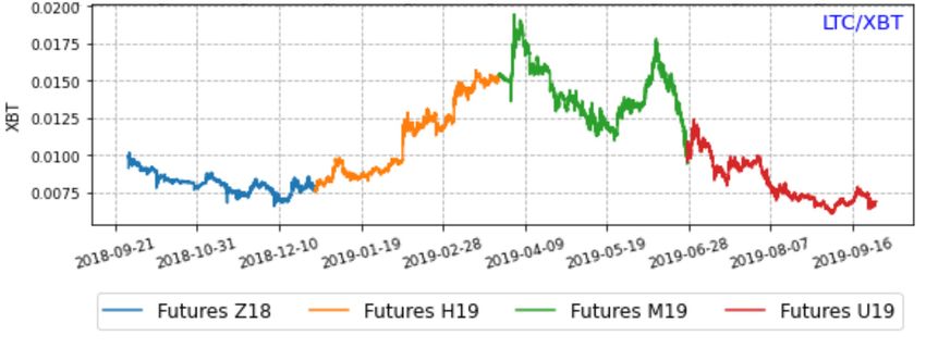
Each Futures contract is traded in three months period. In this research, the delivery
date of futures contracts are Z18, H19, M19, and U19. The letters are the expiration
month code, and the numbers show the expiration year. For instance, Litecoin has four
different delivery dates: LTCZ18, LTCH19, LTCM19, and LTCU19.
6Figure 1: LTC/XBT futures contract price during the study period
Bitcoin perpetual swap on BitMEX (XBT/USD) is a derivative product whose
underlying asset is Bitcoin in the US dollar. Since Bitcoin’s price in the US dollar is
different in each cryptocurrency exchange, Bitmex identifies an index named BXBT,
which calculates a weighted average Bitcoin price in the US dollar using several
exchanges data sources. Each Bitcoin perpetual swap contract is worth 1 USD of
Bitcoin. Note that both underlying and swap contracts are quoted in USD, but margin
and P&L are denominated in Bitcoin. It means that opening a long position of
XBT/USD is equal to open a short position of the US dollar, which is denominated in
Bitcoin. See BitMEX exchange perpetual and futures contracts guide (accessed
2020-09-30) for more details.
Figure 2: XBT/USD perpetual swap price during the study period
When we long or short a contract, there are two fundamental execution options:
placing the market order or the limit order. Market orders are executed immediately at
the market price of an asset. Conversely, in limit orders, we set a specific price that we
desire to trade. Hence there is no guarantee to have executed trades. The main
difference between these two orders is their transaction fees. Taker fees (market orders
fees) typically have a higher charge than maker fees (limit orders). In BitMEX
7exchange, maker fees for Perpetual and Futures contracts are negative (−0.0250%),
which means that by executing a limit order, we are not charged and can earn profit due
to the negative transaction fees. Taker fee is 0.0750% for all contracts. Besides, in
order to match the transaction price of a perpetual contract with its underlying coin
price, there is another fee, called funding fee which is exchanged between long and
short positions every 8 hours. Funding fee is ±0.0100% for XBT/USD and ETH/USD
perpetual contracts.
There are also other execution orders in BitMEX such as stop-loss orders, trailing stop-
loss orders, and take profit orders. The stop-loss order and trailing stop-loss order place
a market/limit order to close a position to restrict an investor’s loss on a cryptocurrency
position. On the other hand, the take profit order places a market/limit order to exit the
trade to maximize investor’s profit in unstable or bubble periods. As Geuder, Kinateder,
and Wagner (2019) studied Bitcoin price dynamics, the cryptocurrency coins (Bitcoin,
in their paper) have remarkable bubbles in specific periods. However, in other periods,
their used methodologies did not identify any bubble behavior. To overcome high risky
periods of bubble behavior of cryptocurrency coins, we can use these kinds of orders to
protect our investment and decrease the maximum drawdown of the strategy.
4 Data Source
To implement the statistical arbitrage strategy, we obtain historical minute-binned
trading data of cryptocurrency coins using the BitMEX application programmable
interface (API) from September 27, 2018, to October 2, 2019. The data consist of the
trade’s close price and the volume of each coin as well as best bid/ask quotes. We used
the data in two steps. First, for each coin, the minute-binned close price is used to
calculate cointegration tests, making a spread, calibrating half-life of the spread, and
creating trading signals of the strategy. Second, to backtest the strategy, we simulate
the orders by updating best bid/ask quotes and comparing them with market trades.
The data splitting step is dynamic. In order to create trading signals, we need to specify
a formation period to estimate our parameters. The formation period includes
three-month price data of coins. After calibrating the parameters, we start trading for
one week, corresponding to the estimated parameters. The first trading week starts on
26/12/2018. As shown in figure 3, after the first trading week, we update the formation
period and move the time horizon ahead. There are thirty-nine trading weeks in which
the last one starts from 18/09/2019.
The strategy is programmed by Python3 language and its helpful libraries such as
Pandas, Numpy, Multiprocessing, Matplotlib, Statsmodels, and Arch. We also used R
packages to perform nonlinear cointegration tests. The data is stored on Amazon Web
8Service (AWS) cloud server. To optimize the running time and facilitate programming,
we worked on JupyterLab in the Amazon SageMaker platform.
Figure 3: Dynamic Formation-Trading Periods
5 Theoretical Framework of the Strategy
This section explains the theoretical concepts, such as statistical tests and calibration
procedures required to develop our methodology.
5.1 Non-Stationary Processes and Unit-Root Test
Generally, financial variables are regularly non-stationary, which means that the data
parameters change over time. This phenomenon makes us utilize cointegration property.
If we have a collection of non-stationary time series with the same order of integration,
denoted I(d), and if a linear combination of them is stationary, then the collection is
cointegrated. Random walks are well-known examples of non-stationary processes that
can have drift and deterministic trend.
In a statistical arbitrage strategy, we create a combination of two or more assets in which
some of them are on the buy-side, and some others are on the sell-side. This combination
is called the assets spread. The methodology of formulating that spread is discussed in
section 6. Suppose that St is the spread time series. Using unit-root tests, we check if St
is a non-stationary process. In this research, the spread process is formulated such that
9the unit-root test is viewed without drift or a trend as it should revert to zero as follows
St = φ1 St−1 + t , (1)
where t indicates the error term. Consider the null hypothesis H0 : φ1 = 1 versus the
alternative hypothesis H1 : φ1 < 1. In this case, if the series St is stationary, it tends to
return to a zero mean. The Dickey–Fuller (DF) test statistic is the t ratio estimation of
the least-squares of φ1 (Tsay 2010). In general, it is easier to test a null hypothesis that
a coefficient is equal to zero, St−1 is subtracted from both sides of equation 1, to obtain
∆St = St − St−1 = γ1 St−1 + t , (2)
where γ1 = φ1 − 1. This model can be estimated and testing for a unit-root is equivalent
to testing γ1 = 0. The corresponding null and alternative hypotheses are now H0 : γ1 =
0 against H1 : γ1 < 0. Now we extend the price time series to lags more than one such
that
St = φ1 St−1 + φ2 St−2 + · · · + φp St−p + t , (3)
This series is stationary if the roots of the polynomial mp − mp−1 a1 − mp−2 a2 − · · · − ap
are all less than one in absolute value.
Pp In this case, One is a root of this polynomial if
1 − φ1 − φ2 − · · · − φk = 0 =⇒ i=1 φi = 1. Note that when p = 2 we can re-write
an the price process as follows
St = φ1 St−1 + φ2 St−2 + t
= φ1 St−1 + φ2 St−1 − φ2 St−1 + φ2 St−2 + t (4)
= (φ1 + φ2 )St−1 + γ∆St−1 + t
where γ = f (φ2 ). In general we can rewrite price process as follows
p
!
X
St = φi St−1 + γ1 ∆St−1 + · · · + γp−1 ∆St−p+1 + t (5)
i=1
Pp
where γi is f (φi+1 , · · · , φp ). By defining β = i=1 φi , the equation is
St = βSt−1 + γ1 ∆St−1 + · · · + γp−1 ∆St−p+1 + t (6)
To verify the existence of a unit-root in a spread process, one may perform the test
H0 : β = 1 vs. Ha : β < 1. This test is the augmented Dickey–Fuller (ADF) unit-
root test (Dickey and Fuller 1979). If coefficient p-value < α, we reject unit-root
non-stationary time series with (1 − α)% of statistical confidence and if coefficient
p-value ≥ α, we cannot reject unit-root non stationary time series with (1 − α)% of
statistical confidence (Tsay 2010).
10The primary point in the Dickey-Fuller test is that we assume the spread of the pairs
trading strategy is a linear Auto-regressive time series. We can extend equation 3 to
Piece-wise nonlinear time series which is called Threshold Auto-Regressive (TAR)
model such that
(
φ11 St−1 + φ12 St−2 + · · · + φ1p St−p + t , zt−d c
where zt is the transition variable, d is the delay of the transition variable, c is the
threshold of the model, and t indicates the error term. Equation 7 is a two regime TAR
model but theoretically, the number of regimes can be more than two. If zt−d = St−d ,
then The switch from one regime to another regime depends only on the past values
of the St . In this case the model is named Self-Exciting Threshold Auto-Regressive
(SETAR) model. Enders and Siklos (2001) proposed a three-step method to identify
whether there exists cointegration among time series in which their residuals (St ) are
formed by the SETAR model. They developed their method both when c is known
(c = 0) and when it is unknown. We also demonstrated that their test has greater power
compared to the Engle-Granger test when zt−d = ∆St−d . Now, We generate three
regime TAR model with one inner regime and two outer regimes as follows
φ11 St−1 + φ12 St−2 + · · · + φ1p St−p + t , zt−d < c
St = φ21 St−1 + φ22 St−2 + · · · + φ2p St−p + t zt−d = c (8)
φ31 St−1 + φ32 St−2 + · · · + φ3p St−p + t , zt−d > c
K. S. Chan et al. (1985) proved that the inner regime of equation 8 can be non-stationary
while the entire process can be globally stationary. Hence, a unit root in the inner regime
does not influence the stationarity of the entire process and we can replace the inner
regime by St−1 + t . Assume that φ1i = φ3i for i = 1, · · · , p (which means that the
SETAR model is symmetric), we deduce
(
St−1 + t zt−d = c
St = (9)
φ11 St−1 + φ12 St−2 + · · · + φ1p St−p + t , zt−d 6= c
By aassuming zt−d = St−d , and d = 1, the equation 7 can be written in the form of
indicator function as follows
p
!
St = St−1 1 − 1{St−1 6=c} + φ1i St−i 1{St−1 6=c} + t
X
i=1
p
(10)
γ1i 1{St−1 6=c} St−i + t
X
= St−1 +
i=1
11where γ1i = φ1i − 1. The transition from one regime to another in the TAR and SETAR
models are discontinuous. Hence, when c is unknown, the analytical form to obtain an
estimator for c cannot be obtained. The overcome this issue, the 1(.) is replaced by a
continuous function to have a higher level of flexibility in the model. So the Smooth
Transition Auto-regressive (STAR) model is
p
X
St = St−1 + (γ1i G(St−1 ; θ, c) St−i ) + t (11)
i=1
where
2
G(St−1 ; θ, c) = 1 − e−θ(St−1 −c) . (12)
Equations 11 and 12 generate an Exponential Smooth Transition Auto-Regressive
(ESTAR) model. In this model, 0 ≤ G(St−1 ; θ, c) ≤ 1. For simplicity, in the case of
p = 1, and c = 0, ESTAR(1) is considered as
St = (1 + γ1 G(St−1 ; θ)) St−1 + t (13)
which can be demonstrated as
2
−θSt−1
∆St = γ1 1 − e St−1 + t (14)
Kapetanios, Shin, and Snell (2003) (hereafter KSS) presented a test for nonstationarity
with the alternative hypothesis of nonlinear stationarity. They showed that St is globally
stationary when θ > 0 and −2 < γ < 0. The null hypothesis and its alternative
hypothesis are H0 : θ = 0 and H1 : θ > 0. The problem is that γ is not identified under
the null hypothesis. In order to overcome this problem, they suggested to take first-order
Taylor approximation of the G(St−1 ; θ). Suppose that G(St−1 ; θ) = 1 − f (St−1 ; θ). The
Taylor approximation of f (θ) at θ = 0 is
∂f (f (St−1 ; θ|θ = 0)
f (St−1 ; θ) = f (St−1 ; θ|θ = 0) + (θ − 0) + C
∂θ (15)
2
= 1 − θ (St−1 ) + C
where C is the further orders of the approximation. Now, the first order Taylor
approximation of G(St−1 ; θ) at θ = 0 is θ (St−1 )2 . By replacing this expression into
equation 14 we obtain
∆St = γ1 θ (St−1 )2 St−1 + ∗t = δ (St−1 )3 + ∗t (16)
where δ = γ1 θ and ∗t = −(γ1 yt−1 )C + t . The null hypothesis and alternative
hypothesis of KSS test are now H0 : δ = 0 and H1 : δ < 0. See Kapetanios, Shin, and
Snell (2006), Kapetanios, Shin, and Snell (2003), and Patterson (2012) for more details
about KSS test characteristics.
12Finally, to test the cointegration test among multiple assets, we need to utilize the
Johansen (1991) test, a procedure for testing the cointegration of several non-stationary
time series. This test permits more than one cointegration relationship, so it is more
generally applicable than the Engle and Granger (1987) test based on the Dickey-Fuller
(or the augmented) test for unit-roots in the residuals from a single (estimated)
cointegration relationship. Like a unit-root test, suppose that we have an
auto-regressive process with order p, which is now in vector shape, named VER(p)
model. We assume that there is no trend term
St = Π0 + Π1 St−1 + · · · + Πp St−p + εt , t = 1, . . . , T. (17)
Like the augmented Dickey-Fuller test, we rewrite the spread process by differencing
the series we obtain
∆St = Π0 + ΠSt−1 − Γ1 ∆St−1 − · · · − Γp−1 ∆St−p+1 + εt , t = 1, · · · , T (18)
where Γi = (Πi+1 + · · · + Πp ) , i = 1, . . . , p − 1, and Π = Π1 + · · · + Πp − I.
∆St = St − St−1 is the difference operator, Π and Γi are the coefficient matrix for the
lags. Cointegration occurs when the matrix Π = 0. We decompose the eigenvalue of
Π. Suppose that the rank of Π is equal to r. The Johansen test’s null hypothesis is
H0 : r = 0 indicates no cointegration at all. A rank H1 : r > 0 means a cointegration
relationship within two or perhaps more time series. In this test, we sequentially test
whether r = 0, 1, p − 1, where p is the number of time series under test. Finally we find
coefficients of a linear combination of time series to produce a stationary portfolio of
time series.
5.2 Mean Reverting Processes and Half-Life Calibration
Mean reverting processes are widely observed in the financial markets. Toward mean
reverting processes, as opposed to the trend following time series, we assume that a
combination of assets tends to return to its mean level over time. A mean-reverting time
series can be interpreted by Uhlenbeck and Ornstein (1930) model or Vasicek (1977)
model, a particular case of the Hull and White (1990) model with constant volatility. It
is also the continuous-time equivalent of the discrete-time Auto-Regressive process with
order 1. The Ornstein-Uhlenbeck model specifies the stochastic differential equation as
follows
dSt = θ(µ − St ) dt + σ dWt (19)
where S0 = s0 is a known value, θ > 0, µ > 0. Wt denotes the Wiener process. In
this model, µ is the long term spread mean, θ is the mean reversion speed, and σ is the
spread’s instantaneous volatility. We rearrange the equation 19, multiply the integrating
13factor of eθt and integrate both sides knowing eθt dSt + eθt θSt dt = d(eθt St ) as follows
Z t=T Z T Z T
θt θt
d(e St ) dt = e θµ dt + eθt σ dWt (20)
t=s s s
So we obtain Z T Z T
θT θs θt
e ST − e Ss = e θµ dt + eθt σ dWt . (21)
s s
Solving for ST we get
Z T
−θ(T −s) −θ(T −s) −θT
ST = e Ss + µ(1 − e ) + σe eθt dWt (22)
s
where the expected value of St is
E[St |s0 ] = s0 e−θt + µ(1 − e−θt ). (23)
Concerning the equation 23, we can define its half-life. Half-life (t1/2 ) is the expected
time required for any quantity to decrease to half of its initial value. Consequently, the
half-life of St is the time that the expected value of St reach the average value between
S0 and µ as follows
s0 − µ
E[St1/2 |s0 ] − µ = . (24)
2
By rewriting left-hand-side of the equation 24 with respect to the equation 23, we deduce
E[St1/2 |s0 ] − µ = s0 e−θt1/2 + µ(1 − e−θt1/2 ) − µ
(25)
= e−θt1/2 (s0 − µ)
Solving it with the right-hand-side of the equation 24 gives the half-life as follows
s0 − µ ln 2
e−θt1/2 (s0 − µ) = ⇒ t1/2 = (26)
2 θ
To calibrate the parameter θ, we generally have two approaches, i.e., the Least square
and Maximum Likelihood Estimation (Smith 2016). The most straightforward
approach is converting the stochastic differential equation to a finite difference
equation and rearranging parts to the Ordinary Least Squares equation. The
finite-difference formula for the Ornstein-Uhlenbeck process is as follows
√
St − St−1 = θ(µ − St−1 )∆t + σ ∆tWt−1
√ (27)
= θµ∆t − θSt−1 ∆t + σ ∆tWt−1 .
Matching with a simple regression formula y√= a + bx + we can equate y = St − St−1 ,
x = St−1 , a = θµ∆t, b = −θ∆t, and = σ ∆tWt−1 and consequently obtain
b
θ=− , (28)
∆t
So, regression of St−1 against St − St−1 gives estimation of parameter θ.
146 Methodology Implementation
In this section, we implement the pairs trading strategy in three different scenarios. We
explain the first scenario entirely, and then we discuss specific differences between the
two other scenarios.
In the first scenario, we only trade a particular pair of coins every week, but the coins can
change over the upcoming weeks. In other words, the optimal pair is selected and traded
for one week, but the pair can be replaced with other coins in the upcoming weeks. In
the formation period, we define the pair spread value with a constant intercept as follows
St = Pt1 − βPt2 − α (29)
where Pti is the price of asset i at time t, α is a constant, and the coefficient β tells us
the number of shares of the second coin to be added to make a mean-reverting spread.
Using ordinary least squares regression, we estimate α and β. Then, for each pair of
coins, the Engle-Granger method and the KSS cointegration test are implemented to
test linear cointegration and nonlinear cointegration respectively. Here, the linear unit-
root test is the augmented Dickey-Fuller and nonlinear unit-root test is KSS threshold
unit-root test. The confidence level in both tests is 1%.
In the next step, by assuming that the spread of cointegrated pairs follows the
Ornstein-Uhlenbeck process, we calibrate the parameter θ in the equation 19 and using
the equation 26, we estimate the corresponding half-life. Usually, there exist several
potential linear and nonlinear cointegrated pairs. Among them, we choose the pair with
the least half-life duration. In order to make the spread scalable, we normalize the
spread by calculating Z-score as follows
Si − ti=t−N +1 (Si /N )
P
score St − St
Zt = = qP (30)
σ̂(St ) t Pt 2
i=t−N +1 Si − i=t−N +1 (Si /N ) /(N − 1)
where, S̄t is rolling mean, σ̂(St ) is rolling standard deviation, and N is look-back
window. E. Chan (2013) formulated the half-life of mean reversion as a look-back
window to find rolling mean and rolling standard deviation. We implement a heuristic
method to determine the look-back window of the Z-score. First, we apply the
estimated half-life of the Ornstein-Uhlenbeck process as a half-life of an exponential
moving average (EMA). The EMA for a series S can be calculated recursively as
follows (
S1 , t=1
Zt = (31)
λ · St + (1 − λ) · Zt−1 , t > 1
where the coefficient λ represents the degree of weighting decrease, a constant
smoothing factor between 0 and 1. A higher λ can discount older observations faster.
15By expanding out the equation 31 we can obtain
EMANow = λ s1 + (1 − λ)s2 + (1 − λ)2 s3 + (1 − λ)3 s4 + · · ·
(32)
where s1 is the spread value at the moment, s2 is the spread value of one minute before,
and so on. If we limit the number of terms and omit the terms after k terms, then The
weight omitted by stopping after t terms is λ(1 − λ)t [1 + (1 − λ) + (1 − λ)2 + · · · ],
and consequently, the weight omitted by stopping after k terms over the total terms is
equal to:
λ(1 − λ)t [1 + (1 − λ) + (1 − λ)2 + · · · ]
fraction = 2
= (1 − λ)t (33)
λ [1 + (1 − λ) + (1 − λ) + · · · ]
To have half of the weights, we set the above fraction to 0.5, and obtain
ln(0.5)
t1/2 = (34)
ln(1 − λ)
Since λ → 0 as N → ∞, we know ln (1 − λ) approaches −λ as N increases. This
gives:
ln(0.5) ln(2)
t1/2 ≈ = (35)
−λ λ
Using equations 26, and 35 we deduce that λ = θ̂. Now, we find look-back window
of simple moving average, NSM A with respect to λEM A . When both simple moving
average and exponential moving average have the same center of mass, NSM A can be
written as follows
2 2
λEM A = , ⇒ NSM A = −1 (36)
NSM A + 1 λEM A
We use NSM A as the rolling window of moving average and moving standard deviation
in the Z-score formula in the equation 30. Consequently, the threshold for opening a
position and unwinding a position is set as follows. If the Z-score diverges two
historical standard deviations, then a position is opened. If the Z-score converges back
and drops below one historical standard deviation, then the position is closed. Thus,
Pairs trading signals can be followed by
score score
if Zt−1 > −2, and Zt−2 < −2 ⇒ enter long signal at time t,
score score
if Zt−1 < −1, and Zt−2 > −1 ⇒ exit long signal at time t,
score score
if Zt−1 < +2, and Zt−2 > +2 ⇒ enter short signal at time t,
score score
if Zt−1 > +1, and Zt−2 < +1 ⇒ exit short signal at time t.
16In the trading period, Since we cannot trade a fraction of coins, we should reconstruct
the coefficients of the equation 28 to make the spread realistic for trading. If |β| < 1,
we divide the spread to |β| and then round the its coefficients. Then the modified Spread
is
Stmodif ied = w1 Pt1 + w2 Pt2 + c (37)
where w1 and w2 are integers. Now we execute the orders. at time t, we calculate the
mid price of the assets. Mid price is the average between the best bid and the best ask.
Best bid is the most high price offered by buyers and best ask is the lowest price offered
by sellers. Knowing the minimum price increment which is the minimum difference
between price levels at which a contract can trade, we calculate the feasible best bid
and best ask and update them at each moment. Whenever we have trading signals, we
update best bid and best ask price for the corresponding coin. In order to backtest of
an order execution we need to know the market price of asset at each time. Figure 4
demonstrates the backtesting of the strategy in three arbitrary weeks among thirty-nine
trading weeks.
Figure 4: Pairs trading strategy backtesting during some trading weeks
In the second scenario, instead of choosing a pair of coins at the formation period, we
build the spread formula by combining a portfolio of coins. Consequently, we have
17a pair of baskets of coins available in Bitmex exchange. In this case, long and short
positions consist of a portfolio of cryptocurrencies. The coin’s weights and positions in
our portfolio are the only items that can be changed every trading week. Note that the
coins with the US dollar base are denominated to the XBT base. Moreover, due to a
pretty high correlation between XBT perpetual and XBT futures, it does not make sense
to use them simultaneously, so we only work with XBT perpetual. The spread is defined
as follows
St = w1 Pt1 + w2 Pt2 + · · · + w9 Pt9 (38)
where wi are integers and min(|wi |) = 1. In this scenario, The Johansen test is used to
find the coefficient of multiple coins. Indeed, some coins have positive coefficients, and
others have negative coefficients. Like the first scenarios, we have thisty nine trading
weeks. The only difference is that we trade all coins every week. Most of the time, the
Johansen test gives us plenty of coins combination to make the stationary spread. Our
priority in choosing the optimal combination is the minimum half-life of the spreads.
The other steps of formation and trading period are the same as the first scenario.
Finally, in the third scenario, by ignoring the pair’s selection step, we assume that we
know which pair is the best for trading to observe the outcome of trading every
possible pair of cryptocurrency coins during the whole thirty-nine trading weeks
without changing the items. This scenario is similar to the second one, except we trade
each pair in a year without finding the optimal assets. Here, the moving window is set
to be one day, so we do not need to find the mean-reverting process’s half-life. Note
that this scenario is not a comprehensive strategy, though it gives us an insight into an
arbitrary coins selection step.
7 Empirical Results
As we discussed earlier, P&L calculation in BitMEX is based on the XBT. When a
contract is quoted in USD, we have to find a multiplier coefficient to denominate the coin
to XBT. Most of the futures contracts are denominated in XBT. Thus their multiplier is
equal to 1. A Quanto ETH/USD contract has a fixed multiplier, which is 0.000001
XBT. The coin XBTUSD is an inverse contract, which means by shorting it, we long
US dollars, and by long the contract, we short US dollars. In this case, the P&L should
be calculated conversely, which means that bitcoin’s entry price is the exit price of the
US dollar, and the exit price of XBT is the entry price of the US dollar.
Figure 5 shows realized profit and loss results in scenario 1. Profit and loss are realized
when a contract that we open is closed. On the other hand, unrealized P&L refers to
profits or losses on paper, but the relevant transactions have not been completed. In
general, unrealized P&L has higher fluctuation, and it is useful to calculate the
18maximum drawdown of the strategy, which is an indicator of downside risk. Realized
P&L consists of commission fees (or commission profits) and a difference between the
price of entering and exiting a position. In this scenario, we test two separate unit root
tests that result different candidate pairs and different P&L. Table IV demonstrates the
unit-root test results for the chosen pairs in each week. Note that unit root tests are
required to find cointegrated coins, but they are not sufficient to find the most profitable
trades. The results show that during the trading period, some coins are more liquid.
Since the market liquidity is a key factor of a strategy’s profitability, using a nonlinear
unit root test such as the KSS test does not necessarily increase the profitability of the
strategy.
Figure 5: Pairs trading strategy P&L in the first scenario
19This strategy’s initial investment cannot be fixed over time because each week, we
have a different combination of assets. However, every week, the coins’ weights are set
so that the initial capital is around 1 XBT. Figure 6 demonstrates the monthly return of
pairs trading strategy for the first and the second scenarios, during 9 months. As is
shown, around 90% of the months have positive returns. The average monthly returns
of the strategy under ADF and KSS tests are equal to 17.3% and 13.9% respectively.
Commission profits make 35% and 26% of the total profit under ADF and KSS tests
respectively. The maximum drawdown is approximately 0.15 XBT, which has a
reasonable amount.
Figure 6: Monthly return in the first and second scenarios
In the second scenario, which includes the basket pairs trading strategy with a dynamic
20Johansen cointegration test, the total (realized) P&L is equal to 1.44 XB, and
commission profit is equal to 0.81 XBT. Figure 7 demonstrates the separated profit of
each coin during thirty-nine weeks. In table V, the Johansen test’s coefficients of a
linear combination of time series to produce a stationary portfolio are shown. Usually,
there are multiple available coefficients to produce such a portfolio. We considered
three criteria to choose the best one. First, the p-value of the corresponding coefficients
should be less than 10%. Second, at the beginning of each trading week, the unit value
of the portfolio should preferably less than 1 XBT (in practice less than 3 XBT).
Finally, among our remained choices, the optimal coefficients should have the shortest
half-life.
Figure 7: P&L of the second scenario separately for each coin
21In order to find the risk-adjusted return of the strategy, we identify the Shape ratio, which
is calculated by subtracting the risk-free rate from the return of the strategy’s P&L and
dividing that result by the standard deviation of the strategy’s P&L. We assume that
the risk-free rate is equal to zero. The standard deviation of this strategy is equal to
24.7%. Therefore, the Shape ratio is equal to 7.94, which is considerable. We should
also mention that the standard deviations of the first scenario under ADF and KSS tests
are equal to 30.0% and 25.8%, and consequently, the Sharpe ratios of the first scenario
under ADF and KSS tests are equal to 6.96 and 6.57 respectively.
Table III shows the quantities calculated for the third scenario’s result. The initial
investment for all separate pairs is 1 XBT, which is divided between two coins.
Besides, the trading days for all pairs are the same as previous scenarios. In column 7,
we introduce return over maximum drawdown. Return over maximum drawdown
(RoMaD) is a risk-adjusted return, which is the Sharpe Ratio alternative. We also
compare the pairs trading strategy with a buy-and-hold strategy. In the buy-and-hold
strategy, we buy relative coins and hold them for the whole trading period despite
market fluctuations.
To implement the Buy-and-Hold strategy, we long both cryptocurrency coins with the
same weight (half for each coin), and after a year, we short our open positions. The days
with profit among separate pairs vary from 63% to 82%. Most of the trades take place
with limit orders, and a few of them are traded with market orders. In this scenario, P&L
vary from 0.1 XBT to 3.63 XBT. In all cases, the Buy-and-Hold strategy has negative
returns, and the pairs trading strategy outperforms far better than it. The risk factor
of this scenario is more than previous scenarios. According to table VI, we can see
a different Sharpe ratio level when we choose different pairs of coins. Concerning the
Sharpe ratio levels in the third scenario, we can also recognize that pairs trading strategy
in the first two scenarios outperforms more than 70% of single pair of coins in scenario
three, which means that basket pairs trading strategy has an acceptable performance.
# Column Description # Column Description
1 Profitable Days 8 Average Daily Return
2 Number of Trades 9 Annual Buy&Hold Return
3 Number of Market Orders 10 Annual Buy&Hold STD
4 Pair P&L 11 Ann. Buy&Hold Sharpe Ratio
5 Pair Cumululative Return 12 Annual Pairs Return
6 Maximum Drawdown 13 Annual Pairs STD
7 Return Over Max. Drawdown 14 Annual Pairs Sharpe Ratio
Table III: Quantities of the table VI columns
22ADF Unit-Root Test Result KSS Unit-Root Test Result Week Selected Pair Statistic P-Value Selected Pair Statistic P-Value 1 BCH - ADA -2.58 0.96% ETHp - BCH -4.80 0.00% 2 LTC - ADA -2.98 0.28% ETHp - BCH -4.79 0.00% 3 USD - BCH -3.13 0.17% LTC - ADA -2.67 0.77% 4 USD - BCH -3.20 0.14% LTC - ADA -2.63 0.86% 5 LTC - ADA -2.58 0.95% LTC - ADA -2.64 0.83% 6 XRP - BCH -3.33 0.09% LTC - ADA -2.71 0.68% 7 XRP - BCH -3.07 0.21% XRP - BCH -3.40 0.07% 8 XRP - BCH -4.35 0.00% XRP - BCH -4.42 0.00% 9 USD - BCH -4.72 0.00% USD - BCH -2.80 0.51% 10 USD - BCH -3.72 0.02% ETHp - ETH -3.82 0.01% 11 ETHp - ETH -3.43 0.06% ETHp - ETH -3.61 0.03% 12 LTC - XRP -3.54 0.04% ETHp - ETH -3.37 0.08% 13 BCH - TRX -3.27 0.11% USD - TRX -7.19 0.00% 14 ETHp - ETH -3.29 0.10% ETHp - ETH -2.96 0.31% 15 LTC - XRP -4.07 0.01% ETHp - TRX -4.32 0.00% 16 LTC - XRP -4.91 0.00% USD - XRP -3.07 0.22% 17 EOS - TRX -4.04 0.01% USD - TRX -3.91 0.01% 18 XRP - TRX -3.09 0.20% XRP - TRX -10.55 0.00% 19 XRP - TRX -3.56 0.04% XRP - TRX -10.69 0.00% 20 XRP - TRX -3.08 0.20% XRP - TRX -2.80 0.52% 21 ETH - TRX -5.31 0.00% XRP - TRX -3.06 0.23% 22 XRP - TRX -2.89 0.38% XRP - TRX -3.72 0.02% 23 XRP - TRX -2.82 0.47% XRP - TRX -3.91 0.01% 24 EOS - LTC -3.44 0.06% XRP - TRX -4.09 0.00% 25 XRP - TRX -3.10 0.19% XRP - TRX -4.67 0.00% 26 XRP - TRX -3.50 0.05% XRP - TRX -4.69 0.00% 27 XRP - ADA -4.17 0.00% XRP - ADA -3.69 0.02% 28 XRP - ADA -3.75 0.02% XRP - ADA -4.81 0.00% 29 EOS - XRP -3.65 0.03% EOS - XRP -2.78 0.55% 30 XRP - ADA -3.54 0.04% XRP - ADA -3.93 0.01% 31 XRP - ADA -4.17 0.00% XRP - ADA -3.83 0.01% 32 XRP - ADA -4.25 0.00% XRP - ADA -3.73 0.02% 33 XRP - ADA -4.16 0.00% XRP - ADA -3.05 0.23% 34 XRP - ADA -3.62 0.03% XRP - BCH -5.20 0.00% 35 XRP - ADA -3.39 0.07% XRP - BCH -3.37 0.08% 36 XRP - ADA -3.47 0.05% XRP - BCH -3.33 0.09% 37 EOS - XRP -4.19 0.00% EOS - XRP -2.94 0.33% 38 XRP - ADA -4.26 0.00% XRP - ADA -4.24 0.00% 39 XRP - ADA -3.62 0.03% XRP - ADA -4.74 0.00% Table IV: Scenario 1 unit-root test results for the selected pairs (p-values < 1%)
W    USD    ETHp    ETH     EOS    LTC     XRP     BCH      TRX       ADA     P-Value

 1   -801 -1668         3    -54   35     -5            1   8392    957           5.7%
 2    950 1192        -13    248  -51   -324            1 49336     941           0.1%
 3    101  -191         3    -89   -5     91            1 -11239   -109           7.2%
 4     39  -437         3   -139    1    101            2  -9902    132           3.9%
 5   -849  -927         5   -153   62     35           -1 -31922 -1174            1.6%
 6   -744  -765         3   -102   53     10           -1 -23392   -857           0.4%
 7   1781 2139        -10    365 -129   -107            1 64388    2648           0.4%
 8    902   707         1     35   -5 -3906             2  -3663 -3688            0.0%
 9   -804 -1462         4      9    4   3112           -1   6004 -5639            0.8%
10    995 5682        -18    -42   -4    376           -1 44355 -51231            0.1%
11    693 1682         -6    -14   -3 -2127             1    425 -1843            6.2%
12    422 2618         -8    -71    2    411           -1 19243 -23357            4.2%
13   -581   884        -5     38    1   3419           -4   9880 -1930            0.3%
14   1944 6168        -26    -75   -1 -3325             1  -3900 -7376            0.0%
15   -245   261        -1     -9    1   1043           -2   3371   2522           4.6%
16    681 2549        -10    -45    1   -909           -3   2482   1785           0.0%
17   3541 3357          5   -427    1 -9619             1 -68588    -98           0.0%
18   -708  -155       -14    350   -7   8104            1 -29634 -5514            0.6%
19   -413   536        -6    107   -9   7203            1 -58912   -196           0.0%
20     89 -1120         8    -20    3 -3198             1 12322 -2039             0.0%
21   -364     7         6   -118    2    -60           -1  -5811   3299           0.0%
22    230   586        -6      1    3 -2038            -1 38127      -5           0.0%
23    808 1404        -14   -215    4 -5523            -1 114796   3169           0.0%
24    270   371        -8     40   -3   2774            1 -14789    -42           0.2%
25    532   741       -14     14   -1   4153            1 -21697    616           0.0%
26    270    32         5    -56   -2 -5327            -1 32058    7101           0.0%
27    143    47         3     27   -1 -4177            -1   8913   8461           0.0%
28    168   160        -4     39    1   -134            1 -12331   1426           4.5%
29    280   220        -1    193    2   -129           -2 -52784   7691           3.3%
30     40   235       -11   -187    3 16945            -1 -31205 -27725           0.0%
31     56  -106         4     44   -1 -7622             1 18927 11356             0.2%
32    251  -139         7     78   -1 -13125            2 24497 18847             0.0%
33    631   -87         7    121   -1 -17469            3 27017 25808             0.0%
34    623   105        -2     65   -1 -6828             1 10793 14331             7.4%
35    -93   231       -10   -145   -1    159            4 28646    4221           7.8%
36   1376   116        -1    297    4 -20457            3 53880 18374             0.0%
37   -326  -211         5    -46    1    -83            1  -1369 -6858            4.9%
38   -214  -179         3      5   -1    -35            1   7432 -8096            0.4%
39   1297   614       -15    129    7 -8576            -1 12724 34950             0.2%

Table V: Johansen test’s coefficients to produce a stationary portfolio (p-values < 10%)
Pairs           (1)      (2)    (3)   (4)         (5)       (6)        (7)     (8)     (9)       (10)      (11)    (12)      (13)     (14)
ETH(P)-ETH(F)   64.38%   3262   369   0.1 XBT     10.17%    -40.41%    0.25    0.03%   -30.24%   66.23%    -0.46   10.17%    34.72%   0.29
ETH(P)-EOS      63.56%   2087   119   0.1 XBT     10.17%    -40.41%    0.25    0.03%   -41.23%   74.36%    -0.55   29.71%    33.59%   0.88
ETH(P)-XRP      63.01%   1994   51    0.37 XBT    36.58%    -45.32%    0.81    0.08%   -42.64%   71.57%    -0.60   36.58%    33.40%   1.10
ETH(P)-LTC      63.56%   2229   99    0.89 XBT    88.88%    -25.91%    3.43    0.17%   -25.35%   73.87%    -0.34   88.88%    29.48%   3.01
ETH(F)-LTC      68.77%   1853   169   0.84 XBT    84.30%    -13.01%    6.48    0.17%   -31.91%   49.99%    -0.64   84.30%    27.08%   3.11
ETH(F)-EOS      69.95%   2082   236   0.87 XBT    87.08%    -11.74%    7.42    0.17%   -48.81%   50.99%    -0.96   86.84%    25.32%   3.43
EOS-XRP         67.40%   2000   126   0.93 XBT    93.12%    -15.47%    6.02    0.18%   -62.88%   57.89%    -1.09   93.12%    26.75%   3.48
ETH(F)-XRP      71.31%   1997   129   1.04 XBT    104.21%   -12.15%    8.58    0.19%   -50.22%   46.73%    -1.07   103.93%   24.99%   4.16
LTC-XRP         67.58%   1850   96    0.99 XBT    98.83%    -22.32%    4.43    0.19%   -48.42%   56.67%    -0.85   99.10%    23.57%   4.20
ETH(F)-BCH      73.22%   2056   177   1.46 XBT    145.57%   -20.95%    6.95    0.24%   -52.16%   83.16%    -0.63   145.17%   32.61%   4.45
ETH(P)-BCH      69.86%   2284   121   1.4 XBT     139.56%   -28.57%    4.88    0.24%   -44.82%   99.21%    -0.45   139.56%   30.26%   4.61
EOS-BCH         69.95%   2069   158   1.57 XBT    156.81%   -19.43%    8.07    0.26%   -63.21%   89.91%    -0.70   156.38%   32.40%   4.83
ETH(P)-ADA      68.77%   2395   132   1.18 XBT    118.09%   -42.14%    2.80    0.21%   -41.81%   77.97%    -0.54   118.09%   22.83%   5.17
BCH-TRX         74.04%   2126   213   1.67 XBT    166.58%   -24.16%    6.90    0.26%   -58.02%   120.84%   -0.48   166.13%   31.80%   5.22
LTC-BCH         72.60%   2067   180   1.64 XBT    163.96%   -19.18%    8.55    0.27%   -50.32%   89.16%    -0.56   163.96%   31.43%   5.22
ETH(P)-TRX      69.59%   2292   152   1.53 XBT    152.54%   -23.74%    6.43    0.25%   -35.92%   109.73%   -0.33   152.54%   29.24%   5.22
XRP-BCH         73.50%   2237   132   1.89 XBT    189.07%   -27.33%    6.92    0.29%   -64.64%   87.70%    -0.74   188.55%   33.29%   5.66
ETH(F)-TRX      73.22%   2199   260   1.67 XBT    167.43%   -24.25%    6.90    0.27%   -43.49%   95.50%    -0.46   166.98%   27.09%   6.16
EOS-TRX         72.40%   2277   302   1.72 XBT    171.85%   -24.80%    6.93    0.27%   -54.48%   101.52%   -0.54   171.38%   27.39%   6.26
EOS-LTC         71.51%   2223   216   1.63 XBT    162.72%   -10.87%    14.97   0.26%   -43.17%   60.63%    -0.71   162.72%   22.03%   7.39
XRP-TRX         73.50%   2435   269   1.99 XBT    198.86%   -26.81%    7.42    0.30%   -55.89%   99.29%    -0.56   198.32%   24.60%   8.06
EOS-ADA         74.32%   2294   173   1.79 XBT    178.89%   -12.46%    14.36   0.28%   -60.37%   65.43%    -0.92   178.40%   21.62%   8.25
LTC-TRX         74.79%   2219   239   2.1 XBT     210.23%   -24.54%    8.57    0.31%   -38.41%   100.79%   -0.38   210.23%   24.40%   8.62
ETH(F)-ADA      75.14%   2244   203   1.89 XBT    189.13%   -11.46%    16.50   0.29%   -49.38%   55.99%    -0.88   188.61%   18.85%   10.00
BCH-ADA         79.23%   2390   164   2.84 XBT    283.66%   -20.57%    13.79   0.37%   -63.68%   92.75%    -0.69   282.88%   27.72%   10.21
XRP-ADA         75.41%   2317   153   2.23 XBT    223.01%   -13.00%    17.15   0.32%   -61.78%   62.26%    -0.99   222.40%   20.11%   11.06
LTC-ADA         72.95%   2181   145   2.23 XBT    222.68%   -11.02%    20.20   0.32%   -43.15%   64.68%    -0.67   222.07%   17.87%   12.43
TRX-ADA         81.69%   3122   479   3.63 XBT    363.17%   -24.12%    15.06   0.41%   -55.05%   103.88%   -0.53   362.18%   17.77%   20.38

                                            Table VI: The third scenario empirical results

                                                                  25
8 Conclusion
In this paper, we achieved a dynamic cointegrated-based pairs trading strategy in three
different scenarios. The first and second scenarios incorporated the whole pairs trading
strategy steps from the formation period to the trading period. Between these two
scenarios, the second scenario has the Sharpe ratio of 7.94 outperforms the first
scenario with the Sharpe ratios of 6.96 and 6.57 under ADF and KSS tests. So,
applying a portfolio of assets to build the spread model improves the risk-adjusted
profitability of the pairs trading strategy. The dynamic pairs trading strategy’s
maximum drawdown was not high, which means that the risk of deploying this strategy
is satisfactory. Note that if the strategy’s maximum drawdown level were significant,
we would have executed the orders with stop loss or trailing stop loss. Moreover, we
can perceive that by increasing the number of coins and diversification of coins’
collection, we can lower the risk of trading at a satisfactory level. Likewise, the
strategy’s return, in this case, would be decreased.
The third scenario reveals that pairs selection (the formation period) can dramatically
affect the strategy’s performance. For instance, the Sharpe ratio of trading ETH futures
with ETH perpetual swaps is 0.29, which is low. Conversely, the Sharpe ratio of
Cardano-Tron futures exceeded 20, which is considerably high. Although each pair’s
return or Sharpe ratio is dramatically different in the third scenario, the pairs trading
strategy exceeds the naive Buy-and-Hold strategy in the Bitmex exchange. The
research’s finding shows that some coins such as Tron (TRX), Cardano (ADA), and
Ripple (XRP) are desirable candidates to be applied in pairs trading strategy because,
in different scenarios, they reveal better performance. Hence it appears that some class
of coins has a better potential concerning statistical arbitrage opportunities than the
others.
This research has some noticeable advantages, making it stand out from similar studies
in the cryptocurrency market. First is the accuracy of data in which minute-binned data
create the signals in the formation period. Besides, to backtest the strategy during the
trading period, we simulate the trading signals using best bid/ask quotes and market
trades. Similar researches in this area have daily-based data. Furthermore, the
cryptocurrency market that we studied is a developing market with more potential for
statistical arbitrage opportunities than traditional markets such as the stock market.
Finally, we considered almost all limitations in the market microstructure. The market
microstructure has a notable effect on the profitability of each strategy. Most of the
studies in this domain are not practical since they usually simplify market
microstructure, which unrealistically affects the profit. One of the main constraints of
market microstructure is volume. It is questionable whether the desired coin is always
available at reasonable costs and in reasonable quantities. In this paper, We exclusively
take the order execution into account when the asset size is already available at its
26quoted price (with one or more period gaps after signal generation). This action makes
the backtesting much more realistic. Another critical limitation is that some
cryptocurrency exchanges do not allow short selling, but we chose an exchange to
overcome this limitation.
There are some ideas to extend this paper framework. One could combine this strategy
with machine learning tools to predict the jumps in the market and recalculate
parameters after each jump. In practice, jumps are the main reason for non-proper
signals in the strategy. Furthermore, one can expand stochastic spread using Markov
switching models or Bayesian statistics to find optimal trading signals. Finally,
considering the cryptocurrency market is expanding quickly, performing the other
studies over other exchanges and other coins might give different results.
References
Aldridge, Irene (2013). High-frequency trading: a practical guide to algorithmic
strategies and trading systems. John Wiley & Sons.
BitMEX exchange perpetual and futures contracts guide (accessed 2020-09-30). www.
bitmex.com/app/futuresGuide, and www.bitmex.com/app/perpetualContractsGuide.
Broek, L van den and Zara Sharif (2018). “Cointegration-based pairs trading framework
with application to the Cryptocurrency market”. Bachelor Thesis, Erasmus University
Rotterdam.
Chan, Ernie (2013). Algorithmic trading: winning strategies and their rationale.
Vol. 625. John Wiley & Sons.
Chan, Kung S et al. (1985). “A multiple-threshold AR (1) model”. In: Journal of applied
probability, pp. 267–279.
Dickey, David A and Wayne A Fuller (1979). “Distribution of the estimators for
autoregressive time series with a unit root”. In: Journal of the American statistical
association 74.366a, pp. 427–431.
Driaunys, Kestutis et al. (2014). “An algorithm-based statistical arbitrage high
frequency trading system to forecast natural gas futures prices”. In: Transformations
in Business & Economics 13.3, pp. 96–109.
Enders, Walter and Pierre L Siklos (2001). “Cointegration and threshold adjustment”.
In: Journal of Business & Economic Statistics 19.2, pp. 166–176.
Engle, Robert F and Clive WJ Granger (1987). “Co-integration and error correction:
representation, estimation, and testing”. In: Econometrica: journal of the
Econometric Society, pp. 251–276.
Gandal, Neil and Hanna Halaburda (2016). “Can we predict the winner in a market with
network effects? Competition in cryptocurrency market”. In: Games 7.3, p. 16.
27You can also read