Decomposition and Optimization in Constructing Forward Capacity Market Demand Curves - Optimization Online
←
→
Page content transcription
If your browser does not render page correctly, please read the page content below
1
Decomposition and Optimization in
Constructing Forward Capacity Market Demand
Curves
Feng Zhao, Tongxin Zheng and Eugene Litvinov
Abstract—This paper presents an economic framework for designing demand curves in Forward Capacity Market (FCM). Capacity
demand curves have been recognized as a way to reduce the price volatility inherited from fixed capacity requirements. However, due
to the lack of direct demand bidding in FCM, obtaining demand curves that appropriately reflect load’s willingness to pay for
reliability is challenging. The proposed framework measures the value of reliability by the Cost of Unserved Energy (CUE), i.e.,
Expected Unserved Energy (EUE) multiplied by Value of Lost Load (VOLL). The total cost of capacity and CUE are then minimized,
allowing economic tradeoffs between different reliability levels. EUE, a multivariate function of the total system capacity and its
distribution among capacity zones, is decomposed into single-variable functions, which form the base for system and zonal demand
curves. VOLL is implied from the Net Cost of New Entry (Net-CONE) based on long-term market equilibrium properties. The
proposed framework is applied to a multi-zone ISO New England system to demonstrate its effectiveness.
Index Terms—Capacity demand curve, Cost of New Entry (CONE), decomposition, Expected Unserved Energy (EUE), Forward
Capacity Market (FCM), market equilibrium, value of reliability, Value of Lost Load (VOLL).
I. INTRODUCTION
F orward Capacity Market (FCM) has been adopted in many regions (e.g., ISO-NE, MISO, NYISO and PJM) to address long-
term resource adequacy and the missing money problem1 ([1]-[5]). The fundamental goal of FCM is to attract the right
amount of capacity at the right locations (so that the appropriate level of system reliability is maintained) through proper price
signals, while the “rightness” should be defined through the balance between reliability and cost. Most capacity markets employ
fixed capacity requirements for the system or zones. These fixed requirements are determined prior to the capacity auction based
on a prescribed reliability level, e.g., Loss of Load Expectation (LOLE) of 1 day in 10 years. The use of fixed capacity
requirements, or, equivalently, vertical or price-inelastic demand curves in FCM, undermines the above fundamental FCM goal
in three aspects: First, by fixing the capacity requirements, the market does not have the option to choose the proper level of
system reliability. As a result, the reliability level implied by these requirements could be suboptimal, e.g., the cost for the
required capacity levels could outweigh the value of the implied reliability. Second, when capacity zones are modeled in FCM to
address the capacity deliverability issue, the fixed capacity requirements do not allow the market to trade off capacity among
different zones. As a result, the capacity distribution may not be optimal, e.g., FCM may procure expensive capacity in a zone to
meet its fixed zonal requirement while potentially ignoring a more efficient solution of procuring less capacity in that zone but
more in another zone. Lastly, vertical demand curves lead to significant price volatility, e.g., the market clearing price tends to
skyrocket when there is any capacity shortage from the fixed requirement, and the market price plummets when there is a
capacity surplus. Such price volatility increases the risk for capacity investment and load payment, and impedes the formation of
adequate price signals for long-term investment. Furthermore, the market may be prone to the market power.
In light of the above shortcomings of fixed capacity requirements, sloped or price-elastic capacity demand curves have been
discussed or implemented in different regions. Particularly in 2013, Federal Energy Regulatory Commission (FERC) issued a
report on centralized capacity market design that identifies demand curves as a major design element [6]. ISO-NE has
implemented a 3-segment linear system capacity demand curve since 2015 to replace the fixed Installed Capacity Requirement
(ICR), and was required by FERC (Docket No. EL16-15-000) to develop zonal capacity demand curves. Despite being an
important improvement to the fixed ICR, the parameters of the 3-segment system demand curve are determined by market
simulations that use presumed market bids, and the transition points of the curve are selected administratively, largely based on
The views expressed in this paper are those of the authors and do not represent the view of ISO New England.
Feng Zhao (e-mail: fzhao@iso-ne.com), Tongxin Zheng (e-mail:tzheng@iso-ne.com) and Eugene Litvinov (e-mail: elitvinov@iso-ne.com) are with ISO
New England Inc., Holyoke, MA 01040 USA.
1
The missing money problem arises when a resource could not recover its investment and operational costs due to the presence of administrative price caps
in energy markets. While the problem takes a more prominent form of revenue inadequacy for those units that run only in peak hours, it applies to all units. The
problem likely leads to the resource inadequacy problem in the long run. Therefore, the two problems are two sides of the same coin.2
stakeholder consensus. Furthermore, the linear shape and the number of segments are more a convenient choice than the
rigorous analysis. As a result, the approach was found difficult to extend to zonal demand curves. PJM implements 4-segment
linear Variable Resource Requirement (VRR) curves (i.e., capacity demand curves) for both system and Locational
Deliverability Areas (LDAs) in its FCM [7]. The approach suffers similar drawbacks as the ISO-NE’s existing 3-segment system
demand curve. Furthermore, the approach uses separate system and local reliability objectives, i.e., 1-in-10 LOLE for the system
and 1-in-25 for LDAs, to produce the system and local VRRs, thus disregarding the correlation between system and local loss of
load events. NYISO uses 3-segment linear demand curves for its Installed Capacity (ICAP) spot market [8]. The transition points
on the demand curve are prescribed as certain percentages of the forecasted peak load plus a reserve margin. The parameters of
the curve, including the transition points, are subject to recurring reviews. MISO runs a 1-year ahead Planning Resource Auction
(PRA) to procure capacities that cover the forecasted peak load plus the reserve margin [9]. Vertical or fixed demand is currently
implemented in the PRA. However, there is an increasing interest in MISO to introduce a new 3-year ahead Forward Resource
Auction (FRA) with sloped demand curves. Demand curves in the above capacity markets have been analyzed in [10]-[12], but
none has produced rigorous justifications for the existing demand curves.
All demand curves implemented in the existing capacity markets share the following common weaknesses: lack of a rigorous
and complete economic framework that supports the development of demand curves; and lack of clear recognition of the
interactions between system and local demand curves. As a result, the demand curves often involve assumptions that are hard to
justify, while the meaning of demand curves is often obscure and does not connect with the demand’s willingness to pay for
reliability (especially in the presence of both system and local demand curves).
Demand curve is not a new concept in economics literature. Efforts were made to derive demand curves. Hogan [13] proposed
an operating reserve demand curve (ORDC) based on the product of VOLL and Loss of Load Probability (LOLP) for short-term
reserve markets. In the presence of local reserve zones, the approach implies zonal ORDCs based on the prescribed zonal
“configuration of lost load” and may not lead to explicit two-dimensional curves. Furthermore, the paper did not instruct how to
estimate the VOLL, an important parameter for ORDC. The Brattle Group reviewed the PJM’s capacity market design and
recommended “defining local reliability objectives in terms of normalized unserved energy” and “exploring this alternative
standard based on a multi-area reliability model that simultaneously estimates the location-specific EUE among different PJM
system and sub-regions” [14]. The Brattle report did not provide a systematic framework or details of “local reliability
objectives.” Rudkevich et al. [15] proposed a stochastic optimization framework to derive locational resource adequacy
indicators as price indicators for general transmission constrained systems. While the paper did not address demand curves, it
provides useful insights about how the marginal capacity cost is related to the cost of unserved energy.
In the absence of demand bids for capacity, the major theoretical challenge for designing meaningful demand curves is to
appropriately reflect their economic essence, i.e., the value of reliability, without direct expression from the consumers. Also, in
the presence of zonal interface limits, capacities in different zones have different reliability implications, while they are all
counted as part of the system capacity. How to design zonal and system demand curves that appropriately capture the interaction
between zonal and system capacities while keeping the curves in a simple form (e.g., 2-dimensional) becomes the major
technical challenge.
In this paper, we present a rigorous economic framework based on social-surplus maximization that incorporates both the cost
of capacity and the value of reliability. The reliability value is measured by consumers’ avoided Cost of Unserved Energy
(CUE), i.e., the product of Value of Lost Load (VOLL) and Expected Unserved Energy (EUE). Then the marginal value of
reliability, based on the derivative of CUE, is used to represent the load’s willingness to pay for capacity, i.e., the demand
curve2. Since capacities in different locations have different impact on reliability, EUE is not only affected by the total capacity
in the system, but by the allocation of the system capacity as well. As a result, EUE and CUE are multi-variate functions of the
total system capacity and its distribution among zones. The marginal value of reliability is also a multi-variate function of the
system and zonal capacities. To obtain a simple 2-dimensional form for demand curves, we first decompose EUE into a system
capacity related component that is caused by the system capacity shortage, and an additional component that is caused by
interface limits. Note that the decomposition here is different from the zonal LOLP configuration in [13], which needs to be
prescribed and amounts to unconventional locational reliability criteria. Our approach counts the total system EUE for each
decomposed component, consistent with the widely adopted system reliability criteria in practice. With the independence
assumption for reliability impact of different interfaces, the additional component is further split into individual zonal capacity
related components. As a result, the EUE function is decomposed into system and zonal capacity related components that are
used to derive the corresponding demand curves. Since power system reliability is treated as a public good, a uniform VOLL is
considered for all locations. Estimating VOLL is notoriously difficult and a wide range of values from several thousand to tens of
thousands of U.S. dollars per MWh have been reported [16]-[19]. Based on the property of the long-term market equilibrium,
this paper derives VOLL from the marginal cost of capacity, i.e., Net Cost of New Entry (Net-CONE) that has been established
in all existing capacity markets. With decomposed EUE, system and zonal demand curves are derived from the derivatives of
2
The demand curve is the inverse demand function in economics terms.3
corresponding EUE components scaled by the VOLL. The economic interpretation of demand curves is obtained from the
Karush-Kuhn-Tucker (KKT) optimality conditions of the social surplus maximization problem.
The major contributions of this paper are: First, it provides a complete and rigorous economic framework for the development
of FCM demand curves. To the authors’ best knowledge, no existing design has achieved the level of completeness and rigor of
this paper. Second, it provides a sensible decomposition of reliability (i.e., EUE in this paper) that leads to a simple yet
meaningful 2-dimensional representation of demand curves. Lastly, the proposed demand curve design is highly practical. A
filing based on this paper’s approach has been approved recently by FERC (Docket No. ER16-1434-000, Issued June 28th,
2016), and we demonstrated our approach with a real-size New England system in this paper. The rest of the paper is organized
as follows. Section II presents the economic framework and the derivation of demand curves. Section III describes a practical
process of generating the demand curves. Section IV studies the demand curves for the ISO-NE system. Section V concludes the
paper.
II. ECONOMIC FRAMEWORK
In this section, we present an economic framework for producing and applying capacity demand curves. We start with
analyzing the reliability value of the capacity for loads (Subsection II.A). The demand curves are derivatives of the reliability
value function. In view of the multi-variate reliability function of zonal capacities and the desired single-variable capacity
demand functions, decomposition and approximation of the multi-variate reliability function are introduced to obtain system and
zonal components of reliability (Subsection II.B). The corresponding system and zonal capacity demand curves are then derived
from these components (Subsection II.C). The demand curves are used in the capacity market clearing (Subsection II.D),
resulting in desired cascading capacity clearing prices (Subsection II.E). Then, VOLL as the scaling factor of the demand curves
is implied from the Net capacity Cost of New Entry (Net-CONE) based on long-term market equilibrium (Subsection II.F).
Finally, we discuss the extensibility and limitation of our framework (Subsection II.G).
For simplicity, we use a stylized capacity market with one Import Constrained Zone (ICZ), one Export Constrained Zone
(ECZ) and the Rest of System (ROS) zone3. The system configuration is depicted in Fig. 1.
ROS
ICZ ECZ
Fig.1. System configuration
A. The value of reliability
Capacity demand curves are supposed to reflect consumers’ willingness to pay for capacity. In the absence of direct capacity
demand bids from consumers, we rely on the economic essence of capacity product to derive the demand curves. As discussed in
[20], capacity product indeed is a surrogate for reliability. Therefore, the value of reliability is essential for deriving capacity
demand curves.
Conventional reliability theory [21] establishes various reliability indices. The mostly adopted reliability index in North
America is Loss of Load Expectation (LOLE) with the typical criterion of 1 day in 10 years [22]. While LOLE captures the
frequency of loss of load events, it does not reflect the severity of service interruptions, e.g., the size of loss of load. EUE
captures both frequency and size that affect the value of reliability. Therefore, we adopt EUE as the reliability index in the
following derivation.
For a multi-zone system such as the one depicted in Fig. 1, unserved energy can be caused by the deficiency in the system
capacity or limitation of transfer capability between zones. Therefore, system reliability is impacted by both the total system
capacity and the allocation of system capacity among zones. Let’s denote the capacities in the system, ICZ and ECZ by QSYS,
QICZ, QECZ, respectively. Then, the reliability, measured by EUE in MWh/Year, is a multivariate function of all three capacity
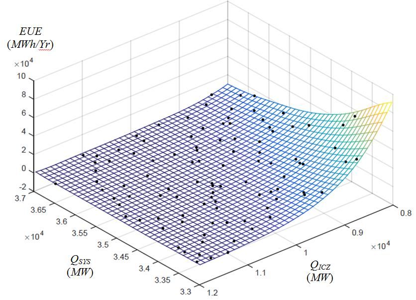
levels, i.e., EUE(QSYS, QICZ, QECZ). The multivariate surface with one ICZ and no ECZ is illustrated in Fig. 2 where the dots on
the surface represent EUEs corresponding to the sampled system and ICZ capacity levels.
3
The example can be easily extended to more complicated configurations.4
Fig.2. Multivariate EUE function
To measure the value of reliability, we introduce VOLL in $/MWh. Since reliability is treated as a public good, the same
VOLL shall apply to every MW of lost load, irrespective of its location. Therefore, the value of reliability, which is based on
the Cost of Unserved Energy (CUE), can be represented as:
CUE QSYS , QICZ , QECZ VOLL EUE QSYS , QICZ , QECZ (1)
B. Decomposition of EUE/CUE
The marginal value of reliability, or the derivative of CUE, represents consumers’ willingness to pay for reliability, or, the
demand curve. Since CUE is a multi-variate function, its derivatives, are also multi-variate functions. Multi-variate demand
functions imply coupling among capacity levels of different zones, i.e., one zone’s willingness to pay would not only depend on
the demand level of that zone, but demand levels of all other zones as well. Evaluation of the multi-variate CUE function based
on the multi-area reliability theory is much more complex than the single area reliability [23]-[26]. Furthermore, the coupling
among different capacity zones makes the demand functions difficult to interpret, and poses significant challenges to numerical
approximation of the demand functions and the market clearing process.
To address the above challenges, our approach is to decompose the EUE function (and hence CUE) into single-variable
components such that each would lead to a demand curve relating only to the capacity level of a particular zone. Approximation
may need to be involved in the decomposition as shown later in this subsection. Also, there exists multiple ways of
decomposition. The key challenge is to find an appropriate decomposition formula that yields meaningful and easy-to-interpret
demand curves. Below is our decomposition.
Loss of load can be caused either by the inadequate system capacity or the insufficient transfer capability between zones.
Therefore, a natural way of decomposing the multi-variate EUE function is to separate the two causes, i.e.,
EUE QSYS , QICZ , QECZ EUESYS QSYS EUE A|SYS QICZ , QECZ | QSYS (2)
where EUESYS(QSYS) is the expected unserved energy resulting from the system capacity deficiency (i.e., treating the entire system
as a single zone without considering zonal interface limits); and EUEA|SYS (QICZ, QECZ |QSYS) is the “additional” expected
unserved energy resulting from the distribution of system capacity QSYS in the presence of interface constraints. It can be seen
that EUESYS() is a single-variable function since it only depends on the total system capacity. However, EUEA|SYS () is still a
multivariate function as it depends on the total system capacity and its distribution in ICZ and ECZ. Further decomposition of
EUEA|SYS () is needed.
In practice, the fixed zonal capacity requirements are calculated one zone at a time [27], i.e., one zone’s capacity requirement
is not affected by other zones’ capacity allocation. The underlying assumption is that the reliability impact of one zone’s capacity
is independent of other zones’. Under the same assumption, the EUEA|SYS resulting from the distribution of system capacity can
be decomposed into individual zones, i.e.,5
EUEA|SYS QICZ , QECZ | QSYS EUEICZ |SYS QICZ | QSYS EUEECZ |SYS QECZ | QSYS (3)
where EUEICZ|SYS (QICZ |QSYS) is the additional expected unserved energy caused by the ICZ import limit when allocating QICZ of
system capacity QSYS into the ICZ; and EUEECZ|SYS (QECZ |QSYS) is the additional expected unserved energy caused by the ECZ
export limit when allocating QECZ of system capacity QSYS into the ECZ. Note that EUEICZ|SYS() and EUEECZ|SYS() depend not
only on the capacity in the corresponding zone, but the total system capacity as well. Therefore, these two functions are still
multi-variate. However, in our testing of the NE system, we found that these EUE values are not sensitive to the system capacity
QSYS around the nominal system capacity level of ICR, which corresponds to the desired “1-in-10” LOLE criterion. As a result,
EUEICZ|SYS() and EUEECZ|SYS() in (3) are approximated as
EUEICZ |SYS QICZ | QSYS EUEICZ |SYS QICZ | ICR (4)
EUEECZ |SYS QECZ | QSYS EUEECZ |SYS QECZ | ICR (5)
Ideally, the system capacity QSYS in the above approximations should be the optimal level of the system capacity from the
capacity market clearing, e.g., Q*SYS, instead of ICR. Therefore the approximation error can be measured by the difference
between EUEZ|SYS (EZ|Q*SYS) and EUEZ|SYS (EZ|ICR) where Z= ICZ or ECZ. In the lack of knowing Q*SYS prior to the market
clearing, we can specify a range [Qmin, Qmax] surrounding ICR for estimating Q*SYS, with Qmin and Qmax denoting the bounds for
possible cleared system capacity4. Then the approximation error in (4)-(5) can be capped by the deviation from EUEZ|SYS
(EZ|ICR) to EUEZ|SYS (EZ|Qmin) or EUEZ|SYS (EZ|Qmax). Our testing of the NE system found the error to be quite small.
Substituting (3)-(5) into (2), we have:
EUE QSYS , QICZ , QECZ EUESYS QSYS EUEICZ |SYS QICZ | ICR EUEECZ |SYS QECZ | ICR (6)
The right-hand side components in (6) are single-variable functions with respect to the system total capacity QSYS, ICZ capacity
QICZ and ECZ capacity QECZ, respectively. Consequently, the value of reliability, or the Cost of Unserved Energy (CUE) in (1),
can be decomposed as:
CUE QSYS , QICZ , QECZ VOLL EUESYS QSYS
(7)
VOLL EUEICZ |SYS QICZ | ICR VOLL EUEECZ |SYS QECZ | ICR
where the right-hand-side components represent the CUE associated with QSYS, QICZ and QECZ, respectively.
System reliability improves (i.e., less unserved load) when there is more capacity in the system. Therefore, EUESYS() in (6) is
a monotonically decreasing function of QSYS. Also, the capacity in ICZ has more value than that of the rest of system due to the
zone’s import limit. Therefore, system reliability improves when more capacity is allocated in ICZ, i.e., EUEICZ|SYS() in (6) is a
monotonically decreasing function of QICZ. On the other hand, system reliability deteriorates when more capacity is allocated in
ECZ where the capacity is constrained by the export limit. Namely, EUEECZ|SYS() in (6) is a monotonically increasing function of
QECZ.
C. Capacity demand curves
With the above decomposition of the value of reliability in (7), demand curve, as the marginal value of reliability for
corresponding system or zonal capacity, can be represented by the negative derivative of the corresponding CUE components in
(7) (with the negative sign to convert cost into value), i.e.,
dEUESYS QSYS
DSYS QSYS VOLL (8)
dQSYS
dEUEICZ |SYS QICZ | ICR
DICZ QICZ VOLL (9)
dQICZ
dEUEECZ |SYS QECZ | ICR
DECZ QECZ VOLL (10)
dQECZ
where DSYS(), DICZ() and DECZ(), respectively, are the system and zonal demand curves representing the annualized marginal
value of capacity in $/mw-year.
4
As we design the VOLL parameter to achieve the “1-in-10” criterion under the long-term market equilibrium (discussed in Section II.F), the optimal
system capacity Q*SYS is considered to converge to the ICR in the long run. Under the convergence, the range is bounded and would be narrower along the
convergence path, implying smaller approximation error in (4)-(5).6
The EUE components associated with system and ICZ capacities in (6) are monotonically decreasing functions. As a result,
their derivatives are negative, and the corresponding system and ICZ demand curves in (8)-(9) have positive values.
Furthermore, as we will derive in the next Section, the derivative of EUE (with the negative sign) is in general proportional to the
Loss of Load Hours (LOLH)5. The LOLH, as a reliability index, decreases when the capacity increases. Therefore the system
and ICZ demand curves are monotonically decreasing. Likewise, the ECZ demand curve in (10) has negative values and is
monotonically decreasing.
It should be noted that zonal demand curves are derived from the EUE components that reflect the additional unserved energy
caused by the interface limits. Therefore, zonal demand curves reflect the load’s additional willingness to pay for capacity in the
corresponding zones besides the marginal value of the total system capacity. The total willingness to pay for capacity in an ICZ
or ECZ zone is then a combination of the system and zonal demand curve values, i.e.,
DSYS QSYS DZ QZ , Z ICZ or ECZ . (11)
Note that the above total willingness to pay in (11) depends on both the system capacity QSYS and its allocation QZ in the zone.
With the demand curves (8)-(10), the CUE in (7) can be represented as
CUE QSYS , QICZ , QECZ 0 sys Dsys Q dQ 0 ICZ DICZ Q dQ 0 ECZ DECZ Q dQ
Q Q Q
(12)
D. Social-surplus maximization
The objective of the Forward Capacity Market (FCM) is to maximize the total surplus of capacity supply and demand, or
equivalently, to minimize the total costs of capacity offers and CUE, i.e.,
Minimize
{qi }, QSYS ,QICZ ,QECZ
Ci qi
iZ ICZ
jZ ECZ
Cj qj
kZ ROS
Ck qk
(13)
0 SYS DSYS Q dQ 0 ICZ DICZ Q dQ 0 ECZ DECZ Q dQ
Q Q Q
where ZICZ, ZECZ and ZROS, respectively, are the sets of capacity offers in ICZ, ECZ and ROS; qi, qj, and qk are the cleared
quantities of capacity offers in the corresponding zones; QICZ, QECZ and QROS are cleared demand in corresponding zones; and
Ci(·), Cj(·), and Ck(·) are the costs associated with corresponding capacity offers.
The total cleared system capacity should meet the total system demand, i.e.,
qi qj qk QSYS (14)
iZ ICZ jZ ECZ kZ ROS
Similarly, the cleared capacity in ICZ should meet the ICZ demand, i.e.,
qi QICZ (15)
iZ ICZ
For the export zone, the zonal demand serves as a “limit” instead of requirement in order to limit the capacity allocated in the
interface-constrained export zone, i.e.,
q j QECZ (16)
jZ ECZ
Each capacity offer has its own constraints, e.g., capacity size. The constraints for an offer i is denoted by Ωi. Thus we have
qi i , i Z ICZ Z ECZ Z ROS (17)
The FCM clearing problem is then (13)-(17). It can be seen that with demand curves, the FCM problem allows tradeoffs
between costs and values of capacity, and tradeoffs between capacities in different zones. These features are unavailable under
the fixed capacity requirements.
E. Capacity Clearing Prices
In this subsection, we define the capacity clearing prices and link them to the demand curves based on the KKT optimality
conditions [28] of the social-surplus maximization problem (13)-(17). We denote the Lagrange multiples associated with the
capacity constraints (14)-(16) by SYS, ICZ and ECZ, respectively. The Lagrangian of the social-surplus maximization problem is
then
5
The exact relation form between EUE and LOLH depends on the reliability evaluation process that is adopted.7
L Ci qi
iZ ICZ
jZ ECZ
Cj qj
kZ ROS
Ck qk 0 SYS Dsys Q dQ 0 ICZ DICZ Q dQ 0 ECZ DECZ Q dQ
Q Q Q
SYS QSYS qi q j qk ICZ QICZ qi ECZ q j QECZ (18)
iZ ICZ jZ ECZ kZ ROS
iZ ICZ
jZ
ECZ
Suppose that the problem (13)-(17) is convex, e.g., capacity offer costs are convex functions and demand curves are
monotonically decreasing. Then the KKT optimality conditions for the problem hold and yield the following:
SYS
*
DSYS QSYS
*
(19)
ICZ
*
DICZ QICZ
*
(20)
ECZ
*
DECZ QECZ
*
(21)
where Q*SYS, Q*ICZ and Q*ECZ, respectively, are cleared demand in system and zones; and *SYS (≥0), *ICZ (≥0) and *ECZ (≥0)
respectively, are the shadow prices associated with the system and zonal capacity constraints.
The Capacity Clearing Price (CCP) for the ROS zone can be defined as the marginal value of increasing by 1MW of capacity
in ROS (or equivalently, system capacity), i.e., DSYS(Q*SYS). Based on (19), we have
CCPROS DSYS QSYS
*
SYS
*
(22)
Similarly, the capacity clearing price for the ICZ zone can be defined as the marginal value of increasing by 1 MW of capacity in
ICZ. Together with (11), we have
CCPICZ DSYS QSYS
*
DICZ QICZ
*
SYS
*
ICZ
*
(23)
For ECZ, we have
CCPECZ DSYS QSYS
*
DECZ QECZ
*
SYS
* *
ECZ (24)
Based on (23)-(24), it can be seen that shadow prices *ICZ and *ECZ can be interpreted as “congestion components” of the
corresponding capacity zone clearing prices, e.g., if the ICZ constraint (15) or the ECZ constraint (16) is not binding, then the
corresponding shadow price becomes zero, and the ICZ or ECZ clearing price would be the same as the ROS clearing price. This
interpretation is also consistent with the EUE decomposition in (6) where the zonal EUE components that lead to the
corresponding demand curves reflect the unserved energy due to interface limits. Furthermore, since the shadow prices are non-
negative, we have the following price cascading relationship:
CCPICZ CCPROS CCPECZ , (25)
which is consistent with the intuition that the capacity of an import zone is the most valuable and the capacity of an export zone
is the least valuable.
F. Implied VOLL
Power system reliability in many ways represents a classic public good [29]-[31]. Despite the market liberalization, there’s
still a lack of a mechanism for consumers to express their reliability preferences. With the centralized capacity markets, capacity
is still purchased to achieve the uniform system reliability criterion (e.g., 1-in-10) enforced by regulatory institutions such as
North America Electric Reliability Corporation (NERC). Consequently, we consider the uniform VOLL for the entire system in
the centralized capacity market, i.e., the same value of reliability is considered for all consumers throughout the electric network.
Estimating VOLL is notoriously difficult and a wide range of values from several thousand to tens of thousands of U.S. dollars
per MWh have been reported [16]-[19]. The popular estimation methods include customer survey [32], macroeconomic analysis
[33], and case study [34]. Each of them has strengths and weaknesses. In this paper, we imply the VOLL value from Net Cost of
New Entry (Net-CONE) based on the long-term equilibrium property of the economic framework established in the previous
subsections.
Many capacity markets use the Net-CONE for market power mitigation and administrative price setting. The Net-CONE
value, calculated as the annualized capital costs for the new resource, less its expected margin from energy and reserve markets,
essentially reflects the “missing-money” or the marginal cost of the new resource. Depending on the assumptions made for the8
new resource, different markets may have different Net-CONE values. ISO-NE calculated the Net-CONE value of $11.64/kw-
month for the capacity commitment period of 2019-2020 [35]. PJM used a Net-CONE value of $102,315/MW-year for the same
period of 2019-2020 [36]. Nevertheless, the Net-CONE value is calculated prior to the FCM clearing, and we therefore can use it
to derive the implied VOLL in the following.
Based on (22)-(24) and the marginal cost meaning of Net-CONE, we have the following relations between the demand curves
and Net-CONEs:
D Q*
SYS SYS
Net _ CONESYS
DSYS QSYS DICZ QICZ Net _ CONEICZ
* *
(26)
DSYS QSYS
*
DICZ QECZ
*
Net _ CONEECZ
The above (26) represents the well-known result in microeconomics theory that the marginal benefit of demand equals the
marginal cost of new entry at the market equilibrium. Substituting (8)-(10) into (26) and denoting the negative derivative of EUE
as Marginal EUE (MEUE), we have
MEUE
SYS QSYS Net _ CONESYS VOLL
*
MEUESYS QSYS MEUEICZ |SYS QICZ | ICR Net _ CONEICZ VOLL
* *
(27)
MEUESYS QSYS *
MEUEECZ |SYS QECZ *
| ICR Net _ CONEECZ VOLL
With (27), one can calculate MEUESYS, MEUEICZ|SYS and MEUEECZ|SYS for a given VOLL. As shown in the later Section III, the
MEUE functions are monotonically decreasing and can be numerically evaluated with existing reliability assessment tools.
Therefore, one can look up the MEUE curves to obtain the system capacity and its distribution with respect to the given VOLL,
i.e., Q*SYS(VOLL), Q*ICZ(VOLL) and Q*ECZ(VOLL). With the monotonically decreasing MEUE functions and (27), Q*SYS, Q*ICZ
and Q*ECZ are monotonically increasing with respect to VOLL. This is intuitive since a higher evaluation of reliability, i.e., higher
VOLL, would lead to more installed capacity and higher reliability level.
Furthermore, with the LOLE of 0.1 days/year as the reliability criterion, it should be achieved at the market equilibrium.
Similar to EUE, the system LOLE is affected by both the total system capacity and its allocation among zones, i.e., LOLE(Q*SYS,
Q*ICZ, Q*ECZ). The existing reliability assessment software can calculate the LOLE for a given set of capacities (Q*SYS, Q*ICZ,
Q*ECZ) associated with a multi-zone model. As a result, for a given VOLL, one can first calculate the capacities based on (27) and
then run the reliability assessment software to obtain the corresponding LOLE(Q*SYS(VOLL), Q*ICZ(VOLL), Q*ECZ(VOLL)).
LOLE is monotonically decreasing when Qsys, QICZ or QECZ increases. This is obvious since adding capacity anywhere in the
system could only improve, not worsen, the system reliability. Combined with the fact that Q*SYS, Q*ICZ and Q*ECZ are
monotonically increasing functions of VOLL, the compound function LOLE is monotonically decreasing with respect to VOLL.
Based on this monotonicity property, we can obtain the VOLL value that leads to the system LOLE of 0.1 days/year by a simple
bisection algorithm.
In the case that a uniform Net-CONE is used across the system, implying no limiting interfaces at the equilibrium, the
calculation of VOLL diminishes to the following simple equation:
Net _ CONESYS
VOLL (28)
dEUESYS QSYS dQSYS QSYS ICR
Note that the above VOLL is endogenously calculated through the proposed framework, in contrast to most other demand curve
designs (e.g., [13]) that treat the VOLL as an exogenous parameter.
G. Extension of the Framework
The economic framework presented in this section is based on the ISO-NE’s capacity market that models import, export and
ROP zones. Some capacity markets, e.g., NYISO, do not model export zones but have nested import zones, e.g., one import zone
is enclosed in another import zone. The proposed method can be adapted to the nested zones by treating the outer import zone as
a subsystem and further decomposing the subsystem reliability function into the components associated with the inner import
zone and the rest of the subsystem. Also, some markets may need demand curves for inter-zonal transfer capability instead of the
zone’s capacity. Then the multi-variate reliability function, also a function of the transfer capability, will be decomposed into
components that include one single-variable function for the transfer capability. In essence, the decomposition of the reliability9
function relies on the configuration of the capacity market model, and different decompositions may involve different
approximations to the multi-variate reliability function. As a result, the applicability of the proposed method will be determined
by how good the approximation is.
The VOLL as the important scaling factor for the proposed demand curves is implied based on the 1-in-10 criterion. Different
ISOs may have different reliability criteria. Similar derivation using equilibrium conditions and the Net-CONE can be used to
imply the VOLL parameter.
III. CALCULATING DEMAND CURVES
In this section, we present a practical process of producing capacity demand curves based on the proposed theoretical
framework. EUEs and their derivatives are evaluated at different capacity levels by existing reliability assessment tools. The
implied VOLL value is also calculated. With VOLL as a scalar factor, demand curves are produced based on linear interpolation
of the EUE derivative points.
A. Reliability Evaluation
The EUEs serve as the fundamental reliability measure for deriving capacity demand curves (8)-(10). Existing reliability
assessment tools such as GE’s Multi-Area Reliability Simulation (MARS) can evaluate various reliability indices, including
EUE, LOLH and LOLE, for a multi-area system by chronological simulation of the system [37]. Details of the generator outage,
maintenance schedule, renewable resource treatment, and tie-benefit assumptions can be modeled in the reliability assessment
tool, following the ISO’s reliability assessment procedure. To produce capacity demand curves for the system and zones, the
corresponding EUE components in (6) are evaluated separately as described below.
To evaluate the EUESYS component in (6), i.e., the unserved energy resulting from the system capacity deficiency, the entire
system is modeled as one area. One can predetermine the range of system capacity levels to be evaluated, and pick the capacity
level points within the range for evaluation. The range should be chosen to cover the possible cleared system capacity level and
the number of points should be sufficient enough to characterize the shape of the demand curve. For a given system capacity
level, the reliability assessment software calculates the reliability indices through simulations. The evaluation process for each
capacity level is independent of the evaluations of other capacity levels. Therefore, the evaluation for different system capacity
levels can be carried out in parallel to improve the computational efficiency.
To evaluate zonal EUE components in (6), i.e., the additional unserved energy resulting from allocating certain capacity out
of the system ICR into the corresponding zone, the system is modeled as two areas: the ICZ or ECZ zone under consideration;
and the rest of the system. Note that zonal EUE components are considered independent of each other as described in Section II.
Therefore, the evaluation for each ICZ or ECZ is independent of each other and can be performed in parallel. For each ICZ or
ECZ zone, we select a range of capacity levels in that zone and sufficient number of sample points within the range. For each
selected capacity level, e.g., QZ (Z=ICZ or ECZ), we evaluate the reliability indices by performing the 2-area simulations with
the total system capacity held at ICR and the zonal interface limit imposed. The resulting reliability measure reflects the
reliability impact of both system capacity at ICR and its allocation of QZ in the zone. Denote the EUE measure of the 2-area
system by EUE2(Q*SYS, QZ) where Q*SYS = ICR. Then the zonal EUE component in (6) is obtained as
EUEZ |SYS QZ | ICR EUE2 ICR, QZ EUESYS ICR (29)
where EUESYS(ICR) is a constant and can be calculated during the evaluation of system EUE component. The evaluation of
different zonal capacity levels can be carried out in parallel to improve the computational efficiency.
The above description applies also to other reliability indices such as LOLH; and the reliability assessment software produces
all reliability indices simultaneously. Thus the LOLH components can be obtained along with the EUE components.
B. EUE derivatives
Capacity demand curves (8)-(10) are the derivatives of EUE components. With EUE components for various capacity levels
obtained from subsection III.A, a simple numerical approximation6 of the EUE derivative at each capacity level is the average
slope of the two linear segments adjacent to the capacity point as illustrated in Fig. 3.
6
More sophisticated numerical approximations are out of the scope of this paper.10
EUE
EUEi-1 Slopei
i
EUE Slopei+1
i+1
EUE
Q
Qi-1 Qi Qi+1
Fig.3. Approximate EUE derivative.
The EUE derivative at capacity level Qi is then calculated as:
dEUE Q
EUE EUE
i i 1
EUE i 1 EUE i
/ 2 (30)
i 1 i 1
dQ Q Qi
Q i
Q Q Q i
Alternatively, the EUE derivatives can be obtained from the LOLH values, thus avoiding the numerical approximation of EUE
derivatives. This is achieved by using the relationship between EUE derivative and LOLH as demonstrated below.
Each EUE component (system or zonal) in (6) is a single-variable function of the corresponding capacity Q. The EUE(Q) is
basically the average hourly Loss of Load (LOL) across simulated years, i.e.,
N
EUE Q LOLn,h Q N (31)
n 1 h
where n and h, respectively, are the indices of the simulated years and hours, N is the total number of the simulated years, and
LOLn,h(Q) is the loss of load in MWs for Hour h of Year n under Q. Now consider a small firm load change dL. The change of
EUE caused by dL can be represented as
N
dEUE Q dL I LOLn,h Q 0 N (32)
n1 h
where I LOLn,h Q 0 is the indicator variable indicating non-zero LOL. Based on the definition of LOLH, i.e.,
N
LOLH Q I LOLn,h Q 0 N, (33)
n 1 h
we have
dEUE Q dL LOLH Q (34)
The firm load change can be translated to the capacity change. For instance, one can convert dQ to dL by the average Equivalent
Forced Outage Rate – in Demand (EFORd), i.e.,
dL dQ 1 EFORd . (35)
From (35)-(36), we have
dEUE dQ LOLH Q 1 EFORd . (36)
C. Producing demand curves
With the derivatives of EUE components for selected capacity levels calculated in Subsection III.B, we create continuous
demand curves based on these evaluated capacity levels. Demand curves should be monotonically decreasing. Due to the
statistical nature of reliability simulation and the possible numerical approximation error introduced by (30), the calculated EUE
derivative values at the selected capacity levels may not be monotonic. Therefore, we first ensure monotonicity of the points. A
simple filter that checks all points and removes the non-monotonic ones can be applied. These points can be simply connected to
form a piece-wise linear curve. Then the system EUE derivative that corresponds to ICR7 can be found to calculate the VOLL
based on (28). The piece-wise linear curve of EUE derivatives is then scaled with VOLL to produce the corresponding system or
7
The system Installed Capacity Requirement (ICR) is the capacity level where the 1-in-10 LOLE is met, i.e., LOLE(ICR) =0.1. ICR can be obtained by
linear search since LOLE(Q) is a monotonically decreasing function of Q.11
zonal capacity demand curve based on (8)-(10). The above process to generate demand curves is summarized in the diagram
below.
Select Capacity Range and Calculate EUE
Sample Points for Derivatives for Selected
Reliability Evaluation Capacity Points
Evaluate System
Estimate VOLL
Reliability for Selected
Capacity Points
Produce Demand
Curves with VOLL and
EUE Derivatives
Fig.4. Demand curve process
IV. CASE STUDY
In this section, we first present a 2-zone analytical example to demonstrate the demand curve derivation and the FCM
clearing. Then, we apply the process in Section III to a multi-zone ISO-NE system, and analyze the resulting demand curves.
Case 1. Analytical Example
Consider a 2-zone system with one ICZ and the ROS. Assume that the multivariate EUE function has an analytical form of
EUE(QSYS, QICZ) = 106/QSYS + 8000/QICZ. The Net-CONE value is $10/kw-month. The block capacity offers in ICZ and ROS are
summarized in Table 1.
Table 1. Capacity offers
Zone Block 1 Block 2 Block 3
Capacity (MW) 200 150 150
ROS
Price ($/kw-month) $6 $9 $10.5
Capacity (MW) 300 200 200
ICZ
Price ($/kw-month) $5 $8 $10
Since the assumed multivariate EUE function is separable in QSYS and QICZ (an assumption used for the simplicity of analysis and
does not hold for actual systems), the EUE components for the system and ICZ are naturally obtained as
EUESYS QSYS 106 QSYS and EUEICZ |SYS QICZ 8000 QICZ (37)
Note that the zonal EUE component EUEICZ|SYS does not rely on the system capacity QSYS due to the above assumption. The
derivatives of the corresponding EUE components, respectively, are:
dEUESYS QSYS dQSYS 106 QSYS
2
and dEUEICZ |SYS QICZ dQICZ 8000 QICZ
2
(38)
As analyzed in Section III.2, the derivative of EUE has certain relations to the corresponding LOLH, depending on how firm
load is translated into the installed capacity. For the simplicity of analysis, we assume that LOLH is the negative EUE derivative,
i.e.,
LOLH SYS QSYS 106 QSYS
2
and LOLH ICZ |SYS QICZ 8000 QICZ
2
(39)
Furthermore, we assume that 1 hour of LOLH translates into 0.1 day of LOLE. Then,
LOLESYS QSYS 105 QSYS
2
and LOLEICZ |SYS QICZ 800 QICZ
2
(40)
Based on the system LOLE function in (40), one can calculate the ICR that corresponds to 0.1 day/year LOLE, i.e., ICR
=(105/0.1)0.5=1000 MW. Then based on (38), the system EUE derivative at the ICR is calculated as dEUESYS/dQSYS = 1.
Therefore the VOLL is calculated with (28), i.e.,12
VOLL 10 / (1) $10 / kw month $120,000 / mwh (41)
The system and zonal demand curves are derived from the EUE derivatives in (38) scaled by the VOLL, i.e.,
DSYS QSYS 107 QSYS
2
and DICZ QICZ 8 104 QICZ
2
(42)
These curves are illustrated in Fig. 5.
Fig.5. Demand curves for the 2-zone example
With the demand curves in (42) and the capacity offers in Table 1, the FCM clearing problem (13)-(17) can be solved and yield
the following solution:
Table 2. Clearing result for the 2-zone example
Cleared Capacity Cleared Demand Clearing Price
q* (MW) Q* (MW) ($/kw-month)
ICZ 600 600 10.5
ROS 400 1000 (Q*SYS) 10
In the following, we interpret the above clearing result based on the meaning of demand curves.
As discussed in Section II.3, the load’s willingness to pay for capacity in ICZ, or the incremental reliability value in ICZ, is
reflected by the combination of system and zonal demand curve values. At the system capacity Q*SYS = 1000MW, the system
demand value is $10/kw-month. Therefore, the total willingness to pay in ICZ can be viewed as the zonal demand curve in Fig.5
shifted upward by $10. The clearing of the ICZ can then be illustrated by the intersection of the raised demand curve and the
aggregated supply offer curve in ICZ (see Fig. 6). It can be seen that the two curves intersect at q*ICZ = Q*ICZ = 400MW and
$10.5/kw-month. These are consistent with the cleared quantity and clearing price in Table 2.
Next we consider the entire system. According to Section II.3, the load’s willingness to pay for the system capacity (absent
zonal interface limits) is reflected by the system demand curve in Fig.5. The system supply curve should combine both the
capacity offers in ROS and ICZ. With the cleared 400MW in ICZ, the system supply curve is the aggregated supply offer curve
in ROS shifted to the right by 400MW. The clearing of the system can then be illustrated by the intersection of the shifted supply
curve and the system demand curve (see Fig. 6). It can be seen that the two curves intersect at q*SYS = Q*SYS = 1000MW
(including the 400MW cleared ICZ capacity) and $10/kw-month. These are consistent with the cleared quantity and clearing
price in Table 2.
Fig.6. FCM clearing for the 2-zone example13
Case 2. ISO-NE System
ISO-NE’s 11th FCM for the 2020-2021 commitment period is used for the study. The auction base cases including network
configuration can be found in [38]. The system has 1 import zone (SENE), 1 export zone (NNE), and the Rest of System zone.
GE-MARS is used for reliability simulations, which were run on Amazon Cloud. All the numerical results can be found in [39].
System demand curve
The system EUE component EUESYS is evaluated on sample capacity levels within the range of [32.02GW, 37.44GW] at
10MW sample interval. To derive the system demand curve, we took the numerical approximation8 of EUESYS at the sampled
capacity levels. The EUE derivatives at these capacity levels are depicted in Fig. 7.
Fig.7. System EUE component and derivative.
It can be seen that the EUE derivative is monotonically decreasing. Since EUE derivative reflects LOLH, a reliability index, this
can be explained by the fact that reliability improves when more capacity is added into the system.
The system ICR that corresponds to 1-in-10 LOLE has been calculated by the ISO at 34,070 MW [39]. Based on the EUE
derivatives in Fig.7, we obtain the derivative of EUESYS at the ICR as -0.6465 hours/year. Also, NET_CONE for the FCM has
been predetermined by the ISO at $11.64/kw-month. Therefore, VOLL can be determined as follows based on (29):
VOLL 11.64 / 0.6465 12000 $216,048 / MWh (43)
The above VOLL implied from NET-CONE can be compared to the values obtained through other methods such as customer
survey, which opens the door for research on different VOLL estimation methods. The system demand curve is obtained as the
linear interpolation of EUESYS points scaled by VOLL and is shown in Fig. 8.
Fig.8. System demand curve.
Zonal demand curves
Zonal demand curves are derived from the derivatives of the corresponding zonal EUE components. Based on (36), we use
LOLH for zonal demand curves to avoid numerical approximation of EUE derivative. Zonal LOLH values are functions of the
corresponding zonal capacity levels. We evaluate LOLH for selected zonal capacity levels within the selected range for each
zone individually while holding the system capacity at ICR. The zonal demand curves are obtained as the linear interpolation of
the LOLH points scaled by the VOLL. These zonal demand curves are depicted in Fig.9.
8
Note that the EUE derivative can also be obtained through LOLH as mentioned in Section III. However, for the system EUE, the relationship between
LOLH and EUE derivative is more complex than (36) due to the specific reliability evaluation procedure. Therefore, we adopt the numerical approximation for
the system EUE derivative.14
Fig.9. Demand curves for the import SENE and export NNE zones.
It can be seen that the SENE (import zone) demand curve approaches zero when the capacity allocated in the zone increases, and
the NNE (export zone) demand curve starts with zero where the capacity allocated in the zone is small. This is because the
interface tends not to be constrained when more capacity is allocated in the import zone or less capacity is allocated in the export
zone. This is consistent with our analysis in Section II that the zonal demand curves act as congestion components in FCM
pricing.
V. CONCLUSION
This paper presents an economic framework for deriving demand curves in Forward Capacity Markets (FCM). Unlike the ad
hoc demand curves implemented in the existing capacity markets, our approach is built on a rigorous economic and mathematical
foundation. Also, an innovative decomposition of EUE is developed to obtain the single-variable demand curves. The resulting
demand curves have a clear economic meaning that reflects the reliability impact of capacity in corresponding zones. Our
approach may also be used to derive demand curves for other products such as reserves, and the result of our approach has
broader impacts on other interesting research topics such as VOLL estimation.
REFERENCES
[1] P. Joskow and J. Tirole, “Reliability and Competitive Electricity Markets,” The RAND Journal of Economics, Vol. 38, No. 1, pp. 60-84, March 2007
[2] D. Newbery, “Missing money and missing markets: Reliability, Capacity Auctions and Interconnectors,” Cambridge Working Paper in Economics,
no.1513, Jul. 2015
[3] P. Cramton, A. Ockenfels and S. Stoft, “Capacity market fundamentals,” Economics of Energy & Environmental Policy, Vol. 2, No.2, 2013
[4] H. Chao, “Peak load pricing and capacity planning with demand and supply uncertainty,” The Bell Journal of Economics, Vol. 14, No. 1, 1983
[5] R. Cohen, “Capacity Mechanisms in Europe: If there is to be a capacity mechanism, then what is the appropriate design”, European Commission, Sep.
2015. [Online]. Available: http://ec.europa.eu/competition/sectors/energy/slides_cohen_en.pdf
[6] FERC, Centralized Capacity Market Design Elements (Commission Staff Report AD13-7-000), [Online]. Available:
https://www.ferc.gov/CalendarFiles/20130826142258-Staff Paper.pdf
[7] PJM, VRR Curve Report, [Available] http://www.pjm.com/~/media /documents/reports/20140515-brattle-2014-pjm-vrr-curve-report.ashx
[8] NYISO, Installed Capacity (ICAP) market, [Available]
http://www.nyiso.com/public/webdocs/markets_operations/services/market_training/workshops_courses/Training_Course_Materials/NYMOC_MT_ALL
_201/Installed_Capacity.pdf
[9] MISO, Issues Statement on Facilitating Resource Adequacy in the MISO Region, [Online].Available: https://www.misoenergy.org/Library
[10] C. Hamal and J. Murphy, “Toward a capacity demand curve market” (LECG), [Online]. Available: http://mthink.com/legacy
/www.utilitiesproject.com/content/pdf/utp5_wp_hamal.pdf
[11] S. Benedettini, “PJM and ISO-NE forward capacity markets: a critical assessment” (Research Report), Centre for Research on Energy and Environmental
Economics and Policy, ISSN 2036-1785, no.12, July 2013.
[12] B. F. Hobbs, J. G. Inon, M. Hu, S. E. Stoft and M. Bhavaraju, “A Dynamic Analysis of a Demand Curve-Based Capacity market proposal: The PJM
Reliability Pricing Model,” IEEE Transactions on Power Systems, Vol. 22, No. 1, pp. 3-14, Feb. 2007
[13] W. W. Hogan, "A model for a zonal operating reserve demand curve," Oct. 2009. [Online]. Available: http://www.ksg.harvard.edu/fs/whogan/
[14] The Brattle Group, “2014 PJM Variable Resource Requirement Parameter Review,” 2014. [Online]. Available: www.pjm.com
[15] A. M. Rudkevich, “Economically justified locational criteria of the security of supply,” 9th International Conference on the European Energy Market, pp.
1-9. May 2012
[16] M. Rios, D. Bell, D. Kirschen, et. al, “Computation of the value of security,” Final Report, Oct. 1999, [Online] www2.ee.washington.edu
[17] Reliability Panel, “Review of the value of lost load report,” National Electricity Code Administrator, Jun. 2003, [Online]. Available:
http://www.neca.com.au/Files/RP_VOLL_issues_paper_report_Dec2003.pdf
[18] SEM Committee, “The value of lost load, the market price cap and the market price floor,” (Consultation Paper), AIP-SEM-07-381, 2007
[19] “Estimating value of lost load” (Report), London Economics, 2013, [Online] Available: www.ofgem.gov.uk/publications-library
[20] F. Zhao and E. Litvinov, “Defining and pricing capacity product in capacity markets,” IEEE PES General Meeting, Jul. 2010
[21] R. Billinton and R. N. Allan, “Reliability evaluation of engineering systems: concepts and techniques,” Springer, 2nd Edition, 1992
[22] A. P. Sanghvi, N. J. Balu, and M. G. Lauby, "Power system reliability planning practices in north America," IEEE Trans. Power Systems, vol. 6, no. 4,
pp. 1485-1492, Nov. 1991.
[23] C. Singh, Z. Deng, “A new algorithm for multi-area reliability evaluation - simultaneous decomposition-simulation approach,” Electric Power System
Research, Vol. 21, No. 2, pp. 129-136, Jun. 1991.
[24] T. C. Justino, C. L. Tancredo Borges, A. C.G. de Melo, "Multi-area reliability evaluation including frequency and duration indices with multiple time
varying load curves," International Journal of Electrical Power & Energy Systems, Vol. 42, No. 1, pp. 276–284, Nov, 2012
[25] G. C. Oliveirra, S. H. F. Cunha, M.V.F. Pereira, "A Direct Method for Multi-Area Reliability Evaluation," IEEE Transactions on Power Systems, Vol.2,
No. 4, pp. 934-940, Nov. 1987
[26] R. Nagarajan, C. Singh, "Multi-area reliability evaluation using composite system framework," 2016 IEEE International Conference on Power System
Technology (POWERCON).
[27] ISO-NE ICR, LSR and MCL, [Online] http://www.iso-ne.com/static-
assets/documents/genrtion_resrcs/reports/nepool_oc_review/2012/icr_2015_2016_report_final.pdf15
[28] R. T. Rockafellar, Convex Analysis, Princeton University Press, December 23, 1996
[29] D. Toomey, W. Schulze, R. Schuler, R. Thomas, J. Thorp, "Reliability, Electric Power, and Public Versus Private Goods: A New Look at the Role of
Markets," Proceedings of the 38th Annual Hawaii International Conference on System Sciences (HICSS), Track 2, 2005.
[30] S. S. Oren, "Ensuring Generation Adequacy in Competitive Electricity Markets," University of California Energy Institute Policy & Economics, Paper
EPE-007, June 3, 2003.
[31] L. Kiesling and M. Giberson, “Electric Network Reliability as a Public Good,” Presentation at CMU Conference: Electricity Transmission in Deregulated
Markets: Challenges, Opportunities, and Necessary R&D Agenda, Pittsburgh, Pennsylvania, December 15-16, 2004.
[32] CRA International, Assessment of the Value of Customer Reliability (VCR). August 12, 2008. [Online]. Available: www.ea.govt.nz/dmsdocument/6961
[33] Leahy, E., and R.S.J. Tol, An estimate of the value of lost load for Ireland, Energy Policy, 39(3), pp. 1541-1520. 2011.
[34] Billington, Tollefson and Wacker, “Assessment of electric service reliability worth,” International Journal of Electrical Power & Energy Systems, 15 (2):
95-100.
[35] ISO-NE, FCM parameters, [Online]. Available: http://www.iso-ne.com/markets-operations/markets/forward-capacity-market
[36] PJM, RPM parameters, [Online]. Available: http://www.pjm.com/~/media/markets-ops/rpm/rpm-auction-info/2019-2020-rpm-bra-planning-parameters-
report.ashx
[37] GE Energy, MARS software, [Online]. Available: http://www.geenergy consulting.com /practice-area/software-products/mars
[38] ISO-NE, FCA-11 base cases, [Online]. Available: https://smd.iso-ne.com /markets-administration/ceii/fcm/2020_2021_fca_ol_v32.zip
[39] ISO-NE, FCA-11 demand curves, [Online]. Available: http://www.iso-ne.com /static-assets/documents/2016/08/PSPC08252016_FCA11_
Demand_Curves_Values.xlsx
VI. BIOGRAPHIES
Feng Zhao (M’08) received B.S. in Automatic Control from Shanghai JiaoTong University, China in 1998, M.S. in Control Theory & Control Engineering
from Tsinghua University, China in 2001, and Ph.D. in Electrical Engineering from University of Connecticut, USA in 2008. Currently he is a Principle
Analyst at ISO New England. His research interests include mathematical optimization, power system planning & operations, and economics of electricity
markets.
Tongxin Zheng (SM’08) received the B.S. degree in electrical engineering from North China Institute of Electric Power, Baoding, China, in 1993, the M.S.
degree in electrical engineering from Tsinghua University, Beijing, China, in 1996, and the Ph.D. degree in electrical engineering from Clemson University,
Clemson, SC, in 1999. Currently, he is a Technical Manager at the ISO New England. His main interests are power system optimization and electricity market
design.
Eugene Litvinov (SM’06, F’13) received the B.S. and M.S. degrees from the Technical University, Kiev, Ukraine, and the Ph.D. degree from Urals
Polytechnic Institute, Sverdlovsk, Russia. Currently, he is the Chief Technologist at the ISO New England, Holyoke, MA. His main interests include power
system market-clearing models, system security, computer applications in power systems, and information technology.You can also read