Clustering PPI data by combining FA and SHC method
←
→
Page content transcription
If your browser does not render page correctly, please read the page content below
Lei et al. BMC Genomics 2015, 16(Suppl 3):S3
http://www.biomedcentral.com/1471-2164/16/S3/S3

 PROCEEDINGS                                                                                                                                  Open Access

Clustering PPI data by combining FA and SHC
method
Xiujuan Lei1,2, Chao Ying1, Fang-Xiang Wu3*, Jin Xu2
From 10th International Symposium on Bioinformatics Research and Applications (ISBRA-14)
Zhangjiajie, China. 28-30 June 2014

  Abstract
  Clustering is one of main methods to identify functional modules from protein-protein interaction (PPI) data.
  Nevertheless traditional clustering methods may not be effective for clustering PPI data. In this paper, we proposed
  a novel method for clustering PPI data by combining firefly algorithm (FA) and synchronization-based hierarchical
  clustering (SHC) algorithm. Firstly, the PPI data are preprocessed via spectral clustering (SC) which transforms the
  high-dimensional similarity matrix into a low dimension matrix. Then the SHC algorithm is used to perform
  clustering. In SHC algorithm, hierarchical clustering is achieved by enlarging the neighborhood radius of
  synchronized objects continuously, while the hierarchical search is very difficult to find the optimal neighborhood
  radius of synchronization and the efficiency is not high. So we adopt the firefly algorithm to determine the optimal
  threshold of the neighborhood radius of synchronization automatically. The proposed algorithm is tested on the
  MIPS PPI dataset. The results show that our proposed algorithm is better than the traditional algorithms in
  precision, recall and f-measure value.

Introduction                                                                        two modules that have the highest similarity. Restricted
Protein-protein interaction(PPI) data [1] have been very                            Neighborhood Search Clustering (RNSC) algorithm [9] is
important sources in the researches of life science, which                          another kind of clustering algorithm based on graph parti-
can explore biological functions so as to deeply under-                             tioning, which starts with a random partition of a network
stand the essence of life activities and mechanism of dis-                          and iteratively moves the nodes on the border of a cluster
eases. Clustering analysis of PPI data is an effective way to                       into the adjacent cluster to search for a better clustering
predict the function modules and protein complex and,                               result with the minimum cost. Clique Percolation Method
study mechanisms, diagnosis and treatment of diseases.                              (CPM) was put forward by Palla [10], in which the k-
  PPI data are often represented as PPI network. Tradi-                             cliques was identified by using clique percolation firstly,
tional clustering methods do not perform well for PPI data                          and then the adjacent k-cliques were combined to get the
due to the properties of their represented networks such                            functional modules. Bader et al. proposed molecular com-
as small world and scale free characters [1,2]. Many new                            plex detection (MCODE) [11], in which every node was
algorithms were proposed for clustering PPI networks                                weighted by the node’s local neighbor density firstly, then
[3,4]. In 2002 years, Girvan and Newman[5] proposed a                               the nodes with high weights were picked as the seed nodes
clustering algorithm based on hierarchical divisions, which                         of initial clusters and further these clusters were augmen-
deletes the edge with the biggest betweenness [6,7] con-                            ted to form the preliminary clusters. Markov clustering
stantly to separate modules. The Newman fast algorithm                              (MCL) [12] is a graph clustering based on flow simulation,
[8] is a kind of clustering algorithm based on hierarchy                            which has been applied to detect functional modules
condensations, in which the algorithm continually merges                            through simulating random walks within a graph. Spectral
                                                                                    clustering-based (SC) method [13] converts the problem
* Correspondence: faw341@mail.usask.ca                                              to a quadratic optimization with constraints by utilizing
3
 Division of Biomedical Engineering, University of Saskatchewan, Saskatoon,         the methodology of matrix analysis, which is generally
SK S7N 5A9, Canada                                                                  applied to the fields of image segmentation and complex
Full list of author information is available at the end of the article
                                       © 2015 Lei et al.; licensee BioMed Central Ltd. This is an Open Access article distributed under the terms of the Creative Commons
                                       Attribution License (http://creativecommons.org/licenses/by/4.0), which permits unrestricted use, distribution, and reproduction in
                                       any medium, provided the original work is properly cited. The Creative Commons Public Domain Dedication waiver (http://
                                       creativecommons.org/publicdomain/zero/1.0/) applies to the data made available in this article, unless otherwise stated.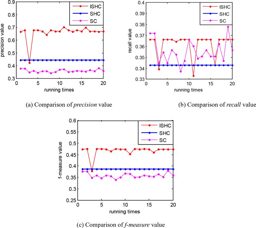
Lei et al. BMC Genomics 2015, 16(Suppl 3):S3                                                                  Page 2 of 10
http://www.biomedcentral.com/1471-2164/16/S3/S3

network clustering. Some methods advise that we should        automatic control, robot path planning and other fields.
consider the gene expression data and detect protein com-     The firefly algorithm (FA) [33-35] is an intelligent opti-
plexes basing on uncertain graph model [14,15],There are      mization algorithm developed by simulating the glowing
many new algorithms also, such as Ovrlp, PE-WCC,              characteristics of fireflies based on group searching. The
UVCluster, AP, GFA, ADMSC, SCI-BN, CORE, FAG-EC,              bionic principle of the FA algorithm is looking for part-
HC-PIN, IPCA, CP-DR, LF-PIN, ABC algorithm [16-29]            ners in the searching area according to the glowing
and so on.                                                    characteristics of fireflies, and then moving towards the
  Synchronization is a natural phenomenon ranging from        brighter firefly. Regarding points in the solution set as
the metabolism in the cell to social behavior in groups of    fireflies, the searching process in solution space is
individuals regulating a large variety of complex pro-        viewed as attraction and movements of fireflies. After
cesses. The sync [30] algorithm inherited from synchro-       many times of movements, all individuals will be gath-
nization, which is a novel approach to cluster objects        ered in the position with the highest brightness of fire-
inspired by the powerful concept of synchronization. The      flies, so as to achieve optimization. The process of
basic idea is to regard each object as a phase oscillator     optimization of the firefly intelligent algorithm is simple
and simulate their interaction behaviors over time. The       and efficient, and therefore is widely applied to func-
similar phase oscillators synchronize together and form       tional optimization and combinatorial optimization.
distinct clusters naturally along with time increasing.          Combining the advantages of the SHC algorithm and
Without depending on any distribution assumptions, the        the optimization ability of the FA algorithm noted
sync algorithm can detect clusters of arbitrary number,       above, it is naturally to adopt the FA to improve the
shape and size. In addition, because the outliers do not      SHC algorithm. Using the FA algorithm to find the opti-
synchronize with cluster objects, the concept of synchro-     mal value of synchronous neighborhood radius will be
nization allows handling the natural outliers. However,       more efficient and accurate than the basic hierarchical
the running time of the algorithm is too long to process      search do. In addition it is applicable to arbitrary data
the large-scale data. The running time of the algorithm       distribution.
consists of two parts primarily: the dynamic interaction         The paper is organized as follows: in Section “Materials
time of synchronizing objects and the process of deter-       and method”, basic concepts and principles are intro-
mining the optimal synchronous neighborhood radius.           duced firstly; secondly the proposed model of clustering
For reducing the dynamic interaction time of synchroni-       is discussed, and then the flow chart is listed, along with
zation of data, the concept of ε-neighborhood closures        the time complexity analysis of the algorithm. Perfor-
was proposed in the synchronization-based hierarchical        mance and evaluation of the proposed algorithm is
clustering (SHC) [31,32] algorithm, the objects in a          shown by comparing with SC and SHC in Section
neighborhood closures will reach synchronization com-         “Results and Discussions”. The last Section concludes
pletely and eventually form a cluster. So it can detect       this research.
clusters by putting the objects in the same neighborhood
closures to a cluster even if the objects do not synchro-     Materials and method
nize completely. However, the SHC algorithm determines        The SHC algorithm
the optimal value of synchronous neighborhood radius by       The phenomenon of synchronization often appears in
means of hierarchical search that the sync algorithm          physics, it can be expressed as follows. Two or more
does. The hierarchical search for the optimal value of        dynamic systems both have their own evolution and
synchronous neighborhood radius not only has low effi-        mutual coupling. This effect can be either one-way or
ciency but also has other two shortcomings. The hier-         two-way streets. When meets certain conditions, the
archical search is very difficult to find the optimal value   output of these systems will eventually converge and
of synchronous neighborhood radius, and the hierarchi-        completely be equal under the influence of coupling,
cal incremental Δε needs to be adjusted according to the      this process is called synchronization. The Kuramotom
different object distributions.                               model [36,37] is applied widely as the simple model of
  Swarm intelligence optimization algorithm is a kind of      synchronization behavior, the generalized definition of
bionic algorithms developed in recent years, which is         Kuramotom model is shown as follows:
characterized by simply handling, collateral implementa-        Definition 1 (Generalize Kuramoto model): The Kura-
tion and strong robustness. The searching process for         moto model consists of a population of N coupled phase
the optimal value of swarm intelligence optimization          oscillators θi(t) whose dynamics are governed by:
does not require the solution set differentiable or even

                                                                             N
continuous. So the swarm intelligence optimization               θi = ωi +         Kij sin(θj − θi )                  (1)
algorithm is applied extensively to pattern recognition,                     j=1
Lei et al. BMC Genomics 2015, 16(Suppl 3):S3                                                                                Page 3 of 10
http://www.biomedcentral.com/1471-2164/16/S3/S3

  where ωi is its natural frequencies and is distributed
with a given probability density g(ω).
  Each oscillator tries to run independently at its own
frequency, while the coupling tends to synchronize it to
all the others.
  The sync algorithm is a novel approach for clustering
inspired by the powerful concept of synchronization. It
regards each data object as a phase oscillator, and each
dimension coordinates corresponding to a phase value of
the oscillator. Each object couples with data objects in its
ε-neighborhood, where ε is the neighborhood radius. In
the effect of synchronization coupling, the object’s coordi-
nates are transformed constantly, and objects with the
same coordinates will be classified eventually to the same                  Figure 1 ε-neighborhood closures.
cluster, namely synchronization completion. Let x ∈ Rd
represents an object in the dataset X and xi be the i-th
dimension of the object x. The transformation formula of                   of the hierarchical search that the sync algorithm does.
coordinate of x shows as follows.                                          The process of hierarchical search for the optimization
                                                                           of the neighborhood radius shows as follows. Starting in
                              1                                           a small neighborhood radius value ε, then adding an
   xi (t + 1) = xi (t) +                      sin(yi (t) − xi (t)) (2)
                         Nε (x(t)) y∈N (x(t))                            increment (marked as Δε) to ε at a time (ε = ε + Δε)
                                        ε

                                                                           until the neighborhood radius is large enough to contain
  where ε-neighborhood is defined in Definition 2                          all objects. Clustering in each neighborhood radius of ε,
below.                                                                     and it is considered to be optimal when the ε gets the
  Definition 2 (ε-neighborhood): The ε-neighborhood                        best result of clustering.
radius of an object is a collection of data with distances
to the object less than ε:                                                 The FA
                                                                       The FA is a random optimization algorithm constructed
    Nε (x) = y ∈ X|dist x, y ≤ ε                       (3)
                                                                           by simulating the group behavior of the fireflies. There
   where dist(x,y) is the metric function of distance and the              are two important elements in the FA, the light intensity
Euclidean distance is often used. If the object y ∈ Nε(x), y               and the attractiveness. The former reflects the advan-
is called the ε-neighborhood of x, denoted by x ®ε y. The                  tages and disadvantages of locations of fireflies and the
relationship of ε-neighborhood between objects is symme-                   latter determines the movement distances of fireflies
trical, namely if x ®ε y then y ®ε x.                                      attracted. The optimization process of the algorithm is
   For reducing the dynamic interaction time of synchroni-                 implemented through updating the light intensity and
zation of data in the sync algorithm, the concept of neigh-                the attractiveness constantly. The mathematical mechan-
borhood closures is proposed in SHC algorithm. Objects                     ism of the FA is described as follows.
in a ε-neighborhood closure will reach synchronization                       The relative value of the light intensity of fireflies is
complete eventually. So it can detect the clusters even if                 expressed as:
the objects have not yet reached the same coordinates by                      I = I0 × e−γ rij                                       (4)
classifying data in the same neighborhood closures to the
same cluster, which reduces the dynamic interaction time                      where I0 is the initial light intensity (r = 0) related to
of data.                                                                   the objective function value, the higher the value of
   Definition 3 (ε-neighborhood closures): Suppose objects                 objective function is, the stronger the initial light inten-
set X’ ⊆ X, in the dynamic process of synchronous cluster-                 sity I0 will be. g is the light absorption coefficient set to
ing, if ∀x, y ∈ X’ satisfies x ®ε y, and if ∀x ∈ X, x ®ε z,                reflect the features that the light intensity decreases gra-
then z ∈ X’, X’ is called an ε-neighborhood closure, that is,              dually along with the increase of the distance and the
for any object x ∈ X’, Nε(x) = X’ is established.                          absorption of the medium. It can be set to a constant.
   a1, a2, a3, a4 form a ε-neighborhood closure in the Figure 1,           rij is the space distance between firefly i and firefly j.
and will reach complete synchronization eventually.                           The attractiveness of firefly is expressed as:
   The optimal value of synchronous neighborhood
                                                                              β = β0 × e−γ rij
                                                                                                 2
                                                                                                                                     (5)
radius needs to be determined in both the sync algo-
rithm and the SHC algorithm. The SHC algorithm                               where b0 is the maximum of attractiveness. g and rij
determines synchronous neighborhood radius by means                        are the same as above.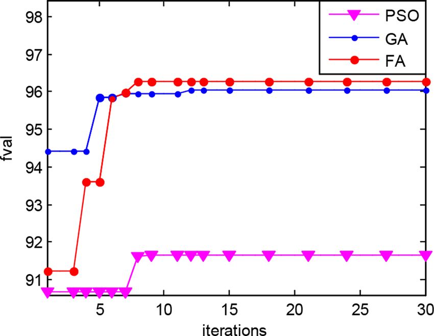
Lei et al. BMC Genomics 2015, 16(Suppl 3):S3                                                                                               Page 4 of 10
http://www.biomedcentral.com/1471-2164/16/S3/S3

   If firefly i moves to firefly j, the updating of location of     minus the average distance of all objects to its three near-
firefly i is expressed as:                                          est neighbors. So the running time of the SHC algorithm
                                                                is very huge when the dataset is uniform and dispersive. In
   xi (t + 1) = xi (t) + β × xj (t) − xi (t) + α × rand − 1/2 (6)   addition, we must set Δε small when the data distribution
                                                                    is approximate, otherwise it is hard to find the optimal
   where xi(t), xj(t) are the space coordinates of firefly i        value of synchronous neighborhood radius.
and firefly j at the time t, a is step-size in [0, 1], rand is a       The FA is a swarm intelligent optimization algorithm
random factor that follows uniform distribution in [0, 1].          developed by simulating the glowing characteristics of fire-
   Fireflies are distributed to the solution space randomly         flies, which is speedy and precise in the optimization pro-
first of all. Each firefly has its own light intensity accord-      cess. Using the firefly algorithm to search for the optimal
ing to its location, the light intensity is calculated accord-      neighborhood radius of synchronous can overcome the
ing to Eq. (4). The firefly with low light intensity is             drawbacks of the hierarchical search. It adopts fewer
attracted by and moving to the firefly with higher light            searching steps for the optimal value of synchronous
intensity. The movement distance depends on the attrac-             neighborhood radius and gets more accurate results than
tiveness between them calculated by Eq. (5). The location           the hierarchical search due to its intelligent searching stra-
updating of the fireflies is cumulated based on Eq. (6).            tegies. So it saves time on determining the optimal value
There is a disturbing term in the process of updating the           of synchronous neighborhood radius. In addition, it is
location, which enlarges the search area and avoids the             applicable to any data distributions. So we improve the
algorithm to fall into the local optimum too early. Finally         SHC algorithm by means of the FA and apply the pro-
all fireflies will gather in the location of the maximum            posed algorithm to clustering PPI data.
light intensity.                                                    Preprocessing of PPI data
                                                                    The PPI data is expressed as a graph, called PPI network,
The proposed clustering algorithm                                   in which each node represents a protein and the edge
The sync algorithm clusters objects based on the princi-            between two nodes represent the interaction between pro-
ple of dynamic synchronization, which has many advan-               teins. In that way, we get an n*n adjacency matrix of
tages in that it reflects the intrinsic structure of the            nodes. However, the dimension of the adjacency matrix is
dataset. For example, it can detect clusters of arbitrary           too big to deal with. Inspired by the spectral clustering, we
number, shape and size and not depend on any assump-                use the following way to reduce the dimension of the adja-
tion of distribution. In addition, it can handle outliers           cency matrix of PPI.
since the noise will not synchronize to cluster objects.              First, a similarity matrix A of nodes is constructed as
However, the running time of the algorithm consists of              follow.
two parts primarily: The dynamic interaction time of syn-                    ⎧
chronization of data and the process of determining the                      ⎪
                                                                             ⎨ |Ni ∩ Nj | + 1               k∈Iij w(i, k) ·    k∈I w(j, k)
                                                                               η               + (1 − η)                     ij          i = j
                                                                       Aij =     min(Ni , Nj )                      w(i, s) · t∈Ij w(j, t)          (7)
optimal value of synchronous neighborhood radius,                            ⎪
                                                                             ⎩
                                                                                                             s∈N  i
                                                                                                         0,                                i=j
which is too long to process large-scale data.
   Aiming to reduce the dynamic interaction time of the                where N i , N j are neighbor nodes of nodes u and v
sync algorithm, the concept of ε-neighborhood closures is           respectively. Iij is the common neighbors of i and j, w(i,j)
proposed in the SHC algorithm. It classifies objects in the         is the weight between i and j to measure the interaction
same neighborhood closures to a cluster even if objects             strength, and h is constant between 0 and 1.
have not yet reached the same coordinate, which enhances               Eq. (7) considers two aspects of the aggregation coeffi-
the efficiency of the algorithm by reducing the time of             cient of edges and the weighted aggregation coefficient of
dynamic interaction of data. However, the SHC algorithm             edges [38-40]. The first half of Eq. (7) is the aggregation
determines synchronous neighborhood radius by means of              coefficient of edges based on degree, which is portrayed by
hierarchical search that the sync algorithm does. The hier-         means of the ratio between adding 1 to the number of
archical search for synchronous neighborhood radius not             common neighbors of two protein nodes and minimal
only has low efficiency but also has two shortcomings.              value of the number of neighbors of two nodes. The sec-
Firstly, the hierarchical search is very difficult to find the      ond half of Eq. (7) is the weighted aggregation coefficient
optimal value of synchronous neighborhood radius in a               of edges, which is illustrated by the ratio between the pro-
fixed increment. Secondly, the increment Δε needs to be             duct of summation of weight values of edges respectively
adjusted according to different data distributions. For             connecting these two nodes (i, j) with their common
example, in the SHC algorithm, the initial value of ε is set        neighbors (k) and the product of summation of weight
to the average distance of all objects of its three nearest         values of edges linking these two nodes (i, j) with their
neighbors. The increment Δε is the different value of the           corresponding neighbors (s, t). In addition, we use h to
average distance of all objects to its four nearest neighbors       balance the weight of the two parts.
Lei et al. BMC Genomics 2015, 16(Suppl 3):S3 Page 5 of 10
http://www.biomedcentral.com/1471-2164/16/S3/S3
Then constructing Laplacian matrix L of matrix A, the Matrix X consist of the matrix L’s eigenvector that the
D is the diagonal matrix in which (i, i)-element is the top three eigenvalues corresponded. X is an n*3 matrix,
sum of A’s i-th row. in which the rows represent protein objects and the col-
⎧ umns are the three-dimensional space coordinates of
⎨ 0 Dii = 0|Djj = 0 protein objects.
Lij = Aij (8)
⎩ else
Dii Djj Step 2 The setting of parameters: the number of
firefly N, the maximum of attractiveness b0, the light
Matrix X consists of eigenvectors of matrix L’s corre- absorption coefficient g, step-size a, Maximum itera-
sponding to the first three eigenvalues and X is normal- tions maxiter, iter = 0.
ized. X is an n*3 matrix, in which lines represent the Step 3 Initialize the location of firefly in the solution
protein objects (corresponding to the protein nodes in PPI space of the neighborhood radius ε of synchronization.
network) and columns are the three-dimensional space Step 4 Do clustering respectively based on the syn-
coordinates of the protein objects. Our proposed cluster- chronous in ε that each firefly corresponding.
ing algorithm is calculated based on X. Step 4.1 Find ε-neighborhood closures of protein
Design of solution space
objects of matrix X. Objects that belong to the
The solution space of the position of the firefly corre- same closures are divided into a cluster, and then
sponds to the neighborhood radius of synchronization. mark those objects.
The initial light intensity I0 of one firefly is assigned by Step 4.2 If all points are marked, return to the
the calculation result of objective function, see Eq.(9), result of clustering, otherwise the unmarked
which is expressed as the evaluation of clustering results objects couple with the objects in its ε-neighbor-
based on the neighborhood radius of the firefly. Moving hood according to the formula (2), and then go
to the firefly with higher light intensity is regarded as to to step 4.1.
search for the optimal value of synchronous neighbor- Step 5 The light intensity of fireflies are assigned by
hood radius. The position of the firefly with the highest the calculation result of the objective function (9)
light intensity means the optimal value of synchronous according to the clustering result. Compare the
neighborhood radius. brightness of fireflies, if Ii >Ii, calculate the attrac-
Definition of objective function
tiveness according formula (5), and then update the
We choose the following object function to evaluate the location of firefly i according to the formula (6).
clustering results. Clusters with higher value of the Step 6 iter = iter+1;
objective function mean the stronger modularity of clus- Step 7 If iterLei et al. BMC Genomics 2015, 16(Suppl 3):S3 Page 6 of 10
http://www.biomedcentral.com/1471-2164/16/S3/S3
Figure 2 Flow chart of the improved SHC algorithm.
The value of r in the objective function of the FA is With practical consideration, we set the searching
important to evaluate the result of clustering. Aiming at number for the optimal threshold of the neighborhood
reflecting the correlation between fval and f-measure in radius of synchronization small values. As the value of
different r, we calculate the Pearson correlation coeffi- step-size a in FA is important to the result, we calculate
cient of fval and f-measure in 20 values that distribute 20 times to get the average value of the maximum
evenly in the region of 1 to 6 of the neighborhood objective function in different a, which is shown in
radiuses. The result is shown in Table 1 the fval and f- Table 2. Tests are carried on n = 6, maxiter = 30 cases.
measure correlation is extremely linear when r = 0.8. The average of the maximum objective function value is
Thus we set r = 0.8. optimal when a = 0.9. Thus we set step-size a = 0.9.
The Pearson correlation coefficient is shown as:
The performance comparison on different optimization
1 n Xi − X̄ Yi − Ȳ algorithms
r= (10)
n − 1 i=1 SX SY In the experiments, the dataset of PPI networks was
downloaded from MIPS database [40], which consists of
Where X̄ , Ȳ and SX, SY represent the mean value and two sets of data: one is the experimental data which
the variance of X and Y, respectively. contains 1376 protein nodes and the 6880 interactive
Table 1 Comparisons of the Pearson correlation coefficient between fval and f-measure in different r
r 0 0.1 0.2 0.3 0.4 0.5 0.6 0.7 0.8 0.9 1
r 50.9059 51.9654 52.0163 52.0588 52.0933 52.1201 52.1396 52.1521 52.1580 52.1574 52.1508Lei et al. BMC Genomics 2015, 16(Suppl 3):S3 Page 7 of 10
http://www.biomedcentral.com/1471-2164/16/S3/S3
Table 2 The average of maximum objective function values of different a for 20 times clustering (value)
a 0 0.1 0.2 0.3 0.4 0.5 0.6 0.7 0.8 0.9 1
value 94.4592 95.7940 95.4177 95.4546 95.7102 96.1161 95.2840 95.7408 95.7408 96.2709 95.7664
Table 3 The experimental parameters of PSO, GA and FA algorithms
PSO The global acceleration coefficient (c1) = 2 The local acceleration coefficient (c2) = 2
GA The crossover probability (pcro) = 0.8 The mutation probability (pmut) = 0.085
FA The maximum of attractiveness b0 = 1 The light absorption coefficient g = 1
The step-size a = 0.9
Table 4 The maximum objective function value of 10 times (value) of the FA, PSO, and GA algorithms
Algorithm 1 2 3 4 5 6 7 8 9 10
PSO 96.2709 96.2709 91.6680 96.2709 96.2709 91.6680 91.6680 96.2709 96.2709 96.2709
GA 96.2709 95.8277 95.9618 96.1602 96.0500 95.9618 95.9655 96.0500 96.2709 96.2709
FA 96.2709 96.2709 96.2709 96.2709 96.2709 96.2709 96.2709 96.2709 96.2709 96.2709
protein-pairs, which is considered the training dataset; F-measure, the harmonic mean of precision and recall is
the other describes the result that the proteins belong to defined as Eq. (13).
identical functional module, which is regarded as the
standard dataset [41], containing 89 clusters. MMS (C, F)
precison (C—F) = (11)
Inspired by the swarm optimization algorithms [42-45], |C|
we use them to search for the optimal threshold of the
neighborhood radius of synchronization. The experimental MMS (C, F)
parameters of PSO, GA and FA algorithms are shown in recall (C—F) = (12)
|F|
Table 3. The parameters of PSO and GA are set empiri-
cally based on the references [46,47]. We also calculate the
maximum objective function values for 10 times and the precision · recall
f - measure = (13)
average of the maximum objective function value over 20 precision + recall
times of the FA, the PSO, and the GA, which is shown in
Table 4 and Table 5. The plots of the optimal objective where C is the set of cluster results of training data-
function value with the number of iterations are depicted base, F stands for the set of cluster results of MIPS
in Figure 3. The FA algorithm always converges to the
optimal value fast. However, the PSO algorithm falls into a
low value sometimes, the GA algorithm gets a higher
value always. The FA performs best when considering
convergence speed and global optimization ability
comprehensive.
Precision, recall, and f-measure are employed as the
metric for clustering in this study. Precision [48] is the
ratio of the number of maximum matching nodes in train-
ing with standard database to the number of training
nodes. Recall [48] is the ratio of the largest number of
nodes in training matched the standard database to the
number of nodes in the standard database. Precision and
recall are defined as Eqs. (11)- (12), respectively while
Table 5 The average of the maximal objective function
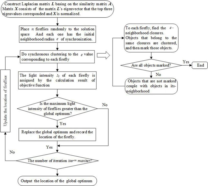
Figure 3 Plots of the optimal objective function value with the
value of PSO, GA and FA algorithms on 10 times
number of iterations of the FA, PSO and GA. (a) Comparison of
Algorithm PSO GA FA precision value (b) Comparison of recall value (c) Comparison of f-
Value 94.8900 96.0790 96.2709 measure valueLei et al. BMC Genomics 2015, 16(Suppl 3):S3 Page 8 of 10 http://www.biomedcentral.com/1471-2164/16/S3/S3 database, |C| represents the number of cluster nodes in order to obtain a more intuitive and obvious result, we training database, |F| represents the number of cluster reduce the searching number in Figure 4. We can see nodes in standard database, MMS represents the num- from the Figure 4 and Table 6 that the performance of ber of maximum matching nodes in training database the ISHC algorithm is better than the SC algorithm and with standard database. the SHC algorithm in precision, recall and f-measure. The running time of SHC algorithm and the proposed We compare our proposed algorithm with the SHC algo- algorithm are proportional to the searching number of rithm in 20 times searching as in Figure 4, the result of times, when the searching number of times is big, the our proposed algorithm is not stable sometimes. We also algorithms are impractical. So we compare the two algo- compare our proposed algorithm with some classical algo- rithms in 20 times searching. The proposed method is rithms shown in Table 6. In these algorithms we listed, compared with SC algorithm and the SHC algorithm in the result of our proposed algorithm performs best. terms of precision, recall and f-measure, respectively. The ISHC algorithm converges to the optimal thresh- Conclusion old of the neighborhood radius of synchronization stea- The sync algorithm is a novel clustering algorithm based dily when the searching number is large in Table 4. In on the model of synchronous dynamics, which can detect Figure 4 The improved algorithm compared with spectral clustering algorithm and SHC in precision, recall and f-measure.
Lei et al. BMC Genomics 2015, 16(Suppl 3):S3                                                                                                         Page 9 of 10
http://www.biomedcentral.com/1471-2164/16/S3/S3

Table 6 Comparison of precision, recall and f-measure among ISHC, SHC, SC and other algorithms
               Algorithm                                   precision                              recall                                 f-measure
               SHC[31,32]                                   0.4447                                0.3430                                   0.3873
                 SC[13]                                     0.3612                                0.3555                                   0.3584
                MCL[12]                                     0.3569                                0.3879                                   0.3717
              Newman[8]                                     0.4665                                0.4186                                   0.4413
                RNSC[9]                                     0.4067                                0.4696                                   0.4359
                  ISHC                                      0.6624                                0.3620                                   0.4673

clusters with arbitrary shape and size and has the anti-                          4.    Li M, Wang J, Chen J, Cai Z: Identifying the Overlapping Complexes in
                                                                                        Protein Interaction Networks. International Journal of Data Ming and
noise ability. However, the running time of the algorithm                               Bioinformatics 2010, 4(1):91-108.
consists of two parts primarily: The dynamic interaction                          5.    Girvn M, Newman MEJ: Community structure in social and biological
time of synchronizing data and the process of determin-                                 networks. Proceedings of the National Academy of Science 2002,
                                                                                        99(12):7821-6.
ing the optimal synchronous neighborhood radius, which                            6.    Wasserman S, Faust K: Social network analysis: methods and applications.
is too long to process large-scale data. The SHC algo-                                  Cambridge: Cambridge University Press; 1994.
rithm proposes the concept of neighborhood closures                               7.    Freeman L: A set of measure of centrality based upon betweeness.
                                                                                        Sociometry 1977, 40(1):35-41.
reducing dynamic interaction time of the sync algorithm.                          8.    Newman MEJ: Fast algorithm for dectecting community structure in
In our proposed algorithm, the efficiency and accuracy is                               networks. Physical Review E 2004, 69(6):066133.
further improved by using the FA to determine the opti-                           9.    King AD, Pržulj N, et al: Protein complex prediction via cost-based
                                                                                        clustering. Bioinformatics 2004, 20(17):3013-20.
mal thresholds of neighborhood radius of synchroniza-                             10.   Palla G, Derényi I, et al: Uncovering the overlapping community structure
tion. The recall, precision and f-measure of our proposed                               of complex networks in nature and society. Nature 2005, 435(7043):814-8.
algorithm are improved compared with SC and SHC                                   11.   Bader GD, Hogue CW: An automated method for finding molecular
                                                                                        complexes in large protein interaction networks. BMC Bioinformatics 2003,
algorithms. In future, we are intending to seek a more                                  4:article 2.
suitable model of synchronous dynamics for PPI data                               12.   van Dongen SM: Graph clustering by flow simulation. PhD thesis, Center
clustering to improve the effect of the algorithm, also the                             for Math and Computer Science (CWI) 2000.
                                                                                  13.   Ng Andrew Y, Jordan MI, Weiss Y: On spectral clustering: analysis and an
time complexity is still need to be decreased.                                          algorithm[C]. Advances in Neural Information Processing Systems Cambridge,
                                                                                        MA: MIT Press; 2001.
                                                                                  14.   Zhao B, Wang J, Li M, Wu F, Pan Y: Detecting Protein Complexes Based
Competing interests                                                                     on Uncertain Graph Model. IEEE/ACM Transactions on Computational
The authors declare that they have no competing interests.                              Biology and Bioinformatics 2014, 11(3):486-497.
                                                                                  15.   Li M, Wu X, Wang J, Pan Y: Towards the identification of protein
Declarations                                                                            complexes and functional modules by integrating PPI network and gene
The funding for the publication charges comes from: the National Natural                expression data. BMC Bioinformatics 2012, 13(1):109.
Science Foundation of China (61100164, 61173190), Scientific Research Start-      16.   Ramadan E, Osgood C, Pothen A: Discovering overlapping modules and
up Foundation for Returned Scholars, Ministry of Education of China ([2012]             bridge proteins in proteomic networks. Proc. ACM Int’l Conf. Bioinformatics
1707) and the Fundamental Research Funds for the Central Universities,                  and Computational Biology (BCB ‘10) 2010, 366-369.
Shaanxi Normal University (GK201402035, GK201302025).                             17.   Efimov D, Zaki N, Berengueres J: Detecting protein complexes from noisy
This article has been published as part of BMC Genomics Volume 16                       protein interaction data. Proc. 11th Int’l Workshop Data Mining in
Supplement 3, 2015: Selected articles from the 10th International                       Bioinformatics 2012, 1-7.
Symposium on Bioinformatics Research and Applications (ISBRA-14):                 18.   Arnau V, Mars S, Marin I: Iterative cluster analysis of protein interaction
Genomics. The full contents of the supplement are available online at http://           data. Bioinformatics 2005, 21(3):364-378.
www.biomedcentral.com/bmcgenomics/supplements/16/S3.                              19.   Frey BJ, Dueck D: Clustering by passing messages between data points.
                                                                                        Science 2007, 15(5814):972-976.
Authors’ details                                                                  20.   Feng J, Jiang R, Jiang T: A max-flow based approach to the identification
1
 School of Computer Science, Shaanxi Normal University, Xi’an, Shaanxi                  of protein complexes using protein interaction and microarray data.
710062, China. 2School of Electronics Engineering and Computer Science,                 Computational Systems Bioinformatics 2008, 7:51-62.
Peking University, Beijing,100871, China. 3Division of Biomedical Engineering,    21.   Inoue K, Li W, Kurata H: Diffusion model based spectral clustering for
University of Saskatchewan, Saskatoon, SK S7N 5A9, Canada.                              protein-protein interaction networks. PLoS ONE 2010, 5(9):e12623.
                                                                                  22.   Qi YJ, Balem F, Faloutsos C, Klein-Seetharaman J, Bar-Joseph Z: Protein
Published: 29 January 2015                                                              complex identification by supervised graph local clustering.
                                                                                        Bioinformatics 2008, 24(13):250-268.
References                                                                        23.   Leung HC, Yiu SM, Xiang Q, Chin FY: Predicting protein complexes from
1. Watts DJ, Stroqatz SH: Collective dynamics of ‘small-world’ networks.                PPI Data: A core-attachment approach. J Computational Biology 2009,
    Nature 1998, 393(6684):440-442.                                                     16(2):133-144.
2. del Sol A, O’Meara P: Small-world network approach to identify key             24.   Li M, Wang J, Chen J: A fast agglomerate algorithm for mining functional
    residues in protein-protein interaction. Proteins: Structure, Function, and         modules in protein interaction networks. International Conference on
    Bioinformatics 2005, 58(3):672-82.                                                  BioMedical Engineering and Informatics 2008, 1:3-7.
3. Wang J, Li M, Deng Y, Pan Y: Recent advances in clustering methods for         25.   Wang J, Li M, Chen J, Pan Y: A fast hierarchical clustering algorithm for
    protein interaction networks. BMC Genomics 2010, 11(Suppl 3):S10.                   functional modules discovery in protein interaction networks. IEEE
                                                                                        Transactions on Computational Biology and Bioinformatics 2011, 8(3):607-620.
Lei et al. BMC Genomics 2015, 16(Suppl 3):S3 Page 10 of 10
http://www.biomedcentral.com/1471-2164/16/S3/S3
26. Li M, Chen J, Wang J, H B, C G: Modifying the DPClus algorithm for
identifying protein complexes based on new topological structures. BMC
Bioinformatics 2008, 9:398.
27. Wang J, L B, L M, Pan Y: Identifying protein complexes from interaction
networks based on clique percolation and distance restriction. BMC
Genomics 2010, 11(Suppl 2):S10.
28. Ren J, Wang J, Li M, Wang L: Identifying protein complexes based on
density and modularity in protein-protein interaction network. BMC
Systems Biology 2013, 7:S12.
29. Wu S, Lei XJ, Tian JF: Clustering PPI network based on functional flow
model through artificial bee colony algorithm. Proc Seventh Int’l Conf,
Natural Computation 2011, 92-96.
30. Böhm C, Plant C, Shao JM, et al: Clustering by synchronization. Proceedings
of ACM SIGKDD’10, Washington 2010, 583-592.
31. George K, Eui-Hong H, Vipin K: CHAMELEON A hierarchical clustering
algorithm using dynamic modeling. IEEE Comput 1999, 32:68-75.
32. Huang JB, Kang JM, Qi JJ, Sun HL: A hierarchical clustering method based
on a dynamic synchronization model. Science China: Information Science
2013, 43(5):599-610.
33. Yang XS: Nature-Inspired metaheuristic algorithms [M]. Luniver Press 2008,
83-96.
34. Yang XS: Firefly algorithm, stochastic test functions and design
optimization. Int J Bio-Inspired Comput 2010, 2(2):78-84.
35. Krishnanand KN, Ghose D: Detection of multiple source locations using a
firefly metaphor with applications to collective robotics[C]. Proceeding of
IEEE Swarm Intelligence Symposium Piscataway: IEEE Press; 2005, 84-91.
36. Acebron JA, Bonilla LL, Vicente CJP, et al: The Kuramoto Model: A simple
paradigm for synchronization phenomena. Rev Mod Phys 2005,
77(1):137-49.
37. Aeyels D, Smet FD: A mathematical model for the dynamics of clustering.
Physica D: Nonlinear Phenomena 2008, 273(19):2517-2530.
38. Radicchi F, Castellano C, Cecconi F, et al: Defining and identifying
communities in networks. Proceeding of the National Academy of Sciences
of the USA 2004, 101(9):2658-63.
39. Karaboga D, Basturk B: A powerful and efficient algorithm for numerical
function optimization: artificial bee colony (ABC) algorithm. Journal of
Global Optimization 2007, 39(3):459-471.
40. Güldener U, Münsterkötter M, Kastenmüller G, et al: CYGD: the
comprehensive yeast genome database. Nucleic Acids Research 2005, 33:
D364-D368.
41. Mewes HW, Frishman D, Mayer KF, et al: MIPS: analysis and annotation of
proteins from whole genomes in 2005. Nucleic Acids Research 2006, 34:
D169-D172.
42. Lei XJ, Tian JF, Ge L, Zhang AD: The clustering model and algorithm of
PPI network based on propagating mechanism of artificial bee colony.
Information Sciences 2013, 247:21-39.
43. Lei XJ, Wu S, Ge L, Zhang AD: Clustering and Overlapping Modules
Detection in PPI Network Based on IBFO. Proteomics 2013, 13(2):278-290,
Jan.
44. Lei XJ, Wu FX, Tian JF, Zhao J: ABC and IFC: Modules Detection Method
for PPI Network. BioMed Research International 2014, 2014, Article ID
968173, 11 pages, doi:10.1155/2014/968173.
45. van der Merwe DW, Engelbrecht AP: Data clustering using particle swarm
optimization[C]. Proc of 2003 Congress on Evolutionary Computation (CEC’03)
2003, 215-220.
46. Maulik U, Bandyopadhyay S: Genetic algorithm-based clustering
technique [J]. Pattern Recognition 2000, 33:1455-1465.
47. Shi YH, Eberhart RC: Parameter Selection in Particle Swarm Optimization.
Lecture Notes in Computer Science 1998, 1447:591-600. Submit your next manuscript to BioMed Central
48. Zhang AD: Protein interaction networks. New York, USA: Cambridge and take full advantage of:
University Press; 2009.
doi:10.1186/1471-2164-16-S3-S3 • Convenient online submission
Cite this article as: Lei et al.: Clustering PPI data by combining FA and • Thorough peer review
SHC method. BMC Genomics 2015 16(Suppl 3):S3.
• No space constraints or color figure charges
• Immediate publication on acceptance
• Inclusion in PubMed, CAS, Scopus and Google Scholar
• Research which is freely available for redistribution
Submit your manuscript at
www.biomedcentral.com/submitYou can also read