FastAD: Expression Template-Based C++
←
→
Page content transcription
If your browser does not render page correctly, please read the page content below
FastAD: Expression Template-Based C++
                                               Library for Fast and Memory-Efficient
                                                     Automatic Differentiation

                                                                           James Yang

                                                Department of Statistics, Stanford University jy2816@stanford.edu
arXiv:2102.03681v1 [cs.MS] 6 Feb 2021

                                              Abstract. Automatic differentiation is a set of techniques to efficiently
                                              and accurately compute the derivative of a function represented by a
                                              computer program. Existing C++ libraries for automatic differentiation
                                              (e.g. Adept, Stan Math Library), however, exhibit large memory con-
                                              sumptions and runtime performance issues. This paper introduces Fas-
                                              tAD, a new C++ template library for automatic differentiation, that
                                              overcomes all of these challenges in existing libraries by using vector-
                                              ization, simpler memory management using a fully expression-template-
                                              based design, and other compile-time optimizations to remove some run-
                                              time overhead. Benchmarks show that FastAD performs 2-10 times faster
                                              than Adept and 2-19 times faster than Stan across various test cases in-
                                              cluding a few real-world examples.

                                              Keywords: automatic differentiation · forward-mode · reverse-mode ·
                                              C++ · expression templates · template metaprogramming · lazy-evaluation
                                              · lazy-allocation · vectorization.

                                        1   Introduction

                                        Gradient computation plays a critical role in modern computing problems sur-
                                        rounding optimization, statistics, and machine learning. For example, one may
                                        wish to compute sensitivities of an Ordinary-Differential-Equation (ODE) in-
                                        tegrator for optimization or parameter estimation [3]. In Bayesian statistics,
                                        advanced Markov-Chain-Monte-Carlo (MCMC) algorithms such as the Hamil-
                                        tonian Monte Carlo (HMC) and the No-U-Turn-Sampler (NUTS) rely heavily
                                        on computing the gradient of a (log) joint probability density function to up-
                                        date proposal samples in the leapfrog algorithm [7][10]. Neural networks rely on
                                        computing the gradient of a loss function during back-propagation to update the
                                        weights between each layer of the network [4].
                                            Oftentimes, the target function to differentiate is extremely complicated, and
                                        it is very tedious and error-prone for the programmer to manually define the
                                        analytical formula for the gradient [9]. It is rather desirable to have a generic
                                        framework where the programmer only needs to specify the target function to
                                        differentiate it. Moreover, computing the derivative may be one of the more
                                        expensive parts of an algorithm if it requires numerous such evaluations, as it
2 J. Yang
is the case for the three examples discussed above. Hence, it is imperative that
gradient computation is as efficient as possible. These desires motivated the
development of such a framework: automatic differentiation (AD).
FastAD is a general-purpose AD library in C++ supporting both forward
and reverse modes of automatic differentiation. It is highly optimized to com-
pute gradients, but also supports computing the full Jacobian matrix. Similar to
the Stan Math Library, FastAD is primarily intended for differentiating scalar
functions, and it is well-known that reverse-mode is more efficient than forward-
mode for these cases [3]. For these reasons, this paper will focus only on reverse-
mode and computing gradients rather than forward-mode or computing a full
Jacobian matrix.
2 Overview
Section 3 will first explain the reverse-mode automatic differentiation algorithm
to give context for how FastAD is implemented. With this background, Sec-
tion 4 will discuss some implementation detail and draw design comparisons
with other libraries to see how FastAD overcomes the common challenges seen
in these libraries. In Section 5, we show a series of benchmarks with other li-
braries including two real-world examples of a regression model and a stochastic
volatility model.
3 Reverse-Mode Automatic Differentiation
We briefly discuss the reverse-mode automatic differentiation algorithm for con-
text and to motivate the discussion for the next sections. For a more in-depth
treatment, we direct the readers to [3][9][5].
As an example, consider the function
f (x1 , x2 , x3 ) = sin(x1 ) + cos(x2 ) · x3 − log(x3 ) (1)
This function can be represented as an expression graph where each node of the
graph represents a sub-expression. Fig. 1 shows the corresponding expression
graph drawn to evaluate in the same order as defined by the operator precedence
in the C++ standard.
Note that, in general, a variable xi can be referenced by multiple nodes. For
example, x3 is referenced by the * and log nodes. It is actually more helpful to
convert this expression graph into an expression tree by replacing all such nodes
with multiple parents as separate nodes that have a reference back to the actual
variable. Mathematically,
f (x1 , x2 , x3 ) = f˜(g(x1 , x2 , x3 )) (2)
f˜(w1 , w2 , w3 , w4 ) = sin(w1 ) + cos(w2 ) · w3 − log(w4 )
g(x1 , x2 , x3 ) = (x1 , x2 , x3 , x3 )FastAD: C++ Template Library for AD 3
−
+
∗
log
sin cos
x1 x2 x3
Fig. 1: Expression graph for Eq. 1
Fig. 2 shows the corresponding converted expression tree. This way all nodes
except possibly the xi nodes have exactly one parent and have a unique path
back up to the root, if we view the tree as a directed graph. While this may seem
more complicated than the original expression graph, implementation becomes
much cleaner with this new approach. With the converted expression tree, we
will see momentarily that we may actually start the algorithm from wi instead
of xi . In fact, rather than treating xi as nodes of the expression graph, it is
more helpful to instead treat them as containers that hold the initial values and
∂f
their adjoints, ∂x i
. For this reason, we denote the path between xi and wi with
dotted lines, and consider only up to nodes wi in the expression tree.
The reverse-mode algorithm consists of two passes of the expression graph:
forward -evaluation (not to be confused with forward-mode AD), and backward -
evaluation. During the forward -evaluation, we compute the expression in the
usual fashion, i.e. start at the root, recursively forward-evaluate from left to
right all of its children, then finally take those results and evaluate the current
node. Evaluation of each node will compute the operation that it represents. For
example, after forward-evaluating the w1 node, which is a trivial operation of
retrieving the value from the container x1 , the sin node will return sin(w1 ) =
sin(x1 ).
The backward -evaluation for a given node starts by receiving its adjoint from
its parent. We will also refer to this value as its seed to further distinguish
xi from the expression nodes. Since the seed is exactly the partial derivative
of f with respect to the node, the root of the expression tree will receive the
value ∂f∂f = 1. Using the seed, the node computes the correct seed for all of
its children and backward-evaluates from right-to-left, the opposite direction of
forward-evaluation.
The correct seed for each child is computed by a simple chain-rule. Assuming
the current node is represented by w ∈ R and one of its children is v ∈ R, the4 J. Yang
−
+
∗
log
sin cos
w1 w2 w3 w4
x1 x2 x3
Fig. 2: Converted expression tree for Eq. 2. Nodes x1 , x2 , x3 are now separated
from the rest of the graph by a layer of w variables. Note in particular that x3
is now replaced with w3 and w4 (red boundary).
seed for v is the following:
∂f df ∂w
= (3)
∂v dw ∂v
∂w
Each node w has node-specific information to compute ∂v . For example, for the
log node in Fig. 2, with w as log and v as w4 ,
∂w d log(w4 ) 1
= =
∂v dw4 w4
In general, if v ∈ Rm×n and w ∈ Rp×q , then
p q
∂f X X ∂f ∂wkl
= (4)
∂vij ∂wkl ∂vij
k=1 l=1
In particular, the adjoint will always have the same shape and size as the value.
For nodes that have references back to the containers xi , i.e. w1 , . . . , w4 , they
must increment the adjoints in the containers with their seeds. For example,
nodes w3 and w4 will take their seeds and increment the adjoint for x3 . This
is easily seen by chain-rule again: let w1 , . . . , wk denote all of the variables that
references x and for simplicity assume they are all scalar, although the result
can be easily generalized for multiple dimensions. Then,
k k
∂f X ∂f ∂wi X ∂f
= =
∂x i=1
∂wi ∂x i=1
∂wiFastAD: C++ Template Library for AD 5
where ∂w∂x = 1 because wi is simply the identity function with respect to x. The
i
fully accumulated adjoints for x1 , x2 , x3 form the gradient of f .
In general, an expression node can be quite general and is only required to
define how to compute its value and the adjoints of its children using Eq. 4.
In the general case where f : Rn → Rm , we can apply this algorithm for the
scalar functions fj for j = 1, . . . , m and save each gradient as the jth row of a
matrix. The final matrix is then the Jacobian of f .
4 FastAD Implementation
In this section, we cover a few key ideas of our implementation1 . In Section 4.1,
we first discuss the benefits of vectorization and the difficulties of integrating it
into an AD system. We then explain how FastAD fully utilizes vectorization and
demonstrate that other libraries do not fully take advantage of it. In Section 4.2,
we discuss some memory management and performance issues stemming from
the use of the “tape” data structure. We then explain how FastAD overcomes
these challenges using expression templates and a lazy allocation strategy. Fi-
nally, Section 4.3 covers other compile-time optimizations that can further max-
imize performance.
4.1 Vectorization
Vectorization refers to the parallelization of operations on multiple data at the
hardware level. On a modern Intel 64-bit processor supporting AVX, four double-
precision floating point numbers can be processed simultaneously, roughly im-
proving performance by a factor of four. While the compiler optimization is able
to vectorize a user’s code sometimes, it is not guaranteed because vectorization
requirements are quite stringent. For example, vectorization is not guaranteed
if memory access is not done in a contiguous fashion and is impossible if there
is any dependency between loop iterations. This makes it quite challenging to
design an AD system that can always predict compiler optimization to create
vectorized code. However, vectorization can make AD extremely fast, powerful,
and practical even in complex problems. In practice, we come across many ex-
amples where operations can be vectorized during gradient computation. For
example, matrix multiplication, any reduction from a multi-dimensional vari-
able to a scalar such as summation or product of all elements, and any unary
and binary function that is applied element-wise such as exponential, logarithm,
power, sin, cos, tan, and the usual arithmetic operators.
Since most of the opportunities for vectorization occur in matrix operations,
the goal is to use a well-polished and efficient matrix library such as Eigen, one
of the most popular C++ matrix libraries. However, this is not an easy task.
Adept2.0 notes in their documentation that integrating an expression-template
based matrix library such as Eigen into an AD system can be quite challenging in
1
github page: https://github.com/JamesYang007/FastAD6 J. Yang
Fig. 3: The left shows the memory layout for a matrix of univariate AD variables.
This refers to the design pattern “a matrix of pair of pointers to double” since
each element of the matrix contains two pointers pointing to its value and adjoint.
The right shows the memory layout for a single matrix-shaped AD variable,
referring to the reverse pattern “a pair of pointers to matrix of doubles”. This
AD variable has two pointers, each pointing to a matrix of doubles for the value
and adjoint.
design. To circumvent these design issues, Adept2.0 integrates their own matrix
library designed specifically for their AD system. This, however, only introduces
another problem of writing an efficient matrix library, another daunting task.
In fact, the author of Adept notes that matrix multiplication, one of the most
widely used matrix operations, is currently very slow [8]. Stan mentions that
integrating matrix libraries can lead to unexpected problems that would require
extra memory allocations to resolve [3]. Other libraries such as ADOL-C, Cp-
pAD, and Sacado do not integrate any matrix libraries directly, but they do
allow the use of Eigen matrix classes simply as containers.
The one library among those mentioned previously that ultimately incor-
porates Eigen is Stan. Stan provides their own “plug-ins”, which extend Eigen
classes for their AD variables. For example, in Stan, one would use
Eigen::Matrix as a matrix of AD (univariate) variables,
where the generic matrix object is extended to work differently for stan::math::var.
However, this design still does not take full advantage of the vectorization that
Eigen provides. One reason is that Eigen is only highly optimized for matri-
ces of primitive types such as double-precision floating points and integers. For
any other class types, Eigen defaults to a less optimized version with no guar-
antees of vectorization. Therefore, unless one extends all Eigen methods with
optimizations for their specific class type, they will not receive much benefit of
vectorization. Another reason is that these matrices now have a heterogeneous
structure where each element is an AD variable which represents a pair of value
and adjoint. As a result, it is not possible to read only the values (and sim-
ilarly, only the adjoints) of the matrix in a contiguous fashion. The compiler
then cannot guarantee any automatic vectorization.FastAD: C++ Template Library for AD 7
FastAD fully utilizes the benefits of Eigen through one simple design dif-
ference, which we refer to as shape traits. Stan as well as the other libraries
mentioned previously except Adept2.0 follow the design pattern of “a matrix of
pair of pointers to double” when defining a matrix of AD variables. Note that
a univariate AD variable internally contains two pointers to doubles, one point-
ing to the value and one to the adjoint. In contrast, FastAD follows the reverse
pattern: “a pair of pointers to matrix of doubles”. That is, rather than defin-
ing a univariate AD variable, which gets reused as an element of a matrix, we
define a separate matrix AD variable containing a pair of pointers, each point-
ing to a matrix of double. Figure 3 shows the memory layout for each of the
design patterns. This subtle difference provides a few important benefits. Since
the value and adjoint are now represented as matrices of primitive types, matrix
operations will be vectorized. The second benefit is the significant reduction of
memory consumption. For other libraries, a matrix of AD variables contains two
pointers for each element. However, with our design, a single matrix AD variable
would only store two pointers regardless of the size of the matrix. Hence, if a
matrix is m × n, the traditional approach has a O(mn) memory consumption
for the pointers, and FastAD approach has a O(1) consumption.
Using templates in C++, it is easy to unify the API for the different AD
variable shapes by providing an additional template parameter:
ad :: Var < double , ad :: scl > x ; // scalar shape
ad :: Var < double , ad :: vec > v ; // vector shape
ad :: Var < double , ad :: mat > m ; // matrix shape
Shape traits also apply for any arbitrary node because we can deduce the
output shape given the input shapes. The following is a declaration of a generic
node representing an element-wise unary operation, which demonstrates this
idea:
template < class Unary , class ExprType >
struct UnaryNode :
ValueAdjView <
typename util :: expr_traits < ExprType >:: value_t ,
typename util::shape traits::shape t>
{ /* ... */ };
The portion highlighted in red related to shape t takes the input expression type
ExprType and deduces its shape type. Since an element-wise unary operation
always has the same shape as its input, the unary node takes on the same shape.
To verify that FastAD vectorizes more than Stan, we performed reverse-AD
Pn
for a simple summation function f (x) = xi and generated the disassembly
i=1
for Stan and FastAD 2 . We extracted the part that performs the summation
and compared the instructions to see whether vectorization was taking place.
The following is the disassembly for Stan:
L3178 :
movq (% rax ) , % rdx
2
github page: https://github.com/JamesYang007/ADBenchmark8 J. Yang
addq $8 , % rax
vaddsd 8(% rdx ) , % xmm0 , % xmm0
cmpq % rcx , % rax
jne L3178
The instruction used to add is vaddsd, which is an AVX instruction to add
scalar double-precision values. This is not a vectorized instruction, and hence
the addition is not done in parallel. This portion of the disassembly is related to a
specialization of an Eigen class responsible for summation with default traversal,
which is no different from a naive for-loop.
Compare the above disassembly with the one generated for FastAD:
L3020 :
addq $8 , % rdx
vaddpd (% rax ) , % ymm1 , % ymm1
vaddpd 32(% rax ) , % ymm0 , % ymm0
addq $64 , % rax
cmpq % rdx , % rcx
jg L3020
This portion of the assembly is indeed related to the linear vectorized traver-
sal specialization of the same Eigen class responsible for the summation. The
instruction used to add is vaddpd, which is an AVX instruction to add packed
double-precision values. This is a vectorized instruction and the operation is
truly done in parallel.
Sometimes, Stan is able to produce vectorized code such as in matrix multi-
plication. This is consistent with our benchmark results since Stan came closest
to FastAD for this operation (see Section 5.3). It is also consistent with how it
is implemented, since they allocate extra memory for double values for each ma-
trix and the multiplication is carried out with these matrices of primitive types.
However, this vectorization does come at a cost of at least 4 times extra mem-
ory allocation than what FastAD allocates. Moreover, the backward-evaluation
requires heap-allocating a matrix on-the-fly every time. FastAD incurs no such
cost, only allocates what is needed, and never heap-allocates during AD evalu-
ation.
4.2 Memory Management
Most AD systems manage a data structure in memory often referred to as the
“tape” to store the sequence of operations via function pointers as well as the
node values and adjoints. This tape is modified dynamically and requires sophis-
ticated memory management to efficiently reuse memory whenever possible. Stan
even writes their own custom memory allocator to alleviate memory fragmen-
tation, promote data locality, and amortize the cost of memory allocations [3].
However, the memory is not fully contiguous and may still over-allocate. For
some libraries, on top of memory management of these operations, a run-time
check must be performed at every evaluation to determine the correct opera-
tion [2]. Others like Stan rely on dynamic polymorphism to look up the vtable
to call the correct operation [3].FastAD: C++ Template Library for AD 9
FastAD is unique in that it uses expression templates to represent the se-
quence of operations as a single stack-allocated object. By overloading the comma
operator, we can chain expressions together into a single object. The following
is an example of chaining multiple expressions:
auto expr = (
x = y * z, // expr 1
w = x * x + 3 * ad :: sin ( x + y ) , // expr 2
w + z * x // expr 3
);
Each of the three sub-expressions separated by the commas returns an expres-
sion object containing the necessary information to perform reverse-AD on their
respective structure. Those expression objects are then chained by the comma
operators to build a final expression object that contains the information to
perform reverse-AD on all 3 sub-expressions in the order presented. This final
object is saved into the variable expr.
Expression template makes it possible to build these expression objects con-
taining the reverse-AD logic. Expression template is a template metaprogram-
ming technique that builds complex structures representing a computation at
compile-time. For a full treatment of expression templates, we direct the readers
to [12]. As an example, in the following case,
Var < double , scl > x , y ;
auto expr = x + y ;
x+y returns a new object of type BinaryNode, which represents the addition of two AD variables. In particular, this ob-
ject has member functions that define the logic for the forward and backward
evaluations of the reverse-mode AD. This design brings many performance ben-
efits. Since the compiler now knows the entire sequence of operations for the
expression, it allows for the reverse-AD logic to be inlined with no virtual func-
tion calls, and it removes the need to dynamically manage a separate vector of
function pointers. Additionally, the expression object is stack-allocated, which
is cheaper than being heap-allocated, and its byte size is proportional to the
number of nodes, which is relatively small in practice.
We can optimize the memory management even further with another obser-
vation: an expression can determine the exact number of values and adjoints
needed to represent all of the nodes. If every node can determine this number
for itself, then any expression tree built using these nodes can determine it as
well by induction. It is the case that all nodes defined in FastAD can, in fact,
determine this number. This leads to the idea of lazy allocation. Lazy allocation
refers to allocating memory only when the memory is required by the user. In
other words, an expression object does not necessarily need to allocate memory
for the values and adjoints at construction time, since it is only needed later at
differentiation time. Once an expression is fully built and the user is ready to
differentiate it, the user can lazily determine this number of values and adjoints
by interfacing with the expression object, allocate that amount in a contiguous
manner, and “bind” the expression object to use that region of memory. This10 J. Yang
solves the issue with the traditional tape where the values and adjoints are not
stored in a fully contiguous manner. Conveniently, the allocated values and ad-
joints also do not necessarily need to be stored and managed by a global tape.
Furthermore, the expression objects can be given additional logic to bind to this
region systematically so that the forward and backward evaluations will read
this memory region almost linearly, which increases cache hits.
While Stan notes that they are more memory-efficient than other popular
C++ libraries [3], we noticed a non-negligible difference in memory consump-
tion between Stan and FastAD. We took the stochastic volatility example in
Section 5.6, and compared the memory allocation in number of bytes. For Stan,
we took the member variables from the tape and computed the number of used
bytes. We did not take into account other miscellaneous members for simplicity,
and this estimate serves as a very rough lower bound on the total amount of
memory allocated. For FastAD, we computed the memory allocated for the val-
ues, adjoints, and the expression object. Our result shows that Stan uses 4718696
bytes and FastAD uses 1836216 bytes. This rough estimate shows that Stan uses
at least 2.5 times more memory than FastAD.
With all these optimizations, FastAD removes the need for a global tape by
using expression templates to manage the sequence of operations in an expression
at compile-time, contiguously allocating the exact number of values and adjoints,
and localizing the memory allocations for each expression.
4.3 Other Compile-Time Optimizations
Using C++17 features, we can make further compile-time optimizations that
could potentially save tremendous amount of time during run-time.
One example is choosing the correct specialization of an operation depending
on the shapes of the input. As seen in Section 4.1, all nodes are given a shape
trait. Depending on the input shapes, one may need to invoke different routines
for the same node. For example, the normal log-pdf node behaves quite differently
depending on whether the variance parameter is a scalar σ 2 or a (covariance)
matrix Σ. Namely, if the variance has a matrix shape, we must perform a matrix
inverse to compute the log-pdf, which requires a different code from the scalar
case. Using a C++ design pattern called Substitution-Failure-Is-Not-An-Error
(SFINAE), we can choose the correct routine at compile-time. The benefit is
that there is no time spent during run-time in choosing the routine anymore,
whereas in libraries like CppAD, they choose the routines at run-time for every
evaluation of the node [2].
Another example is detecting constants in an expression. We can optimize a
node by saving temporary results when certain inputs are constants, which we
can check at compile-time using the C++ language feature if constexpr. These
results can then be reused in subsequent AD evaluations, sometimes changing
orders of magnitude of the performance. As an example, consider an expression
containing a normal log-pdf node for which we differentiate many times. Sup-
pose also that the input variables to the node are x, an n-dimensional vector ofFastAD: C++ Template Library for AD 11
constants, and µ, σ, which are scalar AD variables. In general, for every evalua-
tion of the node, the time to forward-evaluate the log-pdf is O(n), since we must
compute
n
(xi − µ)2
P
i=1
log(p(x|µ, σ)) = − − n log(σ) + C
2σ 2
However, the normal log-pdf node has an opportunity to make a powerful opti-
mization in this particular case. Since the normal family defines a two-dimensional
exponential family, it admits a sufficient statistic T (x) = x̄, Sn2 (x) where
n n
1X 1X
x̄ := xi , Sn2 (x) := (xi − x̄)2
n i=1 n i=1
Since x is a constant, the sufficient statistic can then be computed once and saved
for future use. The normal log-pdf forward-evaluation now only takes O(1) time
given the sufficient statistic, as seen in Eq. 5 below,
n
1 X
log(p(x|µ, σ)) = − (xi − µ)2 − n log(σ) + C
2σ 2 i=1
n
= − 2 Sn2 + (x̄ − µ)2 − n log(σ) + C
(5)
2σ
5 Benchmarks
In this section, we compare performances of various libraries against FastAD for
a range of examples3 . The following is an alphabetical list of the libraries used
for benchmarking:
– Adept 2.0.8 [8]
– ADOL-C 2.7.2 [6]
– CppAD 20200000 [2]
– FastAD 3.1.0
– Sacado 13.0.0 [1]
– Stan Math Library 3.3.0 [3]
All the libraries are at their most recent release at the time of benchmarking.
These libraries have also been used by others [3][9][8].
All benchmarks were run on a Google Cloud Virtual Machine with the fol-
lowing configuration:
– OS: Ubuntu 18.04.1
– Architecture: x86 64-bit
– Processor: Intel Xeon Processor
3
github page: https://github.com/JamesYang007/ADBenchmark12 J. Yang
– Cores: 8
– Compiler: GCC10
– C++ Standard: 17
– Compiler Optimization Flags: -O3 -march=native
All benchmarks benchmark the case where a user wishes to differentiate a
scalar function f for different values of x. This is a very common use-case.
For example, in the Newton-Raphson method, we have to compute f 0 (xn ) at
every iteration with the updated xn value. In HMC and NUTS, the leapfrog
algorithm frequently updates a quantity called the “momentum vector” ρ with
∇θ log(p(θ, x)) (x here is treated as a constant), where θ is a “position vector”
that also gets frequently updated.
Our benchmark drivers are very similar to the ones used by Stan [3]. As
noted in [9], there is no standard set of benchmark examples for AD, but since
Stan is most similar to FastAD in both design and intended usage, we wanted
to keep the benchmark as similar as possible.
We measure the average time to differentiate a function with an initial input
and save the function evaluation result as well as the gradient. After timing each
library, the gradients are compared with manually-written gradient computa-
tion to check accuracy. All libraries had some numerical issues for some of the
examples, but the maximum proportion of error to the actual gradient values
was on the order of 10−15 , which is negligible. Hence, in terms of accuracy, all
libraries were equally acceptable. Finally, all benchmarks were written in the
most optimal way for every library based on their documentation.
Every benchmark also times the “baseline”, which is a manually-written for-
ward evaluation (computing function value). This will serve as a way to measure
the extra overhead of computing the gradient relative to computing the function
value. This approach was also used in [3], however in our benchmark, the base-
line is also optimized to be vectorized. Hence, our results for all libraries with
respect to the baseline may differ from those in the reference.
Sections 5.1-5.4 cover some micro-benchmarks where we benchmark com-
monly used functions: summation and product of elements in a vector, log-sum-
exponential, matrix multiplication, and normal log-pdf. Sections 5.5-5.6 cover
some macro-benchmarks where we benchmark practical examples: a regression
model and a stochastic volatility model.
5.1 Sum and Product
n
The summation function is defined as fs : Rn → R where fs (x) =
P
xi , and the
i=1
n
product function is defined as fp : Rn → R where fp (x) =
Q
xi . We also tested
i=1
the case where we forced all libraries to use a manually-written for-loop-based
summation and product. Fig. 4 shows the benchmark results.
In all four cases, it is clear that FastAD outperforms all libraries for all values
of N by a significant factor. For sum, the next three fastest libraries, asymptot-
ically, are Adept, Stan, and CppAD, respectively. The trend stabilizes startingFastAD: C++ Template Library for AD 13
(a) Sum (b) Sum (naive, for-loop-based)
(c) Product (d) Product (naive, for-loop-based)
Fig. 4: Sum and product benchmarks of other libraries against FastAD plot-
ted relative to FastAD average time. Fig. 4a,4c use built-in functions whenever
available. Fig. 4b,4d use the naive iterative-based code for all libraries.
from N = 26 = 64 where Adept is about 10 times slower than FastAD and Stan
about 15 times. The naive, for-loop-based benchmark shown in Fig. 4b exhibits
a similar pattern, although the performance difference with FastAD is less ex-
treme: Adept is about 4.5 times slower and Stan about 6 times. Nonetheless,
this is still a very notable difference.
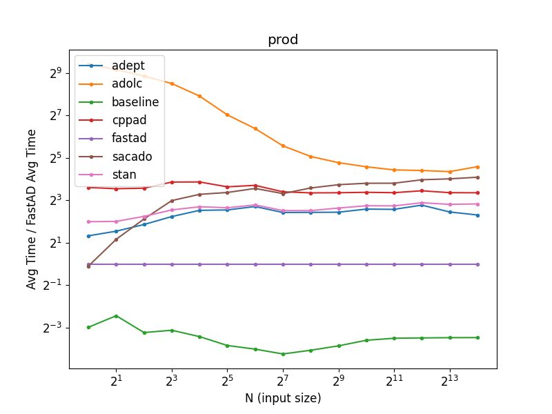
For the prod and prod iter cases, Fig. 4c,4d again show a similar trend as
sum and sum iter. Overall, the comparison with FastAD is less extreme. For
prod, Adept is about 5 times slower than FastAD, and Stan about 7 times. For
prod iter, Adept is about 3 times slower and Stan about 4.7 times.
5.2 Log-Sum-Exp
n
The log-sum-exp function is defined as f : Rn → R where f (x) = log( exi ),
P
i=1
Fig. 5 shows the benchmark results.14 J. Yang
Fig. 5: Log-sum-exp benchmark of other libraries against FastAD plotted relative
to FastAD average time.
FastAD outperforms all libraries for all values of N . The next three fastest
libraries are Adept, Stan, and CppAD, respectively. The trend stabilizes starting
from N = 26 = 64 where Adept is about 2.5 times slower than FastAD, and Stan
about 7.7 times. Note that FastAD is only marginally slower than the baseline,
especially for small to moderate values of N , despite calls to expensive functions
like log and exp. In fact, at the largest value of N = 214 , FastAD is 1.5 times
slower than the baseline, meaning there is about 50% overhead from one forward-
evaluation to also compute the gradient. This is because FastAD is optimized
such that in this case the forward-evaluated result for exp expression is reused
during the backward-evaluation.
5.3 Matrix Multiplication
For this benchmark, all matrices are square matrices of the same size. In order
to have a scalar target function, we add another step of adding all of the entries
of the matrix multiplication, i.e.
K X
X K
f (A, B) = (A · B)ij
i=1 j=1
Fig. 6 shows the benchmark results.
FastAD is still the fastest library for all values of N , but Stan performs much
closer to FastAD than in the previous examples. All other libraries consistentlyFastAD: C++ Template Library for AD 15
Fig. 6: Matrix multiplication benchmark of other libraries against FastAD plot-
ted relative to FastAD average time.
take longer than both FastAD and Stan as N increases. Towards the end at
around N = 214 , Stan is about 2 times slower. For moderate sized N ∈ [28 , 210 ],
Stan is about 3 times slower.
This example really highlights the benefits of vectorization. As noted in Sec-
tion 4.1, this was the one benchmark example where Stan was able to produce
vectorized code, which is consistent with Figure 6 that Stan is the only library
that has the same order of magnitude as FastAD. Other libraries did not produce
vectorized code.
The comparison with the baseline shows that FastAD takes 3.27 times longer.
Note that forward-evaluation requires one matrix multiplication between two
K × K matrices, and backward-evaluation additionally requires two matrix mul-
tiplications of the same order, one for each adjoint:
∂f ∂f ∂f ∂f
= · BT , = AT ·
∂A ∂(A · B) ∂B ∂(A · B)
Hence, in total, one AD evaluation requires three matrix multiplications between
two K ×K matrices. If we approximate a manually-written gradient computation
to take three times as long as the baseline (one multiplication), FastAD time
relative to this approximated time is 3.27
3 = 1.09. This shows then that FastAD
only has about 9% overhead from a manually-written code, which is extremely
optimal.16 J. Yang
Fig. 7: Normal log-pdf benchmark of other libraries against FastAD plotted rel-
ative to FastAD average time.
5.4 Normal Log-PDF
The normal log-pdf function is defined up to a constant as:
N
1 X 2
f (x) = − (xi − µ) − N log(σ)
2σ 2 i=1
For this benchmark, µ = −0.56, σ = 1.37 and are kept as constants. Fig. 7 shows
the benchmark results.
FastAD is the fastest library for all values of N . The trend stabilizes at
around N = 27 = 128. Towards the end, Adept is about 9 times slower, and
Stan about 19 times slower. Comparing all libraries, the overall difference we see
in this example is the largest we have seen so far, and this is partly due to how we
compute log(σ). Section 4.3 showed that we can check at compile-time whether
a certain variable is a constant, in which case, we can perform a more optimized
routine. In this case, since σ is a constant, it computes the normalizing constant
log(σ) once and gets reused over multiple AD evaluations with no additional
cost during runtime, which saves a lot of time since logarithm is a relatively
expensive function.FastAD: C++ Template Library for AD 17
Fig. 8: Bayesian linear regression benchmark of Stan against FastAD plotted
relative to FastAD average time.
5.5 Bayesian Linear Regression
This section marks the first macro-benchmark example. We consider the follow-
ing Bayesian linear regression model:
y ∼ N X · w + b, σ 2
w ∼ N (0, 1)
b ∼ N (0, 1)
σ ∼ U nif (0.1, 10.)
The target function is the log of the joint probability density function (up to a
constant). Fig. 8 shows the benchmark results.
FastAD outperforms Stan by 8.6 times for the largest N and Adept by 10
times. The trend stabilizes starting from around N = 70. It is interesting to see
that around N = 27 , FastAD is only 2.2 times slower than the baseline, despite
the model consisting of a large matrix multiplication and many normal log-pdfs.
One of the reasons is that the compiler was able to optimize-out the backward-
evaluation of the matrix constant X, since constants implement a no-op for
backward-evaluation.
If we assume that the most expensive operation is the matrix multiplication,
AD evaluation approximately takes two matrix multiplications between a matrix
and a vector. We can then approximate a lower bound for the manually-written
gradient computation time to be two times that of the baseline. The relative
time of FastAD to this approximated time is 1.1, implying about 10% overhead
from a manually-written code.18 J. Yang
Fig. 9: Stochastic volatility benchmark of Stan against FastAD plotted relative
to FastAD average time.
5.6 Stochastic Volatility
This section marks the second and last macro-benchmark example. We consider
the following stochastic volatility model taken from the Stan user guide [11]:
y ∼ N (0, eh )
hstd ∼ N (0, 1)
σ ∼ Cauchy(0, 5)
µ ∼ Cauchy(0, 10)
φ ∼ U nif (−1, 1)
h = hstd · σ
h[0]
h[0] = p
1 − φ2
h=h+µ
h[i] = φ · (h[i − 1] − µ), i > 0
The target function is the log of the joint probability density function (up to a
constant) and we wish to differentiate it with respect to hstd , h, φ, σ, µ. Fig. 9
shows the benchmark results.
FastAD outperforms Adept by 2 times and Stan by 2.6 times for the largest
N . The trend seems to stabilize starting from N = 210 . It is interesting to see
that FastAD actually performs better than the baseline for moderate to largeFastAD: C++ Template Library for AD 19 N values. For a complicated model as such, there are many opportunities for FastAD to cache certain evaluations for constants as mentioned in Section 4.3 and 5.4. In particular, the exponential function eh reuses its forward-evaluated result, and many log-pdfs cache the log of its parameters such as log(σ) in the Normal log-pdfs and log(γ) in the Cauchy log-pdfs (σ, γ are the second parameters of their respective distributions, which are constant in this model). Note that this caching is automatically done in FastAD, which would be tedious to manually code for the baseline. Hence, this shows that due to automatic caching, FastAD forward and backward-evaluation combined can be faster than a manually-written forward evaluation only, which puts FastAD at an optimal performance. 6 Conclusion In this paper, we first introduced the reverse-mode automatic differentiation al- gorithm to give context and background on how FastAD is implemented. We then discussed how FastAD uses vectorization to boost the overall performance, expression template and lazy allocation strategies to simplify memory manage- ment, and compile-time checks to further reduce run-time. To see how FastAD performs in practice, we rigorously benchmarked a set of micro and macro- benchmarks with other popular C++ AD libraries and showed that FastAD consistently achieved 2 to 19 times faster speed than the next two fastest li- braries across a wide range of examples. 7 Further Studies FastAD is still quite new and does not have full support for all commonly-used functions, probability density functions, and matrix decompositions. While Fas- tAD is currently optimized for CPU performance, its design can also be extended to support GPU. Having support for both processors will allow FastAD to be well-suited for extremely large-scale problems as well. Although computing hes- sian would be easy to implement in FastAD, generalizing to higher-order deriva- tives seems to pose a great challenge, and this feature could be useful in areas such as physics and optimization problems. Lastly, one application that could potentially benefit greatly from FastAD is probabilistic programming language such as Stan, which heavily uses automatic differentiation for differentiating scalar functions. 8 Acknowledgements We would like to give special thanks to the members of the Laplace Lab at Columbia University, especially Bob Carpenter, Ben Bales, Charles Margossian, and Steve Bronder, as well as Andrea Walther, Eric Phipps, and Brad Bell, the maintainers of ADOL-C, Sacado, and CppAD, respectively, for their helpful
20      J. Yang

comments on the first draft and for taking the time to optimize the benchmark
code for their respective libraries. We also thank Art Owen and our colleagues
Kevin Guo, Dean Deng, and John Cherian for useful feedback and corrections
on the first draft.

References
 1. Bartlett, R.A., Gay, D.M., Phipps, E.T.: Automatic differentiation of c++ codes
    for large-scale scientific computing. In: Alexandrov, V.N., van Albada, G.D., Sloot,
    P.M.A., Dongarra, J. (eds.) Computational Science – ICCS 2006. pp. 525–532.
    Springer Berlin Heidelberg, Berlin, Heidelberg (2006)
 2. Bell, B.: Cppad: a package for c++ algorithmic differentiation http://www.coin-or.
    org/CppAD
 3. Carpenter, B., Hoffman, M.D., Brubaker, M., Lee, D., Li, P., Betancourt, M.: The
    stan math library: Reverse-mode automatic differentiation in c++ http://arxiv.
    org/abs/1509.07164v1
 4. Goodfellow, I., Bengio, Y., Courville, A.: Deep Learning, chap. 6.5 Back-
    Propagation and Other Differentiation Algorithms, p. 200–220. MIT Press (2016)
 5. Griewank, A., Walther, A.: Evaluating Derivatives: Principles and Techniques
    of Algorithmic Differentiation. Society for Industrial and Applied Mathematics
    (SIAM), 2 edn. (2008)
 6. Griewank, A., Juedes, D., Utke, J.: Algorithm 755: Adol-c: A package for the
    automatic differentiation of algorithms written in c/c++. ACM Trans. Math.
    Softw. 22(2), 131–167 (Jun 1996). https://doi.org/10.1145/229473.229474, https:
    //doi.org/10.1145/229473.229474
 7. Hoffman, M.D., Gelman, A.: The no-u-turn sampler: Adaptively setting path
    lengths in hamiltonian monte carlo http://arxiv.org/abs/1111.4246v1
 8. Hogan, R.J.: Fast reverse-mode automatic differentiation using expression tem-
    plates in c++ 40 (2014)
 9. Margossian, C.C.: A review of automatic differentiation and its efficient implemen-
    tation http://arxiv.org/abs/1811.05031v2
10. Neal, R.M.: Handbook of Markov Chain Monte Carlo, chap. 5: MCMC Using
    Hamiltonian Dynamics. CRC Press (2011)
11. Team, S.D.: Stan modeling language users guide and reference manual (2018),
    http://mc-stan.org
12. Vandevoorde, D., Josuttis, N.M.: C++ Templates: The Complete Guide. Addison-
    Wesley, 2 edn. (2002)
You can also read