Granger causality analysis of deviation in total electron content during geomagnetic storms in the equatorial region - Journal of Engineering and ...
←
→
Page content transcription
If your browser does not render page correctly, please read the page content below
Iyer and Mahajan Journal of Engineering and Applied Science                 (2021) 68:4
https://doi.org/10.1186/s44147-021-00007-x
                                                                                                                              Journal of Engineering
                                                                                                                              and Applied Science

 RESEARCH                                                                                                                                        Open Access

Granger causality analysis of deviation in
total electron content during geomagnetic
storms in the equatorial region
Sumitra Iyer1*        and Alka Mahajan2

* Correspondence:
sumitraiyer2017@gmail.com                Abstract
1
 Department of Electronics and
Communication, Nirma Institute of        The total electron content (TEC) in the ionosphere widely influences Global Navigation
Technology, Ahmedabad, Gujarat,          Satellite Systems (GNSS) especially for critical applications by inducing localized positional
India                                    errors in the GNSS measurements. These errors can be mitigated by measuring TEC from
Full list of author information is
available at the end of the article      stations located around the world at various temporal and spatial scales and using them for
                                         advanced forecasting of TEC. The TEC can be used as a tool in understanding space
                                         weather phenomena such as geomagnetic storms which cause disruptions in the
                                         ionosphere. This paper examines the causal relationship between perturbations in TEC
                                         caused by geomagnetic storms. The causality between two geomagnetic indices auroral
                                         electrojet (AE) and disturbed storm index (Dst) and TEC is investigated using Granger
                                         causality at two low-latitude stations, Bangalore and Hyderabad. The outcomes of this study
                                         strengthen the regional understanding and modeling of ionospheric parameters which can
                                         contribute towards the global efforts for modeling and reducing the ionospheric effects on
                                         trans-ionospheric communication and navigation. The causal inferences combined with the
                                         data-driven model can be useful in identifying the correct and informative physical
                                         quantities to improve the forecasting models.
                                         Keywords: Geomagnetic storm, Ionosphere, Total electron content, Global Positioning
                                         System, Granger causality, Cointegration

                                       Introduction
                                       The changes in the solar wind and interplanetary medium’s physical conditions due to
                                       the solar activity result in several space weather phenomena such as geomagnetic
                                       storms and substorms which causes large magnetic field perturbations and distur-
                                       bances in the near-Earth environment [1]. The technologies, such as the Global Posi-
                                       tioning System (GPS), which play an important role in navigation, are severely affected
                                       by these disturbances. Therefore, it is important to mitigate the damages and errors
                                       caused due to these phenomena. Also, it is necessary to get a deeper knowledge of the
                                       physical processes responsible for generating such disturbances in the near-Earth en-
                                       vironment and model and forecast their complex behavior. This is attempted by inves-
                                       tigating dependencies between the parameters defining the geomagnetic storms
                                      © The Author(s). 2021 Open Access This article is licensed under a Creative Commons Attribution 4.0 International License, which
                                      permits use, sharing, adaptation, distribution and reproduction in any medium or format, as long as you give appropriate credit to the
                                      original author(s) and the source, provide a link to the Creative Commons licence, and indicate if changes were made. The images or
                                      other third party material in this article are included in the article's Creative Commons licence, unless indicated otherwise in a credit
                                      line to the material. If material is not included in the article's Creative Commons licence and your intended use is not permitted by
                                      statutory regulation or exceeds the permitted use, you will need to obtain permission directly from the copyright holder. To view a
                                      copy of this licence, visit http://creativecommons.org/licenses/by/4.0/. The Creative Commons Public Domain Dedication waiver
                                      (http://creativecommons.org/publicdomain/zero/1.0/) applies to the data made available in this article, unless otherwise stated in a
                                      credit line to the data.
Iyer and Mahajan Journal of Engineering and Applied Science        (2021) 68:4                                Page 2 of 25

                 namely disturbed storm index (Dst) and auroral electrojet index (AE) and the TEC
                 which defines the dynamics of the ionosphere which impacts the positional accuracy.
                 The causality between the variables is evaluated in this study. The details about the
                 ionosphere TEC and geomagnetic indices are explained in the next section.

                 Ionosphere
                 The ionosphere is a region in the upper atmosphere which extends from around 50 to
                 1000 km height and is characterized by partially ionized plasma [2]. The ionosphere is
                 described by the TEC in the layer. The TEC is the total number of electrons present
                 along a path between a radio transmitter and receiver. It is measured in electrons per
                 square meter. By convention, 1 TEC Unit or 1 TECU = 1016 electrons/m2.
                   The TEC is estimated from Global Navigation Satellite System (GNSS) observables
                 and is an important tool in studying the space weather impacts. The TEC in the iono-
                 sphere depends on the solar activity like solar flares, coronal mass ejections, high-speed
                 solar wind, solar cycle, solar maxima, and minima. As these solar activities vary with
                 time and have different impacts at different locations, therefore, the TEC also varies
                 due to local time, latitude, longitude, season, geomagnetic conditions, and solar cycle
                 and exhibits temporal and spatial variation. The TEC is found to be maximum near the
                 equator and tapering at poles. The seasonal effects are also observed in TEC due to the
                 movement of the Earth around the Sun. Furthermore, the electron density is linked to
                 the 11-year solar cycle, and during this cycle, it goes through a maximum when the
                 ionosphere is more likely to be disturbed, and the electron density much higher and
                 unpredictable as compared to a quiet day [3]. The daily distribution of TEC also fre-
                 quently gets affected by geomagnetic storms, during the high solar activity period.
                   The ionosphere attributes to one of the largest errors in GPS positioning. Apart from
                 positional error, the ionosphere also causes Faraday rotation and bending of radio
                 waves of GPS signal. The irregularity in the ionosphere also leads to rapid fluctuations
                 in signal amplitude/phase or scintillations. The dispersive nature of the ionosphere adds
                 to the complexity and makes the positional error dependent on the frequency of the in-
                 coming signal [4]. This dependence is described in Eq. 1 and is obtained from the Ap-
                 pleton and Hartree general equation for the ionosphere’s refractive index [5].

                                                        2
                                1           f plasma                       N
                      niono ¼ 1−                             ¼ 1−40:3                                ð1Þ
                                2             f signal                     f2

                 where niono is the refractive index, fplasma the plasma frequency, N is the electron dens-
                 ity, and fsignal is the incoming signal frequency. This Eq. 1 is modified and used to
                 evaluate the group delay of a ray path crossing the ionosphere, which is given by Eq. 2

                                     TEC
                      y1 ¼ 40:3                                                                       ð2Þ
                                     f signal2

                    For a single-frequency receiver on L1 frequency, positional error due to group delay
                 is minimized using a correction code. This code emulates the spatial and temporal vari-
                 ations and is broadcasted to the receivers. Several models have been proposed and the
                 Klobuchar model is being currently used in GPS receivers. However, in a dual-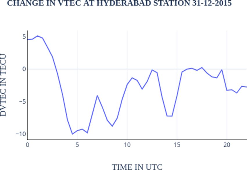
Iyer and Mahajan Journal of Engineering and Applied Science   (2021) 68:4                                     Page 3 of 25

                 frequency receiver, the TEC is computed at two different frequencies and error is elimi-
                 nated [6]. The TEC estimation for a dual-frequency receiver at L1 and L2 frequencies is
                 shown in Eq. 3 where L1 is given as 1575.42 MHz and L2 1227.6 MHz and P1 and P2
                 are group path lengths.


                             1 L12 :L22
                      TEC ¼                 ðP1−P2Þ                                                    ð3Þ
                            40:3 L12 −L22

                   Thus, TEC is an important parameter to understand the dynamics of the ionosphere.
                 The TEC has a linear relationship with the positional error and 1 TECU of electron
                 content produces a range error of 0.16 m at L1 frequency [7].
                   The ionosphere is one of the largest obstacles for the Global Positioning System
                 (GPS) to become the primary navigational aid for critical applications and can cause
                 positioning errors, which may be more than 50 m. As seen above, these errors can be
                 eliminated in dual-frequency receivers. However, for single-frequency receivers, these
                 errors can be only reduced by applying fixed corrections based on GNSS observables.
                 For equatorial regions, due to equatorial anomaly and complex spatio-temporal varia-
                 tions in TEC, furthermore, the space weather phenomena like geomagnetic storms
                 cause unpredictable irregularities in the ionosphere causing deviation in TEC pattern.
                 Although there are several geomagnetic indices available to explain the strength of the
                 geomagnetic storms, they are of little use in describing the deviation in the TEC pattern
                 directly. Hence, there is a need to devise a method that can explain the impact of geo-
                 magnetic storms on TEC. This paper investigates the causality method to study the im-
                 pact of a geomagnetic storm on TEC.

                 Geomagnetic storms and geomagnetic indices
                 A geomagnetic storm is one of the major space weather activities which affects the
                 TEC and causes deviation in the TEC. A geomagnetic storm is a disturbance in the
                 magnetosphere that may cause a sudden change in electron density. The Earth’s mag-
                 netosphere, thermosphere, and ionosphere are driven by the energy emitted from the
                 Sun. The solar wind transfers its wind energy to the Earth’s magnetosphere through
                 magnetic reconnection which leads to geomagnetic storms. These slow and fast solar
                 winds from the coronal region also lead to powerful solar events like coronal mass ejec-
                 tions (CMEs) from the Sun [8] and the corotating interaction regions (CIRs). The
                 CMEs are the result of plasma outbursts from the Sun’s active region [9]. The CMEs
                 interact with the solar wind and interplanetary magnetic field of the Earth. The
                 southward-directed solar magnetic field interacts strongly with the oppositely oriented
                 magnetic field of the Earth and results in geomagnetic storms. The severe geomagnetic
                 storms lead to anomalous changes in the ionospheric TEC, resulting in frequent ampli-
                 tude and phase fluctuations. They may also cause cycle slips, amplitude, and phase
                 scintillations, or even loss of lock. Such events not only affect the determination of the
                 position of the receiver, but also the velocity and time of GPS receivers.
                   A geomagnetic storm may lead to an increase or decrease in the electron density as
                 compared to quiet days when solar and geomagnetic activities are low. Thus, a geomag-
                 netic disturbance may cause a positive ionospheric storm or a negative ionospheric
                 storm. The impact of the geomagnetic storm on TEC depends on the phase and origin
Iyer and Mahajan Journal of Engineering and Applied Science (2021) 68:4 Page 4 of 25
of the storm. A positive ionospheric storm is seen during the main phase, while in the
recovery phase, negative storms are pronounced at all latitudes [10]. Positive storm ef-
fects with enhanced TEC are observed at geomagnetically low and mid-latitudes in the
daytime, and negative storm effects are observed near the geomagnetic equator [11].
The TEC in the equatorial region is also impacted by the equatorial anomaly, which
causes TEC accumulation at certain latitudes due to the formation of crests. This is pri-
marily due to the equatorial electrojet (EEJ), which is caused due to vertical EXB drift
leading to the fountain effect. The entire phenomenon is dependent on the EEJ and found
to be more pronounced during the high solar activity period or equinox months. Hence,
the geomagnetic storm effects are far more pronounced in the equatorial regions.
The strength and impact of geomagnetic disturbances are estimated using geomag-
netic indices like Kp, Dst, and AE, to name a few [12]. In this study, two indices AE
and Dst are selected. Both the indices are available at 1-h interval while Kp index is a
3-hourly index. Furthermore, there is a good correlation between Dst and AE; hence,
AE and Dst are selected for the study. The magnitude of these indices is determined
using the horizontal H component of the geomagnetic field. These indices have a pat-
tern characteristic pattern during quiet and disturbed conditions.
The AE index characterizes the intensity of the auroral zone currents or auroral elec-
trojet. It is the difference between the largest negative and positive H component varia-
tions, the AL and AU indices. The AE index uses magnetograms of the H component.
This is collected from twelve observatories located over the longitude in the northern
hemisphere at auroral or subauroral latitudes [13]. In a quiet time, this index’s value is
tens of nT, and during storms and substorms, it increases to several hundred and more
than a thousand nano-Tesla (nT).
The Dst index is the globally averaged value of the horizontal component of the Earth’s
magnetic field at the magnetic equator from a few magnetometer stations [14]. The Dst is
computed once per hour and reported in near-real-time. During quiet times, the Dst value
is between + 20 and − 20 nT. Based on a geomagnetic storm’s strength, it can be classified
as a moderate storm for Dst between − 50 and − 100 nT, intense for Dst between − 100
and − 200 nT, and severe or super-storm for Dst less than − 200 nT [15].
In the proposed work, an attempt is made to see if TEC can be used to study and under-
stand the impact of space weather phenomena. This study of the dependency of TEC on AE
and Dst indices can be helpful to understand the impact of space weather phenomena on the
satellite-based system. The advantage of using TEC is its high temporal resolution as com-
pared to other indices used for measuring geomagnetic storms like Dst and AE, which are
available at 1-h intervals, or Kp, which is available at 3-h intervals. Furthermore, the equatorial
ionosphere is characterized by large ionospheric gradients (even within 5°X 5° latitude and
longitude). The deviations and perturbations in the TEC at different latitudes due to geomag-
netic storms are also different. Thus, investigating the causality between the geomagnetic
storm and TEC at the regional level can be useful in improving the existing methods used for
correcting positional errors. This can be achieved with the high spatial resolution regional
TEC data available from the GNSS receivers which have a wide global coverage. As causal in-
ferences can result in the selection of physical quantities which are more informative, hence,
the proposed study can be further combined with data-driven models for improved estimation
of positional forecasting errors in the propagating signal.Iyer and Mahajan Journal of Engineering and Applied Science (2021) 68:4 Page 5 of 25
Granger causality test
Causality refers to the dependency between variables and is different from correlation.
Although there is a well-known correlation between variation in TEC during the occur-
rence of geomagnetic storms and substorms, there is no clear, direct cause and effect
relation between them which can be modeled to forecast TEC.
Several attempts to forecast TEC using geomagnetic disturbances (in terms of both
geomagnetic indices AE and Dst measurements) during magnetic storms and sub-
storms have been developed using Artificial Neural Networks and linear or nonlinear
regression models [16, 17]. However, most of these models are based on using a large
historical dataset of these physical quantities. Many feature selection methods have also
been combined with these models to identify the most relevant physical quantity. How-
ever, there is little work done in the area to identify the most informative physical
quantities. Most of the studies are based on the correlation between the physical quan-
tities which may not be very indicative due to the nonlinear and abrupt nature of these
variations [18].
In a stochastic system, Granger causality between the variables can be established if it is
possible for variable Xt to cause Yt + 1 or for Yt to cause Xt + 1 where t is the time variable
[19]. This paper investigates the causality between the variables—deviation in TEC, Dst,
and AE. The Granger causality test or G test method proposed by the Nobel Economics
Prize recipient Clive W. J. Granger is used to analyze the causality between the variables.
For a time series, the Granger causality is said to exist between two variables, X and
Y, if variable X can help explain Y’s future values, considering both time series are sta-
tionary or steady. Therefore, before conducting the Granger causality test, it is neces-
sary to conduct a unit root test of the time series’ stationarity, which ensures the
stationarity of the time series. The Augmented Dickey-Fuller test (ADF test) is gener-
ally used to conduct this unit root test of stationarity of the series. The Granger causal-
ity is sensitive to the lag period, and under different lag periods, completely different
test results can be obtained if a precondition of stationarity is not satisfied. Thus, a
series of pretests must be performed on the data before the G test.
In the present study, the deviation in TEC denoted by DTEC is taken as Y or the
dependent variable, and Dst or AE are explanatory variables X1 and X2. The causality
test is performed to check if AE/Dst can cause deviation in TEC. Hence, if X1/X2 does
not help predict variable Y, which is DTEC, then X1/X2 is not the cause for the devi-
ation in TEC. On the contrary, if the Dst or AE is the cause for DTEC, then AE and
Dst should be able to predict the variable DTEC. A statistical hypothesis is tested to es-
tablish the causality. This can be explained with a mathematical formulation of the test
based on vector autoregression (VAR) modeling of stochastic processes based on the
past value of two variables Y and X [20]. The regression equation for two variables can
be expressed as shown below:
X
p X
p X
p
YðtÞ ¼ A11; j Yðt−jÞ þ A12; j X1ðt− jÞ þ A13; j X2ðt− jÞ þ E 1 ðtÞ
j¼1 j¼1 j¼1
X p X p X p
X1ðtÞ ¼ A21; j Yðt− jÞ þ A22; j X1ðt− jÞ þ A23; j X2ðt− jÞ þ E 2 ðtÞ ð4Þ
j¼1 j¼1 j¼1
X
p X
p X
p
X2ðt Þ ¼ A31; j Yðt− jÞ þ A32; j X1ðt− jÞ þ A33; j X2ðt− jÞ þ E3 ðtÞ
j¼1 j¼1 j¼1Iyer and Mahajan Journal of Engineering and Applied Science (2021) 68:4 Page 6 of 25
where p is the maximum number of lagged observations; the coefficients of the model
are the contributions of each lagged observation to the predicted values of X1 (t), X2 (t),
and Y (t); and E1, E2, and E3 are residuals (prediction errors) for each time series. If the
variance of E1 (or E2/E3) is reduced by the inclusion of the Y (or X) terms in the equa-
tion, then it is said that Y (or X) Granger-(G)-causes X (or Y). In other words, Y G-
causes X if the coefficients in Aij are significantly different from zero. This is tested by
performing a t-test or chi-squared test of the null hypothesis that Aij = 0, given as-
sumptions of covariance stationarity on X and Y.
Cointegration
The cointegration test is done to establish the presence of a statistically significant con-
nection between two or more time series. It is seen that if two variables are cointe-
grated, then there exists causality between variables in at least one direction [21]. Thus,
a cointegration test can be viewed as an indirect test of long-run dependence. It occurs
when two or more non-stationary time series have a long-run equilibrium and move
together so that their linear combination of variables results in a stationary time series.
There is a linear combination of the variables with an order of integration less than that
of the individual series. In this context, cointegration can help understand if there is a
long-run equilibrium between deviation in TEC during the disturbed condition and
Dst/AE. The cointegration test establishes a stationary linear combination of time series
that are not themselves stationary.
Thus, the cointegration test indicates a long-run equilibrium relationship between
variables, while the Granger causality test indicates a unidirectional causality. The re-
sults of cointegration determine the type of regression model to be implemented for
the causality test. The regression results with non-stationary variables can be spurious
if the variables are non-stationary and cointegrated. Furthermore, the regression with
the first differenced variables is for short-run relationship; hence, it cannot capture the
long-run information. In such cases, the causality is investigated through vector error
correction model (VECM). It is an extension of the VAR model to include cointegrated
variables that balance the short-term dynamics of a process with the long-term depend-
encies. The VECM expresses the long-run dynamics of the process including error cor-
rection terms that measure the deviation from the stationary mean at (t−1) time. Thus,
linear Granger causality on VAR can be applied only to time series that are stationary.
If data are not stationary and not cointegrated, then the VAR can fit to the differenced
time series. For a cointegrated non-stationary time series, with a long-term equilibrium
relationship, the time series have to be fitted with the VECM model to evaluate the
short-run properties of the cointegrated time series.
In this paper, three variables namely deviation in TEC, Dst, and AE are investigated
under different storm conditions and for two different locations in the equatorial re-
gion. The primary aim is to identify the extent of causality and identify causal variables
that can cause a state transition. As per the Granger causality principles [22], forecast-
ing is related to identifying causal variables responsible for state transitions. Therefore,
Granger causality inferences between variables can be combined with forecasting and
can improve forecasting.Iyer and Mahajan Journal of Engineering and Applied Science (2021) 68:4 Page 7 of 25
Methods
The data used for the study is from the year 2015 which is the descending phase of the
24th solar cycle. The year 2015 is characterized by 56 geomagnetic storms, of which
the storm on March 17, 2015, was the most severe one (St. Patrick’s storm) of the solar
cycle [23]. This storm had major adverse effects on communication and navigation sys-
tems on and above the Earth. The present study is conducted with thirty geomagnetic
storms. In this paper, twelve geomagnetic storms are presented, which is used to verify
the causal effect of geomagnetic indices on ionospheric TEC measured at two different
GPS stations at Bangalore and Hyderabad. The geographic and geomagnetic coordi-
nates (latitudes and longitudes) of the GPS stations are given in Table 1.
The storms considered for this study are of different intensities and of different types
and origins (recurrent and sporadic). The details of the storm durations, storm type,
geomagnetic indices (Dst and AE), and TEC characteristics are listed in Table 2. The
maximum TEC values for all storm days are higher than the quiet day maximum TEC
value. Furthermore, the maximum value of TEC is observed to be higher at Hyderabad
due to the crest formation around noon time.
Data preparation
For this study, three parameters namely deviation in TEC denoted by “DTEC” and the
geomagnetic storm indices “Dst” and AE” are used. Both Dst and AE are available at 1-
h time interval and DTEC is available at 2.5-minute interval. The DTEC is calculated
from the vertical total electron content (VTEC) for which the calculation is shown in
the next section. The descending phase of the twenty-fourth cycle is chosen and the
VTEC data of geomagnetic storm days occurring in this period is considered for this
study. The storm days are selected based on the Dst index.
Calculation of VTEC
The VTEC is the vertical total electron content and is computed from the receiver in-
dependent exchange (RINEX) observation files of the International GNSS Service (IGS)
receiver stations at Bangalore (IISC) and Hyderabad (HYDE). The data is processed
using GPS-TEC online application software, developed by Ionolab [24]. The desired
TEC is the combination of calculated TEC and receiver and satellite biases in TEC
units. The TEC is computed using the standard procedure to compute the absolute
total electron content on the slant ray path (STEC) from the satellite to the receiver
and is calculated from the difference of pseudo ranges P1 and P2 at L1 and L2 frequen-
cies respectively.
The computed slant TEC is projected to the local zenith direction to obtain the verti-
cal TEC through a mapping function, M (E, h), assuming a thin shell model of the
ionosphere. The receiver and satellite biases are also added to compute the VTEC
values. The VTEC value is computed as shown in Eq. 5:
Table 1 Locational coordinates of GPS stations
Location Geographic latitude Geographic longitude Geomagnetic latitude Geomagnetic longitude
Bangalore 13.02° N 77.57° E 4.49° N 150.93° E
Hyderabad 17.41° N 78.55° E 8.77° N 152.24° ETable 2 Details of storm days
S.N Date Storm Min Dst index Min Dst index time Max AE index Max AE index time Solar Max VTEC Occurrence Max VTEC Occurrence
type nT UT nT UT flare Storm time Storm day time
day UT Hyderabad UT
Bangalore TECU
TECU
1 01-03- Moderate −46 9 649 8 C 6.8 85.34 8 97.7 8:70
2015
2 02-03- Moderate −55 9 725 9 M1.2 83.87 10 92.7 10:30
Iyer and Mahajan Journal of Engineering and Applied Science
2015
3 17-3-2015 Severe −222 23 9781 20 M1.0 86.82 11:30 88.6 11:02
4 19-3-2015 Moderate −88 1 1134 13 C2.2 78.633 11:37 85.5 12
5 21-3-2015 Moderate −57 1 561 1 C1.7 73.64 11.04 83 10:57
(2021) 68:4
6 22-3-2015 Moderate −43 15 1078 8 C1.3 82.41 10:47 92.52 10:52
7 16-4-2015 Moderate −79 23 1082 21 C5.7 90 9.5 110 10
8 22-6-2015 Severe −121 22 1636 19 M6.6 42.5 8 42.5 8
9 23-6-2015 Intense −204 5 614 2 C1.9 55 13 55.5 13
10 20-12- Intense −155 22 1396 13 C6.0 52.5 8 52.5 9
2015
11 21-12- Moderate −148 2 681 1 M2.8 45.5 9 45 8
2015
12 31-12- Moderate −93 23 1373 13 B2.8 42.5 9 48 9
2015
Page 8 of 25Iyer and Mahajan Journal of Engineering and Applied Science (2021) 68:4 Page 9 of 25
TEC slant ðSTECÞ ¼ M ðE; hÞ TEC vertical ðVTECÞ
" #−1=2
R cosðEÞ 2 ð5Þ
where M ðE; hÞ ¼ 1−
Rþh
In the above formula, R is the radius of the Earth, E is the elevation angle, and h is
the height of the ionospheric pierce point.
Calculation of deviation in TEC (DTEC)
The DTEC is the deviation in TEC on a geomagnetic storm day w.r.t. the TEC on a
quiet day. For this calculation, the quietest day of the month is selected to be used as
the reference TEC pattern for that month. Monthly selection is done to take care of
seasonal variations in TEC. The quiet day is selected based on the Dst and Kp indices.
The quiet days selected for every month have low solar and geomagnetic activities such
that Dst variation does not exceed 5 to 10 nT over the entire day and the absolute
value is also within −15 to 15nT. The DTEC is computed as a deviation in TEC, as
shown in Eq. 6
DTEC ¼ TEC storm - TEC quiet ð6Þ
The DTEC is the measure of deviation in TEC caused due to disturbed geomagnetic
storm conditions over the entire day. Figure 1 shows the comparison of the VTEC vari-
ation pattern for a quiet day on March 10, 2015, and a moderate geomagnetic storm
day on March 2, 2015, at Hyderabad. Similarly, Fig. 2 shows the variation for Bangalore
station for a quiet day on March 10, 2015, and a geomagnetic storm day on March 2,
2015. Figures 3 and 4 show the plot of DTEC for March 2, 2015, for both Hyderabad
and Bangalore. In the equatorial region, the TEC pattern shows latitudinal variation
which can be seen in Figs. 1 and 2. Hence, DTEC is also different for both the latitudes.
The geomagnetic storm that occurred on March 17, 2015, is considered the most in-
tense storm of the solar cycle. Hence, the TEC pattern also shows a steep rise in TEC
around 5 UTC. This can be seen in Figs. 5 and 6 which represent the comparison of
variation pattern between quiet day (10-3-2015) and severe geomagnetic storm day on
March 17, 2015, for Hyderabad and Bangalore stations, respectively. Figures 7 and 8
show the DTEC for March 17, 2015, for Hyderabad and Bangalore, respectively, which
is different from the DTEC on March 2, 2015. Major variation in the TEC pattern is
generally seen on severe storm days while the minor variation pattern is observed for
moderate storm days.
The figures clearly indicate that the deviation pattern also varies with latitude. The
DTEC is more abrupt during days having the main phase of intense/severe storms (17-
3-2015). This is further verified from Figs. 9 and 10 which show deviation in TEC for
another severe storm day that occurred June 22, 2015. Figures 11 and 12 are the DTEC
variation on a moderate storm day, Dec 31, 2015, where rapid variations of smaller
magnitudes are seen.
Data for Dst and AE indices
The data for the DST index and AE index are downloaded from data centers for geo-
magnetism, Kyoto website (http://wdc.kugi.kyoto-u.ac.jp). Both indices describe theIyer and Mahajan Journal of Engineering and Applied Science (2021) 68:4 Page 10 of 25
Fig. 1 VTEC quiet (10-3-2015) and moderate storm day (2-3-2015) Hyderabad
Fig. 2 VTEC quiet (10-3-2015) and moderate storm day (2-3-2015) Hyderabad moderateIyer and Mahajan Journal of Engineering and Applied Science (2021) 68:4 Page 11 of 25
Fig. 3 Deviation on moderate storm day (2-3-2015) w.r.t to quiet day (10-3-2015) Hyderabad
intensity of the storm. The variation pattern of Dst is also useful in finding the phase of
the storm. The type of the storm, sudden or recurrent, can also be deduced from the
Dst variation pattern.
A geomagnetic storm is defined by changes in the Dst index. Dst is computed once
per hour and reported in near-real-time. During quiet times, Dst is between + 20 and −
20 nano-Tesla (nT). Figure 13 shows the Dst variation on a quiet day 10-3-2015 and
Fig. 4 Deviation on moderate storm day (2-3-2015) w.r.t to quiet day (10-3-2015) BangaloreIyer and Mahajan Journal of Engineering and Applied Science (2021) 68:4 Page 12 of 25
Fig. 5 VTEC quiet (10-3-2015) and severe storm day (17-3-2015) Hyderabad intense
Fig. 6 VTEC quiet (10-3-2015) and severe storm day (17-3-2015) HyderabadIyer and Mahajan Journal of Engineering and Applied Science (2021) 68:4 Page 13 of 25
Fig. 7 Deviation on severe storm day (17-3-2015) w.r.t to quiet day (10-3-2015) Hyderabad
19-1-2015. These days have also been used as reference days in this study. The vari-
ation is between 1 and 10 nT on 10-3-2015 and between −10 and 10 nT on 19-1-2015.
Most of the geomagnetic storms have three phases: initial, main, and recovery. The
initial phase is characterized by an increase in Dst by 20 to 50 nT in a short time. The
initial phase is also referred to as a storm sudden commencement (SSC). This is
followed by the main phase characterized by Dst decreasing to less than −50 nT. The
Fig. 8 Deviation on severe storm day (17-3-2015) w.r.t to quiet day (10-3-2015) BangaloreIyer and Mahajan Journal of Engineering and Applied Science (2021) 68:4 Page 14 of 25
Fig. 9 Deviation on severe storm day (22-6-2015) w.r.t to quiet day (10-3-2015) Hyderabad
minimum value during a storm can range from −50 to −600nT in extreme cases. The
duration of the main phase is typically 2–8 h. The recovery phase is when Dst changes
back from its minimum value to its quiet time value. The recovery phase may range
from 8 h to 7 days. However, not all geomagnetic storms have an initial phase and not
all sudden increases are followed by a geomagnetic storm. Figure 14 shows the Dst
variation of severe geomagnetic storm day on 17-3-2015 and a moderate storm day on
Fig. 10 Deviation on severe storm day (22-6-2015) w.r.t to quiet day (10-3-2015) BangaloreIyer and Mahajan Journal of Engineering and Applied Science (2021) 68:4 Page 15 of 25
Fig. 11 Deviation on moderate storm day (31-12-2015) w.r.t to quiet day (10-3-2015) Hyderabad
31-12-2015 considered during this study. The Dst variation on 17-3-2015 indicates the
rising Dst in the initial phase and Dst reaching its minimum (−220 nT) in the main
phase of the storm. The moderate storms are many times recurrent and periodic in na-
ture with a gradual decrease in Dst. The Dst pattern is more predictable. Sometimes,
substorms are triggered during the recovery phase of intense storms.
Fig. 12 Deviation on moderate storm day (31-12-2015) w.r.t to quiet day (10-3-2015) BangaloreIyer and Mahajan Journal of Engineering and Applied Science (2021) 68:4 Page 16 of 25
Fig. 13 Diurnal pattern of Dst variation on a quiet day
The AE index represents the auroral zone magnetic activity produced by enhanced
ionospheric currents flowing below and within the auroral oval. The equatorward ex-
pansion of auroral electrojet influences the TEC in the low-latitude ionosphere. They
have been useful in studying the magnetic substorms. The enhancement in AE can be
seen on days with high geomagnetic activity. Figure 15 shows the AE index for quiet
and storm days. The quiet days on 10-3-2015 show two peaks of 200nT and for most
of the day the value is not more than 50 nT. The AE index ranges between 50 and
200nT on 19-1-2015. Two storm days one severe (17-3-2015) and one moderate (31-
12-2015) are shown in Fig. 15. On both days, the TEC is enhanced to around 1500nT
and for most of the day, it is more than 500nT.
Data scaling
All the geomagnetic indices and DTEC are normalized using the Min-Max scaler
method. The Min-Max scaler is chosen as it preserves the original distribution’s shape
and does not change the meaning of the information embedded in the original data.
Results and discussion
In this section, the results for twelve different geomagnetic storms of different origins
and types are presented. The year 2015 had a total of 56 storms out of which 52 were
of low or moderate intensity, 2 were intense, and 2 were severe. In this paper, the test
results for two severe storms and two intense storms and 8 moderate storms are pre-
sented. The tests have been conducted for thirty storm days at both Bangalore and
Fig. 14 Diurnal pattern of Dst variation on a moderate storm day and severe storm day on 17-3-2015Iyer and Mahajan Journal of Engineering and Applied Science (2021) 68:4 Page 17 of 25
Fig. 15 Diurnal pattern of AE variation on quiet day and enhancement on moderate storm day (31-12-
2015) and severe storm day (17-3-2015)
Hyderabad stations as TEC data was not available for some of the disturbed days. Three
tests namely the Augmented Dickey-Fuller Test, Granger causality test, and cointegra-
tion test are carried out. All the tests are performed on normalized data. First, the sta-
tionarity of raw data is tested. The stationarity is tested using the Augmented Dickey-
Fuller Test (ADF test). The Granger causality test is performed on the stationary data.
The causality between the variables and the direction of the causality is tested using the
Granger causality test. The long-term equilibrium relationships between variables are
tested using the cointegration test. The detailed observations are presented below.
Stationary test of variables
All the three time-series data are first tested for trend and stationarity. Differencing
technique is used for making the data stationary. The stationarity is tested after every
differencing. The differenced data’s stationarity is tested after single and double (if re-
quired) differencing using the Augmented Dickey-Fuller Test (ADF test). The test uses
the null hypothesis: “Data has a unit root and is non-stationary” is tested. The test is
performed for different lag values with a 0.05 significance value. The p value is used to
decide if there is any evidence to reject the null hypothesis. This test is repeated for all
the data variables.
Cointegration test
Johansen cointegration test is performed on data to establish the presence of a statisti-
cally significant relationship between the time series. The Johansen method is based on
the relationship between the rank of the matrix Π and the size of its eigenvalues. The
rank of the matrix Π determines the long-term dynamics. If Π has full rank, the processIyer and Mahajan Journal of Engineering and Applied Science (2021) 68:4 Page 18 of 25
Yt is stationary in mean. If the rank of Π is zero, then the error correction term disap-
pears, and the system is stationary in differences (the VAR model in differences can be
used). If the rank of Π is r (within (0, K)), then there are r independent cointegrating
relations among the variables in Yt. For a given r, the maximum likelihood estimator of
β defines the combination of Yt − 1 that yields the r largest canonical correlations of
ΔYt with Yt − 1.
The null hypothesis “There are no cointegrating equations” is tested for a 95% confi-
dence level. If the trace statistics is greater than the critical value, then the null hypoth-
esis is rejected, establishing linear relation between the variables. Hence, for
cointegration to exist, the null hypothesis must be rejected. The cointegration test is
carried out between DTEC, Dst, and AE for all storm days. The cointegration is true
for most of the cases, and hence, there exists a long-run dependency between the vari-
ables and DTEC, AE, and Dst.
Results of the cointegration test for Bangalore
To test the null hypothesis that the variables are not cointegrated, trace and eigenvalue
statistics are carried out. For most of the cases, null hypotheses are rejected for both
eigen and trace tests. All tests are conducted with 5% critical value. Since the maximum
eigenvalue and trace test statistics values are higher than 5% critical values, the alterna-
tive of one or more cointegrating vectors is accepted.
Johansen cointegration with the hypothesis of the reduced rank of a regression coeffi-
cient matrix, estimated consistently from vector regression equations, is also tested.
Here, the maximum eigenvalue statistic and the trace statistic test the number of coin-
tegrating relations between variables. The trace test is a joint test where the null hy-
pothesis is “number of cointegrating vectors is less than or equal to r,” against a
general alternative that “there are more than r vectors,” whereas the maximum eigen-
value test conducts separate tests on the individual eigenvalues, where the null hypoth-
esis is that the “number of cointegrating vectors is r,” against an alternative of (r + 1).
Table 3 shows the cointegration results for twelve geomagnetic storm days for the
year 2015. The test is done pairwise between DTEC and Dst and DTEC and AE. For
DTEC and Dst pair, the null hypothesis is not rejected for the storm on March 19 at
the Bangalore location. For most of the storm use cases, the test statistic value is higher
as compared to the critical value for DTEC and Dst pair for Bangalore. Hence, it can
be concluded that for most of the cases the null hypothesis can be rejected. This is also
in line with the fact the geomagnetic storms can be well explained by the Dst index in
equatorial and low-latitude regions. Both the tests (eigen and trace) confirmed that
most of the storm days have cointegrating vectors indicating that the geomagnetic indi-
ces Dst and deviation in TEC have a long-run linkage at Bangalore station.
Table 4 shows the cointegration test results for DTEC and AE pair. For most of the
storm cases listed, the null hypothesis is rejected, and test statistics is higher than the
critical value except for storm that occurred on March 19, 2015, April 16, 2015, and
Jun 22, 2015. The storm on June 22 has its main phase around 20 UTC, and the AE
index shows enhancement only after 15 UT. Hence, for most of the day, the AE is low.
Similarly, the storm on April 16 is a moderate storm and the AE is almost constant at
800 nT for the entire day. The AE index is a suitable measure of substorms. It is seenIyer and Mahajan Journal of Engineering and Applied Science (2021) 68:4 Page 19 of 25
Table 3 Johansen cointegration rank test results for DTEC and Dst for the Bangalore location
S.No Storm Test using trace test statistic with 5% Test using maximum eigenvalue test
date significance level for DTEC and Dst pair statistic with 5% significance level for
DTEC and Dst pair
Rank r_ Rank r_ Test Critical Rank r_ Rank r_ Test Critical
0 1 statistic value 0 1 statistic value
1 01-03- 0 2 26.43 18.40 0 1 20.52 17.15
2015
1 2 5.908 3.841 1 2 5.908 3.841
2. 02-3- 0 2 26.43 18.40 0 1 20.52 17.15
2015
1 2 5.908 3.841 1 2 5.908 3.841
3 17-03- 0 2 28.31 18.40 0 1 21.09 17.15
2015
1 2 7.216 3.841 1 2 7.216 3.841
4 19-03- 0 2 26.84 18.40 0 1 23.38 17.15
2015
1 2 3.464* 3.841 1 2 3.464* 3.841
5 21-03- 0 2 35.20 18.40 0 1 31.71 17.15
2015
1 2 3.487 3.841 1 2 3.487 3.841
6 22-03- 0 2 34.93 18.40 0 1 28.16 17.15
2015
1 2 6.774 3.841 1 2 6.774 3.841
7 16-04- 0 2 17.88 18.40 0 1 13.50 17.15
2015
8 22-06- 0 2 33.02 18.40 0 1 28.51 17.15
2015
1 2 4.510 3.841 1 2 4.510 3.841
9 23-06- 0 2 29.29 18.40 0 1 18.78 17.15
2015
1 2 10.51 3.841 1 2 10.51 3.841
10 20-12- 0 2 35.58 18.40 0 1 23.93 17.15
2015
1 2 11.65 3.841 1 2 11.65 3.841
11 21-12- 0 2 50.48 18.40 0 2 50.48 18.40
2015
1 2 11.69 3.841 1 2 11.69 3.841
12 31-12- 0 2 27.83 18.40 0 1 21.34 17.15
2015
1 2 6.491 3.841 1 2 6.491 3.841
*Rejection of the null hypothesis at 5% level of significance
that for all cases of substorm on 21-3-2015 and 22-3-2015, the DTEC and AE reject
the null hypothesis.
Results of the cointegration test for Hyderabad
The results of Johansen’s maximum eigenvalue and trace tests for Hyderabad are given
in Tables 5 and 6. All tests are conducted with 5% critical value, since the maximum
eigenvalue and trace test statistics values are higher than 5% critical values and the al-
ternative of one or more cointegrating vectors is accepted. Table 5 shows the results
for twelve geomagnetic storm days for the year 2015. The test is done pairwise between
DTEC and Dst and DTEC and AE. Both the tests confirm that most of the storm days
under consideration have cointegrating vectors indicating that the geomagnetic indices
and deviation in TEC have a long-run linkage. Most of the storm use cases have a
higher test statistic value as compared to the critical value for DTEC and Dst pair for
Hyderabad. Hence, it can be concluded that for most of the cases the null hypothesis
can be rejected and there exists long-run cointegration.Iyer and Mahajan Journal of Engineering and Applied Science (2021) 68:4 Page 20 of 25
Table 4 Johansen cointegration rank test results for DTEC and AE pair for the Bangalore location
S.No Storm Test using trace test statistic with 5% Test using maximum eigenvalue test
date significance level for DTEC and AE pair statistic with 5% significance level for
DTEC and AE pair
Rank r_ Rank r_ Test Critical Rank r_ Rank r_ Test Critical
0 1 statistic value 0 1 statistic value
1 01-03- 0 2 39.07 18.40 0 1 34.22 17.15
2015
1 2 4.858 3.841 1 2 4.858 3.841
2. 02-3- 0 2 39.07 18.40 0 1 34.22 17.15
2015
1 2 4.858 3.841 1 2 4.858 3.841
3 17-03- 0 2 34.69 18.40 0 1 34.22 17.15
2015
1 2 6.621 3.841 1 2 4.858 3.841
4 19-03- 0 2 12.78* 18.40 0 1 9.302* 17.15
2015
5 21-03- 0 2 31.42 18.40 0 1 26.67 17.15
2015
1 2 4.748 3.841 1 2 4.748 3.841
6 22-03- 0 2 30.17 18.40 0 1 19.20 17.15
2015
1 2 10.97 3.841 1 2 10.97 3.841
7 16-04- 0 2 6.939* 18.40 0 1 6.160* 17.15
2015
8 22-06- 0 2 6.939* 18.40 0 2 6.939* 17.15
2015
9 23-06- 0 2 46.34 18.40 0 1 37.29 17.15
2015
1 2 9.050 3.841 1 2 9.050 3.841
10 20-12- 0 2 36.56 18.40 0 1 27.67 17.15
2015
1 2 8.888 3.841 1 2 8.888 3.841
11 21-12- 0 2 41.27 18.40 0 1 28.24 18.40
2015
1 2 13.03 3.841 1 2 13.03 3.841
12 31-12- 0 2 32.77 18.40 0 1 20.14 17.15
2015
1 2 12.63 3.841 1 2 12.63 3.841
*Rejection of the null hypothesis at 5% level of significance
Table 6 shows the cointegration test results for DTEC and AE pair. For most of the
storm cases, the null hypothesis is rejected. The test statistics for eigenvalue is lower
than the critical value for the storm on March 22, 2015, April 16, 2015, and Jun 22,
2015. The null hypothesis cannot be rejected for these days.
Granger causality test
The causality tests are based on the null hypothesis as follows: “Coefficients of past
values in the regression equation is zero.” Furthermore, the significance value is set (p
= 0.05) and if the p value obtained from the test is less than the significance level of
0.05, then the null hypothesis is rejected. This means that the past values of time series
(X) do not cause the series (Y) to be rejected. The hypothesis is tested using the F test.
The causality is tested pairwise. For causality to exist between the time series, the null
hypothesis must be rejected. For testing causality between DTEC and Dst and AE, the
null hypothesis is stated as “Past value of the Dst index (X1) and AE index (X2) do not
cause a deviation in VTEC (DTEC).”Iyer and Mahajan Journal of Engineering and Applied Science (2021) 68:4 Page 21 of 25
Table 5 Johansen cointegration rank test results for DTEC and Dst for the Hyderabad location
S.No Storm Trace test statistic with 5% significance Maximum eigenvalue test statistic with
date level for DTEC and Dst pair 5% significance level for DTEC and Dst
pair
Rank r_ Rank r_ Test Critical Rank r_ Rank r_ Test Critical
0 1 statistic value 0 1 statistic value
1 01-03- 0 2 29.21 18.40 0 1 22.41 17.15
2015
1 2 6.798 3.841 1 2 6.798 3.841
2. 02-3- 0 2 29.21 18.40 0 1 22.41 17.15
2015
1 2 6.798 3.841 1 2 6.798 3.841
3 17-03- 0 2 25.73 18.41 0 1 21.99 17.15
2015
1 2 3.736* 3.841 1 2 3.736* 3.841
4 19-03- 0 2 23.72 18.40 0 1 19.33 17.15
2015
1 2 4.385 3.841 1 2 4.385 3.841
5 21-03- 0 2 30.29 18.40 0 1 22.60 17.15
2015
1 2 7.693 3.841 1 2 7.693 3.841
6 22-03- 0 2 22.22 18.40 0 1 17.22 17.15
2015
1 2 4.993 3.841 1 2 4.993 3.841
7 16-04- 0 2 18.44 18.40 0 1 13.41 17.15
2015
1 2 5.032 3.841
8 22-06- 0 2 38.15 18.40 0 1 34.55 17.15
2015
1 2 3.610* 3.841 1 2 3.610* 3.841
9 23-06- 0 2 16.84 18.40 0 1 10.35 17.15
2015
10 20-12- 0 2 33.79 18.40 0 1 22.92 17.15
2015
1 2 10.87 3.841 1 2 10.87 3.841
11 21-12- 0 2 49.49 18.40 0 1 37.95 18.40
2015
1 2 11.54 3.841 1 2 11.54 3.841
12 31-12- 0 2 26.34 18.40 0 1 21.27 17.15
2015
1 2 5.066 3.841 1 2 5.066 3.841
*Rejection of the null hypothesis at 5% level of significance
Furthermore, as all the time series under consideration are non-stationary, hence the
cointegration test results are considered before performing the Granger causality test.
Hence, whenever the series are cointegrated, the causality test based on VECM is car-
ried out or else they are fitted with VAR as mentioned in the “Granger causality test”
section. The vector error correction model (VECM) expresses the long-run dynamics
of the process including error correction terms (αβ′Yt − 1) which is the measure of the
deviation from the stationary mean at time t−1 and is given as:
Y X
p−1
ΔY t ¼ c þ Y t−1 þ Γ i ΔY t−i þ ∈t ð7Þ
i¼1
P
p P
p
where Π = αβ′ and c are the drift coefficient and Π ¼ Ai−I and Γi ¼ − Aj :
i¼1 j¼iþ1Iyer and Mahajan Journal of Engineering and Applied Science (2021) 68:4 Page 22 of 25
Table 6 Johansen cointegration rank test results for DTEC and AE pair for the Hyderabad location
S.No Storm Test using trace test statistic with 5% Test using maximum eigenvalue test
date significance level for DTEC and AE pair statistic with 5% significance level for
DTEC and AE pair
Rank r_ Rank r_ Test Critical Rank r_ Rank r_ Test Critical
0 1 statistic value 0 1 statistic value
1 01-03- 0 2 35.75 18.40 0 1 30.45 17.15
2015
1 2 5.301 3.841 1 2 5.301 3.841
2. 02-3- 0 2 35.75 18.40 0 1 30.45 17.15
2015
1 2 5.301 3.841 1 2 5.301 3.841
3 17-03- 0 2 30.01 18.41 0 1 26.65 17.15
2015
1 2 3.362 3.841 1 2 3.362 3.841
4 19-03- 0 2 29.55 18.40 0 2 21.99 17.15
2015
1 2 7.557 3.841 1 2 7.557 3.841
5 21-03- 0 2 35.16 18.40 0 1 30.65 17.15
2015
1 2 4.515 3.841 1 2 4.515 3.841
6 22-03- 0 2 21.55 18.40 0 1 15.34* 17.15
2015
1 2 6.213 3.841
7 16-04- 0 2 26.35 18.40 0 1 13.80* 17.15
2015
1 2 12.56 3.841 3.841
8 22-06- 0 2 12.45* 18.40 0 1 12.38* 17.15
2015
9 23-06- 0 2 42.24 18.40 0 1 37.78 17.15
2015
1 2 4.460 3.841 1 2 4.460 3.841
10 20-12- 0 2 37.79 18.40 0 2 28.62 17.15
2015
1 2 9.172 3.841 1 2 9.172 3.841
11 21-12- 0 2 40.89 18.40 0 1 32.40 18.40
2015
1 2 8.488 3.841 1 2 8.488 3.841
12 31-12- 0 2 23.15 18.40 0 2 13.67 17.15
2015
1 2 9.476 3.841
*Rejection of the null hypothesis at 5% level of significance
If the variables in Yt have differencing order of one (I (1)), then the terms involving
differences are stationary, and the error correction term in the VEC model introduces
long-term stochastic trends between the variables.
The appropriate value of lag value p is made using the Akaike Information Criterion
(AIC). The causality result is represented as a matrix based on the p value. The
Granger causality test results on different storm days are discussed in the next section.
Results of the Granger causality test
After finding cointegration among the data series, the Granger causality is estimated
between the selected pairs DTEC and Dst and DTEC and AE. The results of the
Granger causality tests are presented in Table 7 which shows F statistics for the causal-
ity tests between variables DTEC and Dst and DTEC and AE for Bangalore. The null
hypothesis of Granger causality is rejected for most of the cases of storms and sub-
storms. This indicates that most of the geomagnetic storms can be explained by either
Dst or AE. The same procedure is repeated for Hyderabad. Table 8 summarizes theIyer and Mahajan Journal of Engineering and Applied Science (2021) 68:4 Page 23 of 25
results of the F test done for Granger causality at Hyderabad between pairs DTEC–Dst
and DTEC–AE, respectively.
For both the locations, deviation in TEC could be explained by either Dst or AE de-
pending on the nature of the storm or substorm. The difference in significance p value
between latitudes also clearly indicates that the impact of the storm is different at both
the location, and hence, this test can help in providing results at the regional level.
Conclusion
This work probes the relationship between the GPS-derived VTEC at the location and
the geomagnetic indices, Dst and AE, through causality analysis. The geomagnetic
storms can bring about a lot of irregularities in the TEC in the ionosphere causing pos-
itional errors. Hence, estimating the amount of deviation in TEC during the geomag-
netic storm can improve positional accuracy. The causal inference provides intuitive
ways for detecting an anomaly in the TEC variation during disturbed ionospheric con-
ditions. It is well known that most of the geomagnetic storms can be well explained
with Dst or AE index, and in this study, Granger causality between geomagnetic indices
and TEC could be established for most cases. As per the causality test results, causality
between deviation in TEC and both geomagnetic indices Dst and AE could not be
established simultaneously for some storms. This is primarily due to the difference in
their origin and type. However, causality could be established with either Dst or AE for
most of the storm cases tested for the year 2015. In this paper, storms of different in-
tensities, types, and different origins are presented. Some storms were in the main
phase while some of them were storms during the recovery phase. Furthermore, the
causality is tested for both recurrent and sudden commencement storms. For most of
the cases, the causality could be established with suitable lag values. The storms on
March 1 and 2 have a similar origin, and causality results are well aligned with Dst. For
most of the storm days, all three variables DTEC, AE, and Dst are found to be
Table 7 F statistics results of the Granger causality test at location Bangalore with variables DTEC
and Dst pair and DTEC and AE pair at 5% significance level
S.No Date of Null hypothesis: Dst does not Granger Null Hypothesis: AE does not Granger
the storm cause deviation in TEC cause deviation in TEC
DTEC as Y and Dst as X DTEC as Y and AE as X
p value Null hypothesis p value Null hypothesis
1 01-03-2015 0.00 Rejected 0.00 Rejected
2 02-03-2015 0.003 Rejected 0.012 Rejected
3 17-3-2015 0.019 Rejected 0.00 Rejected
4 19-3-2015 0.163* Fails to reject 0.00 Rejected
5 21-3-2015 0.049 Rejected 0.00 Rejected
6 22-3-2015 0.00 Rejected 0.00 Rejected
7 16-4-2015 0.311* Fails to reject 0.00 Rejected
8 22-6-2015 0.019 Rejected 0.129* Fails to reject
9 23-6-2015 0.816* Fails to reject 0.016 Rejected
10 20-12-2015 0.00 Rejected 0.05 Rejected
11 21-12-2015 0.00 Rejected 0.00 Rejected
12 31-12-2015 0.032 Rejected 0.548* Fails to reject
*Rejection of the null hypothesis at 5% level of significanceIyer and Mahajan Journal of Engineering and Applied Science (2021) 68:4 Page 24 of 25
Table 8 F statistics results of the Granger causality test at location Hyderabad with variables DTEC
and Dst pair and DTEC and AE pair at 5% significance level
S.No Date of Null hypothesis: Dst does not Granger Null hypothesis: AE does not Granger
the storm cause deviation in TEC cause deviation in TEC
DTEC as Y and Dst as X DTEC as Y and AE as X
p value Null hypothesis p value Null hypothesis
1 01-03-2015 0.00 Rejected 0 Rejected
2 02-03-2015 0.019 Rejected 0 Rejected
3 17-3-2015 0.085* Rejected 0.007 Rejected
4 19-3-2015 0.162* Fails to reject 0 Rejected
5 21-3-2015 0.063* Rejected 0.037 Rejected
6 22-3-2015 0.06 Rejected 0.247* Fails to reject
7 16-4-2015 0 Fails to reject 0.021 Rejected
8 22-6-2015 0.595* Rejected 0.001 Rejected
9 23-6-2015 0.002 Fails to reject 0.003 Rejected
10 20-12-2015 0.032 Rejected 0.003 Rejected
11 21-12-2015 0 Rejected 0.007 Rejected
12 31-12-2015 0.003 Rejected 0 Rejected
*Rejection of the null hypothesis at 5% level of significance
cointegrated at both the latitudes. Thus, this indicates long-run dependence in at least
one direction. The causality method can be further used for predicting the short-term
TEC irregularities by using VAR or VECM models. However, further investigation with
more variables and different lag values is required. The advance prediction of TEC can
be helpful in mitigating ionospheric effects on trans-ionospheric communication and
improve the navigation system used for critical applications especially in equatorial
regions.
Abbreviations
TEC: Total Electron Content; GNSS: Global Navigation Satellite System; AE: Auroral Electrojet; Dst: Disturbance Storm
Time; GPS: Global Positioning System; CMEs: Coronal Mass Ejection; CIRs: Corotating Interaction Region;
IMF: Interplanetary Magnetic Field; EEJ: Equatorial Electrojet; ADF: Augmented Dickey Fuller
Acknowledgements
Not applicable.
Authors’ contributions
The idea of causality is suggested by AM, and SI has implemented the idea and verified the results. All authors have
read and approved the final manuscript.
Funding
This study had no funding from any resource.
Availability of data and materials
Not applicable.
Declaration
Competing interests
The authors declare that they have no competing interests.
Author details
1
Department of Electronics and Communication, Nirma Institute of Technology, Ahmedabad, Gujarat, India. 2Mukesh
Patel School of Technology Management & Engineering, Vile Parle (West), Mumbai, India.Iyer and Mahajan Journal of Engineering and Applied Science (2021) 68:4 Page 25 of 25
Received: 25 March 2021 Accepted: 10 June 2021
References
1. Alberti T et al (2017) Timescale separation in the solar wind-magnetosphere coupling during St. Patrick’s Day storms in
2013 and 2015. J Geophys Res Space Physics 122(4):4266–4283
2. Marković M (2014) Determination of total electron content in the ionosphere using GPS technology. Geonauka 2(4):1–9
3. Panda SK, Gedam SS, Jin S (2015) Ionospheric TEC variations at low latitude Indian region. In: Satellite positioning-
methods, models and applications. Tech-Publisher, Rijeka, pp 149–174
4. Chakraborty M et al (2015) Effects of geomagnetic storm on low latitude ionospheric total electron content: a case
study from Indian sector. J Earth Syst Sci 124(5):1115–1126. https://doi.org/10.1007/s12040-015-0588-3
5. Bora S (2017) Ionosphere and radio communication. Resonance 22(2):123–133. https://doi.org/10.1007/s12045-017-0443-8
6. Ya’acob N, Abdullah M, Ismail M (2010) GPS total electron content (TEC) prediction at ionosphere layer over the
equatorial region. In: Trends in Telecommunications Technologies
7. Nayir H et al (2007) GPS/TEC estimation with IONOLAB method. 2007 3rd International Conference on Recent Advances
in Space Technologies. IEEE, Istanbul
8. Michalek G, Gopalswamy N, Xie H (2007) Width of radio-loud and radio-quiet CMEs. Sol Phys 246(2):409–414. https://doi.
org/10.1007/s11207-007-9062-y
9. Zhang J et al (2007) Solar and interplanetary sources of major geomagnetic storms (Dst≤− 100 nT) during 1996–2005. J
Geophys Res Space Physics 112(A10)
10. Jin S, Jin R, Kutoglu H (2017) Positive and negative ionospheric responses to the March 2015 geomagnetic storm from
BDS observations. J Geod 91(6):613–626. https://doi.org/10.1007/s00190-016-0988-4
11. Wang W et al (2010) Ionospheric response to the initial phase of geomagnetic storms: common features. J Geophys Res
Space Physics 115:A7
12. Kane RP (2009) Evolution of Dst and auroral indices during some severe geomagnetic storms. Rev Bras Geofísica 27(2):
151–163
13. Adebesin BO (2016) Investigation into the linear relationship between the AE, Dst and ap indices during different
magnetic and solar activity conditions. Acta Geodaetica Geophysica 51(2):315–331. https://doi.org/10.1007/s40328-015-
0128-2
14. Bergin A, Chapman SC, Gjerloev JW (2020) AE, DST and their SuperMAG counterparts: The effect of improved spatial
resolution in geomagnetic indices. J Geophys Res Space Phys 125:2020JA027828. https://doi.org/10.1029/2020JA027828
15. Bhattarai N, Narayan P Chap again, Adhikari B (2016) Total electron content and electron density profile observations
during geomagnetic storms using COSMIC satellite data. Discovery 52(250):1979–1990
16. Pallocchia G et al (2008) AE index forecast at different time scales through an ANN algorithm based on L1 IMF and
plasma measurements. J Atmos Sol Terr Phys 70(2-4):663–668
17. Camporeale E, Wing S, Johnson J (eds) (2018) Machine learning techniques for space weather. Elsevier
18. Immel TJ, Mannucci AJ (2013) Ionospheric redistribution during geomagnetic storms. J Geophys Res Space Physics
118(12):7928–7939. https://doi.org/10.1002/2013JA018919
19. Guo X, Wei B, Qihao F (2017) Granger causality test of the relationship between export and economic growth in Central
Jiangsu region. 2017 4th International Conference on Industrial Economics System and Industrial Security Engineering
(IEIS). IEEE, Kyoto
20. Seth A (2007) Granger causality. Scholarpedia 2(7):1667
21. Papana A et al (2014) Identifying causal relationships in case of non-stationary time series. Department of Economics of
the University of Macedonia, Thessaloniki
22. Granger CWJ (2004) Time series analysis, cointegration, and applications. Am Econ Rev 94(3):421–425
23. Wu CC, Liou K, Lepping RP, Hutting L, Plunkett S, Howard RA, Socker D (2016) The first super geomagnetic storm of
solar cycle 24:“The St. Patrick’s day event (17 March 2015)”. Earth Planets Space 68(1):1–12
24. Arikan FEZA et al (2008) Estimation of single station interfrequency receiver bias using GPS-TEC. Radio Sci 43(4). https://
doi.org/10.1029/2007RS003785
Publisher’s Note
Springer Nature remains neutral with regard to jurisdictional claims in published maps and institutional affiliations.You can also read