A New Model of Solar Illumination of Earth's Atmosphere during Night-Time - MDPI
←
→
Page content transcription
If your browser does not render page correctly, please read the page content below
Article
A New Model of Solar Illumination of Earth’s Atmosphere
during Night-Time
Roberto Colonna * and Valerio Tramutoli

                                          School of Engineering, University of Basilicata, 85100 Potenza, Italy; Valerio.tramutoli@unibas.it
                                          * Correspondence: roberto.colonna@unibas.it

                                          Abstract: In this work, a solar illumination model of the Earth’s atmosphere is developed. The
                                          developed model allows us to determine with extreme accuracy how the atmospheric illumination
                                          varies during night hours on a global scale. This time-dependent variation in illumination causes a
                                          series of sudden changes in the entire Earth-atmosphere-ionosphere system of considerable interest
                                          for various research sectors and applications related to climate change, ionospheric disturbances,
                                          navigation and global positioning systems. The use of the proposed solar illumination model to
                                          calculate the time-dependent Solar Terminator Height (STH) at the global scale is also presented.Time-
                                          dependent STH impact on the measurements of ionospheric Total Electron Content (TEC) is, for the
                                          first time, investigated on the basis of 20 years long time series of GPS-based measurements collected
                                          at ground. The correlation analysis, performed in the post-sunset hours, allows new insights into
                                          the dependence of TEC–STH relation on the different periods (seasons) of observation and solar
                                          activity conditions.

                                          Keywords: Solar Terminator Height; solar illumination of the atmosphere; Total Electron Content;
                                          ionosphere; GNSS; solar activity


Citation: Colonna, R.; Tramutoli, V.
A New Model of Solar Illumination of
                                          1. Introduction
Earth’s Atmosphere during
Night-Time. Earth 2021, 2, 191–207.             The dividing boundary between the day and night side of the Earth and its atmo-
https://doi.org/10.3390/earth2020012      sphere is called Solar Terminator (ST). Its position on the ground determines the times
                                          of sunrise and sunset. Solar illumination reaching the two sides of this region differently
Academic Editor: Charles Jones            contributes to the energy balance at different heights in the atmosphere. Such a differ-
                                          ential, time-dependent, illumination generates sudden changes throughout the whole
Received: 16 February 2021                Earth-atmosphere-ionosphere system. Among the consequences of such a vertical (and
Accepted: 29 April 2021                   horizontal) ST variation during the time there are: generation of acoustic gravity waves
Published: 30 April 2021                  (AGW) [1–6] which, manifesting themselves at ionospheric heights as traveling ionospheric
                                          disturbances (TID), are responsible for the transport of energy and momentum in the
Publisher’s Note: MDPI stays neutral      near-Earth space; oscillations of vertical pressure and temperature gradients as well as of
with regard to jurisdictional claims in   neutral and ionic atmospheric components (such as N2, O, O+, NO+, O2+) of particular
published maps and institutional affil-
                                          interest for the study of climate change [7]; significant effects on wave propagation of all
iations.
                                          frequencies (ULF, VLF, LF, HF, etc.) [8] and on Total Electron Content [9], both of consid-
                                          erable interest for their significant influence on radio transmissions and for the study of
                                          the ionospheric effects of seismic activity. Moreover, as demonstrated by [10], over the
                                          equatorial region, horizontal and vertical components of AGW phase velocity coincide
Copyright: © 2021 by the authors.         with horizontal and vertical components of the terminator velocity. For example, in the
Licensee MDPI, Basel, Switzerland.        study of atmospheric gravitational waves, it is important to accurately determine the time,
This article is an open access article    latitudes and altitudes in which the speed of variation of terminator becomes supersonic
distributed under the terms and
                                          because in this space–time interval it can generate gravitational waves [1].
conditions of the Creative Commons
                                                Vertical movements of the ST are particularly relevant for the construction of iono-
Attribution (CC BY) license (https://
                                          spheric empirical models [11]. They affect the composition and transport dynamics of
creativecommons.org/licenses/by/
                                          plasma (temperature and ion/electron concentration) providing basic information required
4.0/).

Earth 2021, 2, 191–207. https://doi.org/10.3390/earth2020012                                                      https://www.mdpi.com/journal/earth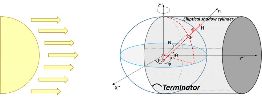
Earth 2021, 2 192
to separate day and night conditions at different ionospheric layers. On this basis, in fact, it
is possible to predict the layer D disappearance during the night or the elevation changes
of the F2 layer peak. Similarly, the knowledge of ST movements is fundamental for the
interpretation of the differential illumination of lower ionospheric layers that can oscillate
following the regular alternation of day and night while, in certain conditions (e.g., at high
latitudes), the upper layers remain always irradiated.
Despite its multi-disciplinary importance, a detailed model for the determination of ST
vertical movements is still lacking. In the scientific literature available to date, manuscripts
dealing with the subject [12] provide only partial solution equations.
In this paper, a Solar Terminator Height (STH) model is proposed which provides,
with unprecedented accuracy and at the global scale, the vertical variation of the ST as a
function of time.
The model also offers methodological support and solution equations to go beyond a
series of approximations (e.g., use of the spherical shape of the Earth, not precise Earth–Sun
position, use of sidereal time, use of the mean terrestrial radius, etc.) still used in all field of
applications, even when greater accuracy would improve the performances.
As an example of the impact of ST variations on space–time dynamics of atmospheric
parameters, the case of ionospheric Total Electron Content (TEC) is particularly addressed.
The TEC represents the number of electrons present along a ray path of 1 m2 of an
ionospheric section, measured in TEC Unit (1 TEC Unit = 1016 electrons/m2 ), and can be
determined by ground-based (e.g., from ionosondes, Global Navigation Satellite Systems
receivers [13]) and space-based (e.g., FORMOSAT/COSMIC series [14,15], DEMETER [16])
measurements.
In this work, a statistically-based analysis of 20 years of GPS (Global Positioning
System)-TEC data measured over Central Italy during the period 2000–2019 is performed
in order to recognize its dependence on STH space–time variations.
The analysis here implemented investigates, for the first time, the correlations between
TEC measurements and STH. In the post-sunset hours, in fact, the sudden variation in
solar irradiation incident on the various ionospheric layers generates variation in total
ionization. Such a study can be particularly useful in the elaboration of ionospheric TEC
models as well as in those applications requiring predicting the behavior of TEC parameter
in specific conditions.
Moreover, due to the fact that the ionosphere directly influences trans-ionospheric
radio waves propagating from satellites to GNSS receivers [17,18], such models are of
vital importance in order to evaluate and correct errors (that can be quite significant) in
GNSS-positioning due to TEC ionospheric irregularities. No less important is the role that
TEC models play in the study of the possible relations between ionospheric perturbations
and seismic activity, theorized by several authors in recent years [19–23].
2. Materials and Methods
This section is divided into two subsections. In the first one, we illustrate the proposed
time-dependent STH model describing how the atmospheric solar illumination varies
during the night along the vertical at a given geographical position. In the second, we report
the method used for the statistical correlation analysis between STH and the ionospheric
TEC parameter measured over Central Italy.
2.1. Solar Terminator Height Determination
The Solar Terminator Height (STH) at time t, h (θ, ϕ, t) for a given point P, at lati-
tude θ and longitude ϕ on the Earth’s surface, represents the height of the Sun-shadow
demarcation line (solar terminator) at the instant t along the vertical at point P (θ, ϕ).
The only assumptions we make in the mathematical modelling are: solar rays parallel
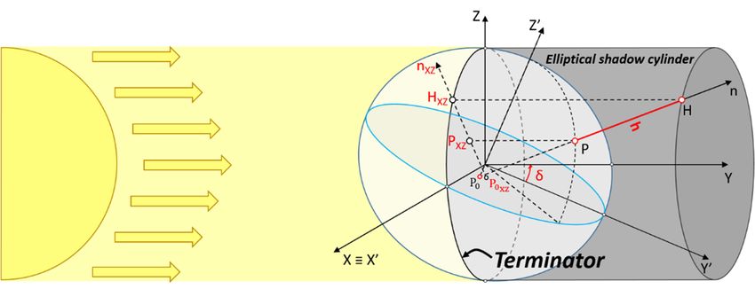
to each other and ellipsoidal (WGS84) shape of the Earth.
The vertical height of the point P above the Earth’s surface is a line joining the point P
and a point H along the local ellipsoid’s normal n (Figure 1). The length PH is called the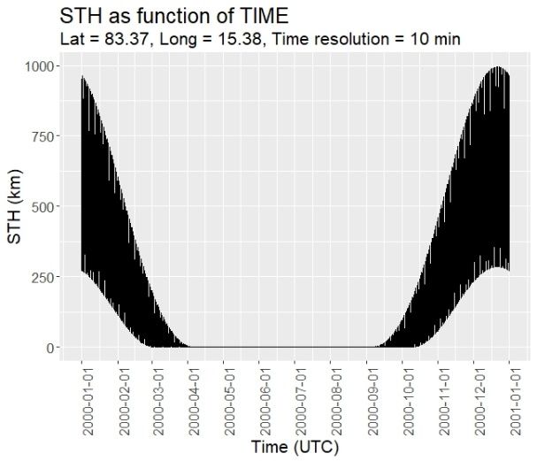
to each other and ellipsoidal (WGS84) shape of the Earth.
The vertical height of the point P above the Earth’s surface is a line joining the point
P and a point H along the local ellipsoid’s normal n (Figure 1). The length is called
the ellipsoidal height h. The ellipsoid’s normal n is a straight line perpendicular to the
Earth 2021, 2 plane tangent to the ellipsoid at the point P and which, then, crosses in a generic point P0 193
the axis of rotation of the Earth.
Therefore, the terminal point H (θ, φ, t) of the solar terminator ellipsoidal height h (θ,
φ, t) is given by the intersection
ellipsoidal between
height h. n and thenormal
The ellipsoid’s boundary
n is aofstraight
the shape
linegenerated by to the plane
perpendicular
the shadow produced by the Earth’s ellipsoid illuminated by the Sun’s rays (elliptical
tangent to the ellipsoid at the point P and which, then, crosses in a generic point P0 the axis
shadow cylinder shown inofFigure
of rotation 1).
the Earth.
Figure 1. Solar illumination
Figure model of the
1. Solar illumination Earth’s
model ellipsoid
of the Earth’satellipsoid
the time at
of the
the time
equinox and
of the representation
equinox of the ellipsoidal
and represen-
tation
height of the solarofterminator
the ellipsoidal
(Solarheight of the Height)
Terminator solar terminator (Solarof
h and of some Terminator
the relatedHeight) h and of some of
parameters.
the related parameters.
Therefore, the terminal point H (θ, ϕ, t) of the solar terminator ellipsoidal height h (θ,
By choosingϕ, t) is given
WGS84 as by the intersection
reference ellipsoidbetween n and theaboundary
and by choosing Cartesianof the shape
reference generated by the
sys-
tem, which for shadow
convenienceproduced
we callbyX”Y”Z”,
the Earth’s ellipsoid
having the Z”illuminated by the
axis coinciding Sun’s
with therays (elliptical shadow
Earth’s
cylinder
rotation axis, the showncoinciding
X”Y” plane in Figure 1).with the equatorial plane and the X” axis which
intersects the primeBy choosing
meridian WGS84
on the as reference
positive side (Figureellipsoid
1), it is and by choosing
possible a Cartesian
to determine the reference
system, which for convenience we call X”Y”Z”, having the
ellipsoidal height h by making it explicit from any of the well-known conversion formulas Z” axis coinciding with the
Earth’s
provided by geodesy: rotation axis, the X”Y” plane coinciding with the equatorial plane and the X”
axis which intersects the prime meridian on the positive side (Figure 1), it is possible
= ( + height
to determine the ellipsoidal ℎ) ∙ cosh by
∙ cos
making; it explicit from any of(1)the well-known
conversion formulas provided by geodesy:
= ( + ℎ) ∙ cos ∙ sin ; (2)
X 00 H = ( N + h)· cos θ · cos ϕ; (1)
= [ ∙ (1 − 00 ) + ℎ] ∙ sin ; (3)
Y H = ( N + h)· cos θ · sin ϕ; (2)
where:
h i
Z 00 H = N · 1 − e2 + h · sin θ; (3)
H is the terminal point of the ellipsoidal height h;
= where:is the length of the straight line coinciding with the ellipsoid’s normal
∙
• the
n connecting H point
is thePterminal
and the point
point of the ellipsoidal
of intersection heightnh;and Z” axis P0 (length
between
a
• N
in Figure 1); = √ is the length of the straight line coinciding with the ellipsoid’s normal
1−e2 ·sin2 θ
n connecting
e2 and a, respectively equal the point P andand
to 0.00669438 the to
point of intersection
6,378,137 between
m, are the n andpa-
ellipsoidal Z” axis P0 (length
PP0 in Figure
rameters first eccentricity 1); and semi-major axis of the reference ellipsoid used
squared
(WGS84); • e2 and a, respectively equal to 0.00669438 and to 6,378,137 m, are the ellipsoidal
parametersthe
θ and φ are, respectively, firstgeodetic
eccentricity squared
latitude and
and the semi-major axis of the reference ellipsoid
longitude.
used (WGS84);
Since we are interested in determining the variation of h as a function of time (and
• θ and ϕ are, respectively, the geodetic latitude and the longitude.
therefore of the angle of rotation of the Earth around its axis), for our purposes it is more
convenient to choose Since
a newweX’Y’Z’
are interested
referenceinsystem,
determining thethe
rotating variation h as a around
X”Y”Z”ofsystem function of time (and
therefore of the angle of rotation of the Earth around its axis), for our purposes it is more
convenient to choose a new X0 Y0 Z0 reference system, rotating the X”Y”Z” system around
the Z” axis, so that, as the Earth rotates, our reference system rotates in the opposite
direction, making sure that the positive side of the X0 axis always passes through the point
of intersection between sunset line and equatorial plane (Figure 1 shows the moment of
the day in which X0 Y0 Z0 coincides with X”Y”Z”).
In order for the proposed equations, (1), (2) and (3), to be valid in the new X0 Y0 Z0
reference system, we replace the longitude ϕ with the angle measured on the equatorial
plane between the meridian passing through the X0 axis (sunset line) and the meridian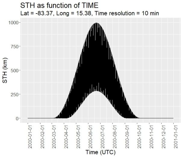
the Z” axis, so that, as the Earth rotates, our reference system rotates in the opposite di-
rection, making sure that the positive side of the X’ axis always passes through the point
of intersection between sunset line and equatorial plane (Figure 1 shows the moment of
the day in which X’Y’Z’ coincides with X”Y”Z”).
In order for the proposed equations, (1), (2) and (3), to be valid in the new X’Y’Z’
Earth 2021, 2 194
reference system, we replace the longitude φ with the angle measured on the equatorial
plane between the meridian passing through the X’ axis (sunset line) and the meridian
passing through the point P. We call this angle λ, local hour angle from sunset. λ, which
varies according to thethrough
passing Earth’s the
rotation,
point will subsequently
P. We call this anglebe accurately determined.
λ, local hour angle from sunset. λ, which
In the new reference system X’Y’Z’, we have:
varies according to the Earth’s rotation, will subsequently be accurately determined.
0 Y0 Z0 , we have:
In the new reference + ℎ) X
= (system ∙ cos ∙ cos ; (4)
X 0 H = ( N + h)· cos θ · cos λ; (4)
= ( + ℎ) ∙ cos ∙ sin ; (5)
Y 0 H = ( N + h)· cos θ · sin λ; (5)
= [ ∙ (1 0− )h+ ℎ] ∙ sin 2 ; i
(6)
Z H = N · 1 − e + h · sin θ; (6)
with λ = local hour angle from sunset.
with λ = local hour angle from sunset.
Furthermore, due to the revolution motion of the Earth around the Sun, the equato-
Furthermore, due to the revolution motion of the Earth around the Sun, the equatorial
rial plane tilts with respect to the direction of the Sun’s rays by an angle δ (solar declination).
plane tilts with respect to the direction of the Sun’s rays by an angle δ (solar declination). δ
δ reaches a maximum
reaches aangle in June
maximum at the
angle inmoment of the
June at the Northern
moment Hemisphere
of the summer
Northern Hemisphere summer
solstice, which is about
solstice, 23.44°,
which is and
abouta minimum
23.44◦ , andangle in December
a minimum angleat in
theDecember
moment of at the
the moment of
Northern Hemisphere
the Northernwinter solstice, which
Hemisphere winteris about −23.44°.
solstice, whichSince the X’−axis
is about 23.44is◦ .perpen-
Since the X0 axis is
dicular to theperpendicular
direction of thetoSun’s rays, the rotation of the angle δ takes place around
the direction of the Sun’s rays, the rotation of the angle theδ takes place
X’ axis itself. Thus, we define
0 a new reference system XYZ obtained by rotating the X’Y’Z’
around the X axis itself. Thus, we define a new reference system XYZ obtained by rotating
reference systemthe Xby
0 Y0the angle -δ system
Z0 reference around by thethe
X’angle
axis (see Figurethe
-δ around 2).XThe angle
0 axis (see δFigure
will be
2). The angle δ
calculated later.
will be calculated later.
Figure
Figure 2. Solar 2. Solar illumination
illumination model of themodel of ellipsoid
Earth’s the Earth’satellipsoid
the time at
ofthe
thetime of the Hemisphere
Northern Northern Hemisphere
winter solstice and
winter
representation of thesolstice andheight
ellipsoidal representation of the
of the solar ellipsoidal
terminator height
(Solar of the solar
Terminator terminator
Height) h, of the(Solar Termina-
declination angle δ and of
tor Height) h, of
some of the related parameters. the declination angle δ and of some of the related parameters.
In the XYZ system, we have:
In the XYZ system, we have:
= = (X +=ℎ)X∙0 cos ∙ cos ; (7)
H H = ( N + h )· cos θ · cos λ; (7)
= ∙ cos −YH =∙ sin = δ − Z 0 · sin δ =
0 · cos
YH H (8) (8)
= ( + ℎ) ∙ cos ∙=sin
( N ∙+cos [ (1
− θ · sin )
∙ λ−· cos δ+−ℎ] N
∙ sin
· 1 −∙ sin
e2 +; h · sin θ · sin δ;
h)· cos
= ∙ sin −ZH =∙ cos YH = δ − Z 0 · cos δ =
0 · sin
H (9) (9)
= ( + ℎ) ∙ cos ∙=sin
( N ∙+sin − [θ · ∙sin
(1 λ−· sin)δ+−ℎ] N
∙ sin e2 +. h · sin θ · cos δ.
· 1 −∙ cos
h)· cos
Solving Equation (7) for
Solving h gives:
Equation (7) for h gives:
XH
h= − N; i f : α ≤ 0◦ (10)
cos θ · cos λ
where α = solar elevation angle, to be defined later.
Therefore, we need to calculate XH to determine h. To do this, it is possible to exploit
the fact that (given the assumption of solar rays all parallel to each other) the projection on
the XZ plane of the point H is a point Hxz given by the intersection between the projection
on the XZ plane of n (nxz ) and the ellipsoid E (see Figure 2). It will, then, be necessary to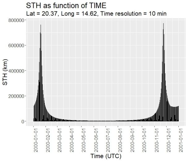
Earth 2021, 2                                                                                            195

                determine the equation of the two geometric figures (n and E) and their intersection at the
                point Hxz .
                     nxz is a straight line passing through the projections on the XZ plane of the points P
                and P0 . The coordinates of the points P and P0 in the X”Y”Z” reference system are given,
                again, by the well-known equations of the ellipsoid’s normal provided by geodesy:

                                                   X 00 P = N · cos θ · cos ϕ;                          (11)

                                                  Y 00 P = N · cos θ · sin ϕ;                           (12)

                                                 Z 00 P = N · 1 − e2 · sin θ;                           (13)
                                                             00
                                                            XP0 = 0;                                    (14)
                                                             00
                                                            YP0 = 0;                                    (15)
                                                      00
                                                     ZP0 = −e2 · N · sin θ.                             (16)
                     Applying the equations of rotation already used to rotate the point H from the refer-
                ence system X”Y”Z” to the reference system XYZ, the points P and P0 in XYZ are given by
                the following expressions:
                                                     XP = N · cos θ · cos λ;                         (17)

                                   ZP = N · cos θ · sin λ· sin δ + N · 1 − e2 · sin θ · cos δ;       (18)

                                                            XP0 = 0;                                    (19)

                                                 ZP0 = −e2 · N · sin θ · cos δ.                         (20)
                     At this point, we can determine the equation of the line nxz passing through the points
                P e P0 (and through the point Hxz ; see Figure 2):

                                                  Xn − XP0   Zn − ZP0
                                                           =          ;                                 (21)
                                                  XP − XP0   ZP − ZP0

                                                            Zn − ZP0
                                                     Xn =            · XP .                             (22)
                                                            ZP − ZP0
                     From the Equations (17), (18) and (20), after some simplifications, we have:

                                              XP                 cos λ
                                                    =                              ;                    (23)
                                           ZP − ZP0   sin λ· sin δ + tan θ · cos δ

                defining:
                                                                cos λ
                                              C1 =                                ;                     (24)
                                                     sin λ· sin δ + tan θ · cos δ
                we can write:
                                                   Xn = Zn − ZP0 ·C1 .                                  (25)
                     Let’s now move on to the equation of the ellipsoid E, which, in the X”Y”Z” reference
                system, coincides with the one in the X0 Y0 Z0 reference system:

                                                 X0 E 2 + Y0 E 2  Z0 2
                                                          2
                                                                 + 2E = 1;                              (26)
                                                        a          c
                where c, equal to 6,356,752.314 m, is the semi-minor ellipsoid parameter of the reference
                ellipsoid used (WGS84).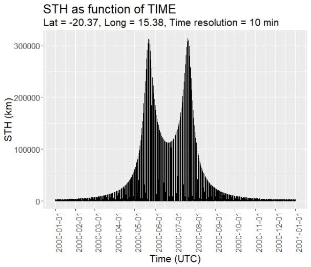
Earth 2021, 2                                                                                              196

                     We determine the equation of the coordinate XE as a function of ZE on the XZ plane
                (for Y = 0). Again exploiting the rotation equations of the reference system, in XYZ, after
                some substitutions, we have:
                                                         XE0 = XE ;                                    (27)
                                                                  sin δ
                                                    YE0 = ZE0 ·         = ZE0 · tan δ;                    (28)
                                                                  cos δ
                                      ZE − YE0 · sin δ   ZE − ZE0 · tan δ· sin δ   Z
                              ZE0 =                    =                         = E − ZE0 · tan2 δ;      (29)
                                          cos δ                  cos δ            cos δ
                from which:
                                                                      ZE
                                                      ZE0 =                     ;                        (30)
                                                              cos δ· 1 + tan2 δ
                                                                   ZE · tan δ
                                                      YE0 =                     .                        (31)
                                                              cos δ· 1 + tan2 δ
                     By replacing Equations (27), (31) and (30) in (26), we have:
                                                               2                        2
                                 XE2           ZE · tan δ

                                                                              ZE
                                     +                           +                           = 1;         (32)
                                 a2      a· cos δ·(1 + tan2 δ)      c· cos δ·(1 + tan2 δ)
                                                                 2                            2
                                 XE2             ZE · tan δ

                                                                                    ZE
                                     +                              +                              = 1;   (33)
                                 a2       a· cos δ·(1 + tan2 δ)         c· cos δ·(1 + tan2 δ)
                                      XE2                                     tan2 δ

                                                2             1                          1
                                           + ZE ·                     2 ·           + 2 = 1;            (34)
                                      a2            cos δ·(1 + tan2 δ)           a2      c

                                                                                             a2

                                       2       2      2            1                   2
                                     X E = a − ZE ·                          2 · tan δ + 2 .            (35)
                                                          cos δ·(1 + tan2 δ)                 c

                     Defining:
                                                                                       a2

                                                              1                  2
                                           C2 =                       2 ·   tan  δ +      ;             (36)
                                                    cos δ·(1 + tan2 δ)                 c2

                we can write:
                                                          XE2 = a2 − ZE2 ·C2 ;                            (37)
                and, squaring the Equation (25), we obtain:

                                        Xn2 = Zn2 ·C12 − Zn · 2· ZP0 ·C12 + ZP20 ·C12 .                   (38)

                     Thus, given the expressions of Xn (Zn ) and XE (ZE ), (38) and (37), it is possible to
                determine their point of intersection ZH (XH ) by equating them:

                                  Z2H · C12 + C2 − ZH · 2· ZP0 ·C12 + ZP20 ·C12 − a2 = 0.              (39)

                     Defining:
                                                            K1 = C12 + C2 ;                               (40)
                                                           K2 =     2· ZP0 ·C12 ;                         (41)

                                                          K3 = ZP20 ·C12 − a2 ;                           (42)
                we can write:                                       q
                                                           K2 ±         K22 − 4·K1 ·K3
                                                    ZH =                                 .                (43)
                                                                        2K1
                     We use the positive sign if θ + δ > 0 and the negative sign if θ + δ < 0.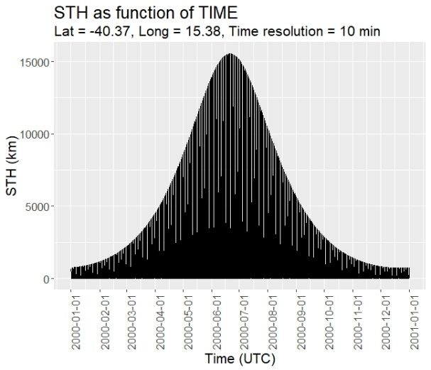
Earth 2021, 2                                                                                            197

                     From Equation (25), it follows that:

                                                    X H = ZH − ZP0 ·C1 ;                                (44)

                and, finally, it is possible to compute the Equation (10):

                                                        XH
                                      h = STH =                   − N.       i f : α ≤ 0◦               (45)
                                                    cos θ · cos λ
                     The last step consists in determining the three unknown angles:
                •    Solar declination angle δ;
                •    Local hour angle from sunset λ;
                •    Solar elevation angle α.
                      We use the equations proposed in Chapters 25, 7, 22 and 30 of the book Astronomical
                Algorithms [24] for the accurate determination of the solar declination angle δ and the equa-
                tions proposed in Chapters 28, 22 and 25 of the same book [24] for the determination of
                the equation of time ET, as a function of which the angles λ and α will then be determined.
                The proposed equations can also be deduced from the spreadsheets available online on the
                NOAA solar calculator website [25], also based on the book Astronomical Algorithms [24].
                However, given that the equations proposed by [24] have different scopes from those pro-
                posed in the present work and different possibilities of choosing the “previous parameters”
                according to the use of the “dependent parameters” and that over time there have been
                some updates to the equations, it is preferred to reorganize them and report them below
                for clarity and simplicity of use.

                2.1.1. Solar Declination Angle: δ
                     The equations proposed in Chapters 25, 7, 22 and 30 of [24] for the accurate determi-
                nation of the solar declination angle δ are then reorganized below.
                     Defining JD as the Julian Day from the epoch “1 January 2000 12:00:00 UTC”, it is
                possible to determine the time T expressed in Julian centuries:

                                                                JD
                                                         T=          ;                                  (46)
                                                               36525
                     It is considered superfluous to report the JD calculation procedure as nowadays
                any programming language has at least one function for its calculation; in any case, the
                procedure can be found in Chapter 7 of [24].
                     Thus, the Sun’s Mean Longitude (ML), referring to the mean equinox of the date
                (decimal degrees), is:

                                   ML = 280.46646◦ + T(36000.76983◦ + 0.0003032◦ ·T);                   (47)

                where 280.46646◦ is the mean longitude of the Sun on 1 January 2000 at noon UTC (mean
                equinox of the date).
                    Then, the Sun’s Mean Anomaly MA is given by:

                                   MA = 357.52911◦ + T(35999.05029◦ − 0.0001537◦ ·T);                   (48)

                      MA is defined as “the angular distance from perihelion which the planet would have
                if it moved around the Sun with a constant angular velocity” [24] (Cap. 30, p. 194).
                      As a function of MA, it is now possible to calculate the Sun’s equation of the center
                C, that is, the angular difference between the actual position of a body in its elliptical
                orbit and the position it would occupy if its motion were uniform in a circular orbit of the
                same period.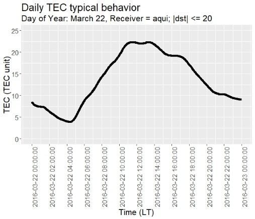
Earth 2021, 2                                                                                                198

                     C can be performed as follows:

                            C = sin( MA)·(1.914602◦ − T (0.004817◦ + 0.000014◦ · T )) + sin(2T )
                                                                                                           (49)
                                     ·(0.019993◦ − 0.000101◦ · T ) + sin(3T )·0.000289◦ ;

                By adding Sun’s equation of the center C to Sun’s Mean Anomaly MA, we calculate the Sun’s
                true longitude TL (the true geometric longitude referred to the mean equinox of the date):

                                                        TL = ML + C;                                       (50)

                      The Sun’s Apparent longitude AL, i.e., TL corrected for the nutation and the aberration,
                is given by:

                               AL = TL − 0.00569◦ − 0.00478◦ · sin(125.04◦ − 1934.136◦ · T );              (51)

                     The next step is to calculate the mean obliquity of the ecliptic MOE. The equation
                proposed by the 1998 version of Astronomical Algorithms [24], which we are using as the
                main reference, shows terms up to the third order. This equation is still in use also in
                the spreadsheets available online on the NOAA solar calculator website [25], but the JPL’s
                fundamental ephemerides are constantly updated. In particular, the MOE calculation was
                updated in the Astronomical Almanac for the year 2010 [26], which, in addition to correcting the
                coefficients for the terms up to the third order, adds the terms of the fourth and fifth orders:

                         MOE = 23◦ 260 2100 , 406 − 4600 , 836769T − 000 , 0001831T 2 +000 , 00200340T 3
                                                                                                           (52)
                                             −000 , 576·10−6 T 4 − 400 , 34·10−8 T 5 ;

                where, again, T is the time measured in Julian centuries from noon 1 January 2000 UTC.
                    Once MOE is known, it is possible to compute the obliquity corrected OC, which
                should be considered in order to calculate the apparent position of the Sun (position of the
                Sun corrected for the nutation and the aberration):

                                    OC = MOE + 0.00256◦ · cos(125.04◦ − 1934.136◦ · T );                   (53)

                     Finally, the Sun’s declination δ is given by:

                                                  δ = asin(sin OC · sin AL);                               (54)

                2.1.2. Equation of Time: ET (min)
                     For the precise determination of the angles λ and α, instead, we use the equation of
                time ET, the calculation of which is proposed in Chapter 28 (with references to Chapters 22
                and 25) of the book Astronomical Algorithms [24].
                     ET is a corrective parameter of the heliocentric longitude of the Earth and therefore of
                solar time. In particular, it transforms the mean solar time MST into the true solar time TST.
                     MST, in fact, is calculated on the basis of the assumption of Earth’s constant velocity
                of revolution along a circular orbit, rather than an elliptical one. Furthermore, at a much
                lower magnitude, the equation of time also corrects the variations in the Earth’s speed
                along the elliptical due to the interaction with the Moon and with the planets.
                     ET expressed in minutes is given by the following expression:

                         ET = [y· sin(2· ML) − 2·e· sin( MA) + 4·e·y· sin( MA)· cos(2· ML) − 1/2
                                                                                   min                     (55)
                                      ·y2 · sin(4· ML) − 5/4e2 · sin(2· MA) · 1440

                                                                                360◦ ;

                where e = eccentricity of the Earth’s orbit:

                                   e = 0.016708634 − 0.000042037· T − 0.0000001267· T 2 ;                  (56)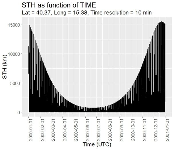
Earth 2021, 2                                                                                                 199

                     y = coefficient of correction of the position of the Sun for the nutation and the aberration:

                                                                    OC
                                                         y = tan2      ;                                     (57)
                                                                     2

                2.1.3. Local Hour Angle from Sunset λ
                     The angle λ is defined as the local hour angle from sunset since it represents the local
                hour angle LHA reduced by 90◦ . In fact, LHA, which is the angle between the meridian
                passing through the geographical position of the Sun and the meridian passing through
                the geographical position of the point P, measures 0◦ when the point P is at solar noon.
                Similarly, λ is equal to 0 when the meridian passing through the point P coincides with the
                meridian passing through the point where sunset occurs on the equatorial plane.
                     For its determination, the following 4 steps are carried out:
                1.   HD (min/UTC), the hour of the day hh:mm:ss UTC of point P expressed in minutes,
                     is calculated:

                                                 HD = hh·60 + mm + ss/60;                                    (58)
                2.   TST (min/UTC), the true solar time of point P expressed in minutes, is obtained
                     as follows:

                                          TST = ( HD + ET + 4· ϕ) mod 1440 min;                              (59)
                3.   LHA (◦ ), the local hour angle of point P expressed in degrees, is given by:

                                                    LH A = TST/4 − 180◦ ;                                    (60)
                4.   λ (◦ ), local hour angle from sunset expressed in degrees, then, is:

                                                 λ = ( LH A − 90◦ ) mod 360◦ ;                               (61)

                2.1.4. Solar Elevation Angle α
                      Finally, still exploiting the knowledge of the LHA, it is possible to calculate α (◦ ), the
                solar elevation angle, expressed in degrees:

                                        α = asin(sin θ · sin δ + cos θ · cos δ· cos LH A).                   (62)

                     A computer code for the time-dependent STH calculation for any geographic location
                on the globe was written using the R programming language [27]. This code can be found
                in the Supplementary Materials (Supplementary 1) to this paper.

                2.2. STH–TEC Correlation Analysis
                      A simple look at the typical behavior of TEC measurements clearly enhances their
                strict dependence on the daily solar variation (see Figure 3, [28]).
                      Solar forcing also causes seasonal variations [29–31]; however, it is not the unique
                cause of ionospheric TEC deviations. For instance, geomagnetic activity (and storms) can
                significantly affect TEC so that, in order to discriminate solar from other contributions, it is
                particularly important to study those parts of the day (before sunrise or after sunset) when
                ionospheric layers are selectively illuminated by the Sun [32] (Figure 3).
                      In order to evaluate solar contribution to TEC variations (as a function of the specific
                location and time of year and in different conditions of solar activity), a correlation analysis
                with STH after sunset was performed. A simple linear regression model and a log-linear
                regression model, accompanied by the estimate of Pearson’s linear correlation coefficient,
                were used to verify the existence of a relationship between the two variables and the
                relative degree of correlation between them.
Earth 2021, 2 200
In the data preprocessing phase, the following data selection and filtering operations
Earth 2021, 2, FOR PEER REVIEW were implemented in order to respond to the double need for homogeneity and 10 statistical
significance of the TEC data under investigation.
Figure 3.
Figure 3.TEC
TECmeasurements
measurements collected by the
collected byGPS
the L’Aquila receiverreceiver
GPS L’Aquila (Central(Central
Italy) on Italy)
22 March
on 22 March 2016
2016 showing the fairly standard behavior of TEC at mid-latitudes (in quiet geomagnetic activity
showing the
conditions). fairly standard behavior of TEC at mid-latitudes (in quiet geomagnetic activity conditions).
Collection of TEC Data Samples
Solar forcing also causes seasonal variations [29–31]; however, it is not the unique
causeThe analyzed Total
of ionospheric Electron Content
TEC deviations. For instance,(TEC) data wereactivity
geomagnetic obtained
(andusing the
storms) open-source
can
software
significantlyIONOLAB-TEC
affect TEC so that,[33];
in this
ordersoftware, developed
to discriminate by the
solar from Ionospheric
other Research
contributions, it Labo-
is particularly
ratory important toUniversity
of the Hacettepe study those of parts of the (Turkey),
Ankara day (beforeelaborates
sunrise or after sunset) TEC (slant
the vertical
whencalculated
TEC ionospheric layersthe
along arejoining
selectively
GPS illuminated
satellite–GPSby thereceiver
Sun [32]corrected
(Figure 3).for vertical direction)
In order to evaluate solar contribution to TEC variations (as a function of the specific
using the method described in [34] and offers the possibility to test its effectiveness by
location and time of year and in different conditions of solar activity), a correlation anal-
comparison with TEC estimates from IGS analysis centers. The satellite DCB (Differential
ysis with STH after sunset was performed. A simple linear regression model and a log-
Code Bias) is obtained
linear regression from IONEX
model, accompanied by thefiles, and the
estimate receiverlinear
of Pearson’s DCBcorrelation
is obtainedco- using the
IONOLAB-BIAS
efficient, were usedalgorithm detailed
to verify the existenceinof[35]. The temporal
a relationship resolution
between of the TEC
the two variables anddata is 30 s.
To avoid
the relative comparing
degree non-homogeneous
of correlation between them. data, we proceeded, first of all, to sample only
data In coming
the datafrom the samephase,
preprocessing GPS the
receiver,
following and then
data measured
selection in theoperations
and filtering same geographical
were implemented
position. The one in order to
located inrespond
CentraltoItaly
the double needof
in the city forL’Aquila
homogeneity
was and statistical
chosen as the reference
significance
station of the TEC data
for estimating theunder
TEC,investigation.
whose GPS receiver is called AQUI (Lat.: 42.368, Long.:
13.35). We chose this station as it is the one that provides the longest historical series of data
Collection of TEC Data Samples
at national level, lasting over 20 years. We then analyzed the twenty-year time interval that
The analyzed Total Electron Content (TEC) data were obtained using the open-source
goes from 1 January 2000 00:00:00 to 1 January 2020 00:00:00 of TEC data.
software IONOLAB-TEC [33]; this software, developed by the Ionospheric Research La-
As aoffirst
boratory operation,
the Hacettepe in orderofto
University avoid(Turkey),
Ankara unnecessary delays
elaborates in processing
the vertical TEC (slantthe twenty-
year time series under analysis, the data were downsampled from
TEC calculated along the joining GPS satellite–GPS receiver corrected for vertical 30 s to 10 min. The time
direc-
interval
tion) usingof the
30 smethod
between successive
described in [34]observations
and offers thewas, in fact,
possibility to considered the low temporal
test its effectiveness
dynamic of thewith
by comparison signal,
TECconsidered excessively
estimates from short
IGS analysis for the
centers. Thepurposes
satellite DCBof this work.
(Differ-
entialThe
Code Bias)
next stepis obtained from IONEX
of pre-processing thefiles,
data,and the receiver DCB
implemented is obtained
in order using
to prepare them for the
the IONOLAB-BIAS
linear correlation studyalgorithm
withdetailed
the STH in variable,
[35]. The temporal resolution
was to filter the TEC of the TECsaving
data, data only the
is 30 s.
data recorded at the times of our interest, that is, from the time of sunset to solar midnight
at the geographical position of the AQUI-GPS receiver.
The TEC, as previously anticipated, is a parameter that varies not just in response to
the normal daily/seasonal solar cycle but also according to additional known and unknown
sources. Known further sources of variation are intensification of solar activity as wellEarth 2021, 2 201
as the already mentioned geomagnetic activity both affecting TEC above the geographic
location under observation.
Therefore, a twenty-year dataset of observations was built, including the measured
indices of solar activity F10.7 and of geomagnetic activity (Dst) obtained from NASA’s data
supply service [36]. Using the 20:00 measurement of the F10.7 index and the hourly mea-
surements of the Dst index, for each of the two parameters, through a linear interpolation
operation between successive values, the difference in time resolution with the TEC index
(which is equal to 10 min) was filled. Both are indices measured on a global scale, which,
however, influence the TEC parameter to a variable extent, even at a local level.
In particular, geomagnetic activity is more difficult to manage, as it can generate
anomalous and unpredictable local variations in the electron content in the ionosphere.
Therefore, to determine to what extent the TEC may vary as a function just of the portion
of the ionosphere illuminated by the Sun, periods affected by intense (|Dst| > 20 nT)
geomagnetic activity were excluded by the dataset.
In order to take into account TEC dependence on both seasonal solar cycle and active-
Sun periods, the twenty-year dataset was divided into 12 monthly groups, one for each
month of the year, and into 6 groups according to the parameter F10.7 (6 ranges of solar
activity shown in Table 1) in order to obtain 72 homogeneous datasets.
Table 1. Solar activity levels of F10.7 index in solar flux unit (s.f.u.) in which the STH–TEC linear
regression graphs are grouped.
Solar Activity Level Range 1 Range 2 Range 3 Range 4 Range 5 Range 6
F10.7 (s.f.u.) 0–80 80–100 100–120 120–140 140–160 160–Inf.
3. Results
3.1. STH as Function of Time
Figures 4–6 give some examples of time-dependent STH values computed following
the model described in Section 2.1 over three pairs of points chosen in both hemispheres
Earth 2021, 2, FOR PEER REVIEW 12
in three different (Tropical, Temperate and Polar) Zones. The temporal resolution of the
graphs is 10 min, and the STH values are shown for an entire year (2000).
(a) (b)
Figure 4.
Figure 4. Examples of time-dependent STH determination by using the proposed model. The two figures show the trend trend
of STH
of STH asas aa function
function of
of time
time over
over an
an entire
entire year
year (2000)
(2000) in
in tropical
tropical latitudes.
latitudes. Figure
Figure (a)(a) represents
represents STH
STH in
in the
the Northern
Northern
Hemisphere. Figure
Hemisphere. Figure (b)
(b) represents
represents STH
STHininthe
theSouthern
SouthernHemisphere.
Hemisphere.Note Notethat,
that,ininthe two
the twoSTH
STHpeaks—corresponding
peaks—corresponding to
the solar midnight of the two days of the year in which the latitude θ is closest to −δ (declination)—small variations in
to the solar midnight of the two days of the year in which the latitude θ is closest to −δ (declination)—small variations
computation time or longitude are enough to ensure that each of the two STH peaks varies considerably (in fact, if it were
in computation time or longitude are enough to ensure that each of the two STH peaks varies considerably (in fact, if it
θ = −δ, when SZA = −180, it would be STH = ∞). Therefore, precise longitude values were chosen, such as to better empha-
were θ = −an
size such when SZA = −180, it would be STH = ∞). Therefore, precise longitude values were chosen, such as to better
δ, aspect.
emphasize such an aspect.(a) (b)
Figure 4. Examples of time-dependent STH determination by using the proposed model. The two figures show the trend
of STH as a function of time over an entire year (2000) in tropical latitudes. Figure (a) represents STH in the Northern
Hemisphere.
Earth 2021, 2 Figure (b) represents STH in the Southern Hemisphere. Note that, in the two STH peaks—corresponding to 202
the solar midnight of the two days of the year in which the latitude θ is closest to −δ (declination)—small variations in
computation time or longitude are enough to ensure that each of the two STH peaks varies considerably (in fact, if it were
θ = −δ, when SZA = −180, it would be STH = ∞). Therefore, precise longitude values were chosen, such as to better empha-
size such an aspect.
(a) (b)
Figure 5.
Figure 5. Examples
Examples of
of time-dependent
time-dependent STH
STH determination
determination by
by using
using the
the proposed
proposed model.
model. The
The two
two figures
figures show
show the
the trend
trend
Earth 2021, 2, FOR PEER REVIEW 13
of STH
of STH as
as aa function
function of
of time
time over
over an
an entire
entire year
year (2000)
(2000) in
in temperate
temperate latitudes.
latitudes. Figure
Figure (a)
(a) represents
represents STH
STH in
in the
the Northern
Northern
Hemisphere. Figure (b) represents STH in the Southern Hemisphere.
Hemisphere. Figure (b) represents STH in the Southern Hemisphere.
Northern Southern Southern
polar night Northern polar day polar night
polar day
(a) (b)
Figure 6. Examples of time-dependent
time-dependentSTHSTHdetermination
determinationby byusing
usingthe
theproposed
proposedmodel.
model.The
The
twotwo figures
figures show
show thethe trend
trend of
of STH as a function of time over an entire year (2000) in polar latitudes. Figure (a) represents STH in the Northern Hem-
STH as a function of time over an entire year (2000) in polar latitudes. Figure (a) represents STH in the Northern Hemisphere.
isphere. Figure
Figure (b) (b) represents
represents STH
STH in the in the Southern
Southern Hemisphere.
Hemisphere.
As
As can
can be
be seen,
seen, the graphs proposed
the graphs proposed reflect
reflect expected
expected STH annual
annual behavior.
behavior. In
In the
the
case of the first two plots (Figure 4), relating to intertropical
case of the first two plots (Figure 4), relating to intertropical latitudes, the solar terminator
reaches
reaches peak
peak altitudes
altitudes inin the
the few winter nights in which the vertical to the considered
geographical
geographical position
position isis almost
almost parallel
parallel to
to the
the direction
direction of the Sun’s rays, going to meet
the
the Sun-shadow
Sun-shadow line line at
at hundreds of thousands of kilometers of altitude, before dropping
abruptly.
abruptly. AtAt mid-latitudes
mid-latitudes (Figure
(Figure 5),
5), however,
however, the nocturnal
nocturnal peak heights show more
tenuous
tenuous variations, touching the maximum and minimum values
variations, touching the maximum and minimum values at
at the relative winter
and
and summer
summer solstices.
solstices. Finally,
Finally, at polar latitudes, it is possible to appreciate the alternation
of the months
of months of polar day and polar night, with maximum daily values of STH that are
maintained in the order of hundreds (or a few thousand) of kilometers of altitude.
maintained
3.2. STH–TEC
3.2. STH–TEC Correlation
Correlation Analysis
Analysis
In this section, we showthe
In this section, we show theresults
resultsofofa apreliminary
preliminarystudy onon
study STH–TEC
thethe STH–TEC correlation
correla-
analysis
tion during
analysis the period
during between
the period sunset
between sunsetandand
solar midnight.
solar In In
midnight. particular, thethe
particular, scatter
scat-
ter plots and the regression lines for the two variables were monthly processed in different
conditions of solar activity. As a representative example of how the correlation evolves on
average in the six ranges of solar activity, we show the plots related to the solar activity
level between 100 and 120 s.f.u. (Figure 7). The other five ranges of solar activity plots canEarth 2021, 2 203
plots and the regression lines for the two variables were monthly processed in different
conditions of solar activity. As a representative example of how the correlation evolves on
average in the six ranges of solar activity, we show the plots related to the solar activity
level between 100 and 120 s.f.u. (Figure 7). The other five ranges of solar activity plots
can be found in the Supplementary Materials to this paper (Supplementary). The TEC
data used in the analysis were collected by the AQUI GPS receiver located in Central Italy
(Lat.: 42.37; Long.:13.35). At the top of each graph, the corresponding linear correlation
Earth 2021, 2, FOR PEER REVIEWcoefficient, the root mean squared error (RMSE) and the daily mean Time Coverage14 (TC) of
the month are reported.
Figure 7. The 12 graphs show the TEC–STH scatter plots and the related linear regression line of 20 years (2000–2019) of
Figure 7. The 12 graphs show the TEC–STH scatter plots and the related linear regression line of 20 years (2000–2019) of
data grouped by month, with solar activity level between 100 and 120 s.f.u., under quiet geomagnetic conditions and in
data grouped
the time by month,
interval with solar
between sunsetactivity level
and solar between
midnight. The100 andcorrelation
linear 120 s.f.u., under quiet
coefficient, thegeomagnetic conditions
root mean squared error and
and in the
time interval
the dailybetween
mean Timesunset and solar
Coverage (TC) ofmidnight.
the month The linearat
are shown correlation coefficient,
the top of the graphs. the root mean squared error and the
daily mean Time Coverage (TC) of the month are shown at the top of the graphs.
The statistical analysis carried out on the time interval between sunset and solar mid-
night
Thehighlights,
statisticalasanalysis
expected,carried
a negative
outcorrelation
on the time between STH between
interval and TEC, which,
sunsetalbeit
and solar
to a more
midnight or less marked
highlights, extent, always
as expected, exists. In
a negative other words,
correlation in this period
between STH andof timeTEC,andwhich,
in the
albeit to absence
a more of orhigh
lessgeomagnetic
marked extent, activity, regardless
always exists.of In
theother
solar activity,
words, itincanthisbeperiod
ex- of
timepected
and that, as the
in the portion
absence ofofhigh
the atmosphere
geomagnetic illuminated
activity,byregardless
the sun decreases
of the (increasing
solar activity, it
canSTH), the TEC also decreases.
be expected that, as the portion of the atmosphere illuminated by the sun decreases
From the visual analysis of the monthly scatter plots generated in presence of solar
(increasing STH), the TEC also decreases.
activity between 100 and 120 s.f.u., it is quite evident that, if on the one hand there is a
From the visual analysis of the monthly scatter plots generated in presence of solar
fairly clear TEC–STH linear anti-correlation during the spring–summer period (in partic-
activity between
ular during the100 andMay–August),
period 120 s.f.u., it isonquite
the evident
other, in that, if on the one hand
the autumn–winter period there
the is
de-a fairly
clear TEC–STH linear anti-correlation during the spring–summer
crease in TEC as STH increases is considerably more marked in the first 200–500 km of period (in particular
during the period
altitude, a trend May–August), on the other,
that, probably, during the periodin the autumn–winter period
September–March, the decrease
can be better de- in
TEC as STH increases is considerably more marked in the first
scribed with a log-linear regression (this would imply that the TEC–STH relationship is 200–500 km of altitude, a
trend that, probably, during the period September–March, can be better described with a
exponential).
log-linear Another element
regression thatwould
(this can be imply
seen when
thatlooking at plots individually
the TEC–STH relationshipisisthe tendency
exponential).
of Another
TEC to decrease
element that can be seen when looking at plots individually is thesimilar
(as STH increases) during spring–summer months always at tendency of
rates within
TEC to decrease the(as
same
STH graph (the higher
increases) the TEC
during at sunset, the higher
spring–summer monthsthealways
TEC at midnight).
at similar rates
This, during this period, when the correlation tends to be linear, gives the graphs the prop-
within the same graph (the higher the TEC at sunset, the higher the TEC at midnight). This,
erty of homoscedasticity, a desirable property, as it implies that the errors on TEC do not
during this period, when the correlation tends to be linear, gives the graphs the property of
vary as STH varies. However, this element allows us to assume that the correlation be-
homoscedasticity, a desirable property, as it implies that the errors on TEC do not vary as
tween the two parameters has further margins for improvement if only the causes under-
STH varies.
lying However,
the higher thiselectronic
or lower element content
allows at ussunset
to assume
withinthatthe the correlation
ionospheric layerbetween
could the
twobeparameters
identified. Some has further margins
table checks, forout
carried improvement
on a sample basis,if only thehow
show causes underlying
the initial TEC the
variation is only rarely attributable to slight variations in solar or geomagnetic activity
within the predetermined ranges but often remains unjustified.
Given the exponential trend detected by the graphs during the autumn–winter pe-
riod, a monthly log-linear regression analysis was also performed for each of the six solar
activity ranges. Figure 8 shows, again by way of example, the monthly graphs of the log-Earth 2021, 2 204
higher or lower electronic content at sunset within the ionospheric layer could be identified.
Some table checks, carried out on a sample basis, show how the initial TEC variation is
only rarely attributable to slight variations in solar or geomagnetic activity within the
Earth 2021, 2, FOR PEER REVIEW predetermined ranges but often remains unjustified. 15
Given the exponential trend detected by the graphs during the autumn–winter period,
a monthly log-linear regression analysis was also performed for each of the six solar activity
ranges. Figure 8analysis
linear correlation shows,for again by way
the period of example,inthe
October–March themonthly
same range graphs
of solarofactivity
the log-linear
as in Figure 7analysis
correlation (100 s.f.u. < F10.7
for < 120 s.f.u.).
the period The other log-linear
October–March plots can
in the same be found
range of solarin the
activity as
supplementary
in Figure 7 (100 materials
s.f.u.Earth 2021, 2 205
Table 2. TEC–STH correlation coefficient values for the sunset–solar midnight period obtained in each
of the 12 months of the year in each of the 6 predetermined solar activity ranges and for both linear
(Lin) and log-linear (Log-Lin) correlation. The values in bold are the maximums in the comparison
between Lin and Log-Lin, whose cells are highlighted in yellow and green, respectively.
Linear and Log-Linear TEC–STH Correlation Coefficients Comparison
100 < F10.7 < 120 < F10.7 < 140 < F10.7 <
F10.7 < 80 80 < F10.7 < 100 F10.7 > 160
120 140 160
Month
Log- Log- Log- Log- Log- Log-
Lin Lin Lin Lin Lin Lin
Lin Lin Lin Lin Lin Lin
1 −0.38 −0.45 −0.55 –0.67 –0.48 –0.65 –0.60 –0.78 –0.60 –0.79 –0.45 –0.63
2 –0.45 –0.50 –0.64 –0.68 –0.58 –0.69 –0.71 –0.82 –0.69 –0.81 –0.47 –0.53
3 –0.49 –0.50 –0.66 –0.64 –0.70 –0.74 –0.70 –0.72 –0.71 –0.71 –0.67 –0.66
4 –0.66 –0.56 –0.67 –0.60 –0.66 –0.57 –0.74 –0.69 –0.71 –0.68 –0.59 –0.63
5 –0.66 –0.53 –0.61 –0.49 –0.72 –0.58 –0.78 –0.67 –0.65 –0.56 –0.77 –0.70
6 –0.69 –0.55 –0.60 –0.50 –0.63 –0.52 –0.65 –0.56 –0.72 –0.61 –0.62 –0.52
7 –0.70 –0.58 –0.66 –0.53 –0.77 –0.63 –0.76 –0.62 –0.76 –0.64 –0.63 –0.53
8 –0.64 –0.53 –0.67 –0.57 –0.80 –0.69 –0.79 –0.67 –0.78 –0.65 –0.75 –0.63
9 –0.54 –0.52 –0.65 –0.63 –0.79 –0.78 –0.61 –0.66 –0.75 –0.76 –0.64 –0.65
10 –0.44 –0.42 –0.67 –0.58 –0.66 –0.74 –0.62 –0.73 –0.69 –0.83 –0.59 –0.70
11 –0.42 –0.44 –0.58 –0.60 –0.52 –0.63 –0.59 –0.74 –0.65 –0.82 –0.55 –0.75
12 –0.39 –0.45 –0.47 –0.60 –0.64 –0.78 –0.57 –0.75 –0.62 –0.82 –0.54 –0.76
Table 3. Averages of the TEC–STH correlation coefficients of the periods May–August (linear) and
November–February (log-linear), in each of the 6 predetermined solar activity ranges. The values in
bold are the maximums in the comparison between Lin and Log-Lin, whose cells are highlighted in
yellow and green, respectively.
Seasonal Means of The TEC–STH Correlation Coefficients
80 < F10.7 < 100 < F10.7 120 < F10.7 140 < F10.7
F10.7 < 80 F10.7 > 160
100 < 120 < 140 < 160
Lin
−0.67 −0.64 −0.73 −0.74 −0.73 −0.69
(May–Aug)
Log-Lin
−0.46 −0.64 −0.69 −0.77 −0.81 −0.67
(Nov–Feb)
In the case of linear correlation, there is no particular trend as the solar activity varies,
while in the case of log-linear correlation, as the solar activity increases the correlation
coefficient also increases. The case where F10.7 is greater than 160 s.f.u. is an exception
showing a reduction of the log-linear correlation coefficient likely due to the major weights
assumed by F10.7 outliers compared with a reduced population of records.
4. Discussion
The availability of an accurate solar illumination model of the Earth’s atmosphere
could be functional to the improvement of studies relating to the whole series of applica-
tions (AGW/TID, vertical pressure and temperature profiles, neutral and ionic atmospheric
components, electromagnetic waves, total electron content, ionospheric empirical models,
etc.) already discussed in the introductory section.
The TEC–STH dependence relationships that were determined, on the other hand,
have the ultimate aim of describing and better predicting the nocturnal behavior of the TEC
parameter to obtain useful information for improving the processing of empirical models
and forecasting models. In this sense, also given the absence of previous studies on the
same topic, the investigation initiated represents a starting point for proceeding to more
detailed analyses that can open up different directions of research.
This first STH–TEC correlation analysis seems to indicate that, in the absence of
geomagnetic activity and in the post-sunset hours, the trend with which the TEC decreases,
as the portion of the ionosphere illuminated by the sun decreases, tends to be linear duringEarth 2021, 2 206
the summer period and exponential during the winter period. The exponential decreasing
trend is best suited in conditions of high solar activity.
The fact that the TEC has a decreasing trend (as STH increases) always at similar rates
within the monthly time intervals during the spring/summer period suggests that the
relationship could be also investigated by a multivariate regression analysis involving
other potential covariates (e.g., vertical temperature profile, portion of the atmosphere
crossed by incident solar radiation, Sun’s declination angle, etc.).
Supplementary Materials: The following are available online at https://www.mdpi.com/article/10
.3390/earth2020012/s1. Supplementary 1: Time dependent STH code. Supplementary 2: TEC-STH
Regression Plots.
Author Contributions: Conceptualization, R.C.; Data curation, R.C.; Investigation, V.T.; Method-
ology, R.C.; Resources, V.T.; Software, R.C.; Supervision, V.T.; Validation, R.C. and V.T.; Writing—
original draft, R.C.; Writing—review & editing, V.T. All authors have read and agreed to the published
version of the manuscript.
Funding: This research received no external funding.
Institutional Review Board Statement: Not applicable.
Informed Consent Statement: Not applicable.
Acknowledgments: Roberto Colonna acknowledges Ermenegildo Caccese and Sergio Ciamprone for
mathematical support, Nicola Capece for IT technical assistance and the reviewers for their valuable
contributions and time devoted to improving the quality of the manuscript.
Conflicts of Interest: The authors declare no conflict of interest.
References
1. Beer, T. Supersonic Generation of Atmospheric Waves. Nature 1973, 242, 34. [CrossRef]
2. Dominici, P.; Bianchi, C.; Cander, L.; De Francheschi, G.; Scotto, C.; Zolesi, B. Preliminary results on the ionospheric structure at
dawn time observed during HRIS campaigns. Ann. Geophys. 1994, 37, 71–76. [CrossRef]
3. Vasilyev, V.P. Latitude location of the source of the ionospheric short-term terminator disturbances. Geomag. Aeron. 1996, 35, 589.
4. Galushko, V.G.; Paznukhov, V.V.; Yampolski, Y.M.; Foster, J.C. Incoherent scatter radar observations of AGW/TID events
generated by the moving solar terminator. Ann. Geophys. 1998, 16, 821–827. [CrossRef]
5. Afraimovich, E.L.; Edemskiy, I.K.; Leonovich, A.S.; Leonovich, L.A.; Voeykov, S.V.; Yasyukevich, Y.V. MHD nature of night-time
MSTIDs excited by the solar terminator. Geophys. Res. Lett. 2009, 36. [CrossRef]
6. MacDougall, J.; Jayachandran, P. Solar terminator and auroral sources for traveling ionospheric disturbances in the midlatitude F
region. J. Atmos. Sol. Terr. Phys. 2011, 73, 2437–2443. [CrossRef]
7. Fowler, D.; Pilegaard, K.; Sutton, M.; Ambus, P.; Raivonen, M.; Duyzer, J.; Simpson, D.; Fagerli, H.; Fuzzi, S.; Schjoerring, J.; et al.
Atmospheric composition change: Ecosystems–Atmosphere interactions. Atmos. Environ. 2009, 43, 5193–5267. [CrossRef]
8. Karpov, I.V.; Bessarab, F.S. Model studying the effect of the solar terminator on the thermospheric parameters. Geomagn. Aeron.
2008, 48, 209–219. [CrossRef]
9. Afraimovich, E.L.; Edemskiy, I.K.; Voeykov, S.V.; Yasyukevich, Y.V.; Zhivetiev, I.V. The first GPS-TEC imaging of the space
structure of MS wave packets excited by the solar terminator. Ann. Geophys. 2009, 27, 1521–1525. [CrossRef]
10. Bespalova, A.V.; Fedorenko, A.; Cheremnykh, O.; Zhuk, I. Satellite observations of wave disturbances caused by moving solar
TERMINATOR. J. Atmos. Sol. Terr. Phys. 2016, 140, 79–85. [CrossRef]
11. Pignalberi, A.; Habarulema, J.; Pezzopane, M.; Rizzi, R. On the Development of a Method for Updating an Empirical Climatologi-
cal Ionospheric Model by Means of Assimilated vTEC Measurements from a GNSS Receiver Network. Space Weather 2019, 17,
1131–1164. [CrossRef]
12. Verhulst, T.G.W.; Stankov, S.M. Height-dependent sunrise and sunset: Effects and implications of the varying times of occurrence
for local ionospheric processes and modelling. Adv. Space Res. 2017, 60, 1797–1806. [CrossRef]
13. Kintner, P.M.; Ledvina, B.M. The ionosphere, radio navigation, and global navigation satellite systems. Adv. Space Res. 2005, 35,
788–811. [CrossRef]
14. Rocken, C.; Kuo, Y.H.; Schreiner, W.S.; Hunt, D.; Sokolovskiy, S.; McCormick, C. COSMIC System Description. Terr. Atmos. Ocean.
Sci. 2000, 11, 21–52. [CrossRef]
15. Hajj, G.A.; Lee, L.C.; Pi, X.; Romans, L.J.; Schreiner, W.S.; Straus, P.R.; Wang, C. COSMIC GPS Ionospheric Sensing and Space
Weather. Terr. Atmos. Ocean. Sci. 2000, 11, 235–272. [CrossRef]
16. Parrot, M. The micro-satellite DEMETER. J. Geodyn. 2002, 33, 535–541. [CrossRef]You can also read