Short communication: Analytical models for 2D landscape evolution - Earth Surface ...
←
→
Page content transcription
If your browser does not render page correctly, please read the page content below
Earth Surf. Dynam., 9, 1239–1250, 2021
https://doi.org/10.5194/esurf-9-1239-2021
© Author(s) 2021. This work is distributed under
the Creative Commons Attribution 4.0 License.

                              Short communication: Analytical
                              models for 2D landscape evolution
                                                          Philippe Steer
                        Univ. Rennes, CNRS, Géosciences Rennes, UMR 6118, 35000 Rennes, France
                              Correspondence: Philippe Steer (philippe.steer@univ-rennes1.fr)

                                     Received: 14 April 2021 – Discussion started: 21 April 2021
                          Revised: 12 July 2021 – Accepted: 2 August 2021 – Published: 15 September 2021

       Abstract. Numerical modelling offers a unique approach to understand how tectonics, climate and surface pro-
       cesses govern landscape dynamics. However, the efficiency and accuracy of current landscape evolution models
       remain a certain limitation. Here, I develop a new modelling strategy that relies on the use of 1D analytical
       solutions to the linear stream power equation to compute the dynamics of landscapes in 2D. This strategy uses
       the 1D ordering, by a directed acyclic graph, of model nodes based on their location along the water flow path to
       propagate topographic changes in 2D. This analytical model can be used to compute in a single time step, with an
       iterative procedure, the steady-state topography of landscapes subjected to river, colluvial and hillslope erosion.
       This model can also be adapted to compute the dynamic evolution of landscapes under either heterogeneous or
       time-variable uplift rate. This new model leads to slope–area relationships exactly consistent with predictions
       and to the exact preservation of knickpoint shape throughout their migration. Moreover, the absence of numerical
       diffusion or of an upper bound for the time step offers significant advantages compared to numerical models.
       The main drawback of this novel approach is that it does not guarantee the time continuity of the topography
       through successive time steps, despite practically having little impact on model behaviour.

1   Introduction                                                   to a non-linear kinematic wave equation, which offers sim-
                                                                   ple finite-difference or finite-volume solutions in 1 and 2D
While the elevated but incised landscapes of mountain belts        (e.g. Pelletier, 2008; Braun and Willett, 2013; Campforts and
testify to the cumulated actions of tectonics, erosion and cli-    Govers, 2015; Campforts et al., 2017). Despite these benefits,
mate, unravelling how these processes act and interact to          these numerical solutions have several drawbacks: (1) their
shape the Earth’s surface remains one of the most challeng-        stability or consistency requires the use of a small time step
ing issues in Earth sciences (e.g. Molnar and England, 1990;       that must respect the Courant condition, i.e. that an erosional
Willett, 1999; Whipple, 2009; Steer et al., 2014; Croissant        wave cannot travel over a distance greater than one or a few
et al., 2019). Numerical models have been pivotal to under-        node spacings during one time step, and (2) they are prone
standing how topography and erosion respond to spatial and         to numerical diffusion and therefore only offer approximate
temporal changes in climate and tectonics (e.g. Howard et al.,     solutions. Numerical schemes in 2D have recently been de-
1994; Whipple and Tucker, 1999; Tucker and Whipple, 2002;          veloped to reduce the time-step dependency on grid spac-
Carretier and Lucazeau, 2005; Thieulot et al., 2014; Crois-        ing (Braun and Willett, 2013) or numerical diffusion (Camp-
sant et al., 2017). At the mountain scale, numerical mod-          forts and Govers, 2015). In 1D, evolution of river profiles
els generally account for geomorphological processes using         can be derived using analytical solutions determined by the
effective and reduced-complexity erosion laws such as the          method of the characteristics (Luke, 1972, 1974, 1976; Weis-
stream power incision model (SPIM) for rivers (e.g. Howard         sel and Seidl, 1998; Whipple and Tucker, 1999; Lavé, 2005;
et al., 1994) and diffusion for hillslopes (e.g. Roering et al.,   Pritchard et al., 2009; Royden and Taylor Perron, 2013).
1999). In particular, the SPIM is popular in landscape evo-        These solutions have been successfully used in formal inver-
lution models (LEMs) as its physical expression resolves

Published by Copernicus Publications on behalf of the European Geosciences Union.
1240                                           P. Steer: Short communication: Analytical models for 2D landscape evolution

sion of river profiles (Goren et al., 2014a; Fox et al., 2014;    where U is the uplift rate, K 0 the erodibility, Qw = rA the
Goren, 2016), but they have been largely ignored in forward       water discharge with A the drainage area, r the mean daily
landscape evolution models, despite their inherent exact ac-      runoff, and m and n are two exponents. This equation can be
curacy. This likely results from the apparent absence of an       cast in a more commonly used form, as a function of drainage
analytical solution in 2D.                                        area, by defining an effective erodibility K = K 0 r m :
   In this study, I extend the applicability of these 1D ana-     ∂z(l, t)
                                                                                                           n
                                                                                                m ∂z(l, t)
lytical solutions to 2D problems by developing a new type                  = U (l, t) − K(l)A(l)               .           (2)
                                                                     ∂t                               ∂l
of landscape evolution model based on analytical solutions.
I first demonstrate how this model, that I refer to as Salève,    This equation corresponds to a non-linear kinematic wave
can be used to compute – in a single time step – a steady-        equation with a celerity C(l) = K(l)A(l)m (∂z(l, t)/∂l)n−1
state topography in 2D. I then develop a dynamic version of       representing the speed at which information propagates
Salève to solve for transient landscape changes under hetero-     along the river (e.g. Rosenbloom and Anderson, 1994; Weis-
geneous or time-variable uplift. Last, I demonstrate the abil-    sel and Seidl, 1998; Whipple and Tucker, 1999; Royden and
ity of Salève to accurately model the propagation of knick-       Taylor Perron, 2013). Following Royden and Taylor Per-
points in LEMs and to account for river, colluvial and hills-     ron (2013), this migrating information can be referred to as
lope erosion.                                                     slope patches. Integrating the inverse of this celerity along
                                                                  the river path, from the river outlet at l = 0 to a point of co-
                                                                  ordinate l along the river, defines the river response time:
2   From a 1D to a 2D analytical solution to the
    stream power law                                                        Zl                    Zl
                                                                                  1                                      1
                                                                  τ (l) =                dl 0 =                                               dl 0 .   (3)
                                                                                 C(l 0 )               K(l 0 )A(l 0 )m (∂z(l 0 , t)/∂l 0 )n−1
Most LEMs require the computation of river water discharge                  0                     0
as the main driver of river erosion and sediment transport.       Using this response time and assuming a constant but poten-
While flow algorithms based on physical considerations of-        tially heterogeneous uplift rate U (l) or a uniform but poten-
fer more accurate solutions (e.g. Davy et al., 2017), wa-         tially variable uplift rate U (t), river profile elevation can be
ter routing in 2D LEMs is generally achieved using sim-           derived analytically assuming A is known (see derivation in
ple flow algorithms, like the steepest slope (O’Callaghan         Royden and Taylor Perron, 2013). As I intend to implement
and Mark, 1984) or the multi-flow direction (Quinn et al.,        a solution in a LEM, the solution needs to remain practical.
1991; Freeman, 1991). The Fastscape algorithm, and other          In particular, it is noticeable that the response time and celer-
graph-based approaches, offers a very efficient means to or-      ity become independent of local river slope S(l) = ∂z(l, t)/∂l
der nodes along the steepest water flow path and to compute       when n = 1, which is a classical choice in forward or inverse
river discharge and drainage area (Braun and Willett, 2013;       landscape evolution models (e.g. Goren et al., 2014a; Fox et
Schwanghart and Scherler, 2014). A single receiver and po-        al., 2014). Under this condition and assuming a constant and
tentially several donors are attributed to each node of the to-   homogeneous uplift rate U , the steady-state river profile ele-
pographic grid to recursively build a node stack (or graph)       vation is
from the outlet node to the crest nodes of each catchment.
Each node is therefore associated with its outlet node through                                       Zl
                                                                                                             1
a single flow path. These flow paths represent 2D trajectories    z(l) =z(0) + U τ (l) = z(0) + U                  dl 0 ,
                                                                                                         KA(l 0 )m
in the (x, y) space that can be converted to pseudo-1D trajec-                                                    0
tories (i.e. to directed acyclic graphs) using the node order-              with z(0) = zbase ,                                                        (4)
ing of the stack. For instance, local river slope along the wa-
ter flow can be computed by simply differentiating elevation      and with zbase the base-level elevation. Note that this solution
over the distance along the river length l between successive     is asynchronous as steady state is achieved for an increas-
nodes. The 2D LEMs solving for river erosion using a single       ing response time in the upstream direction. Importantly, as
flow algorithm and local river slope or water discharge are       the flow network is not known a priori, this integral solution
therefore fundamentally solving a 1D problem, based on a          still requires one to numerically compute a flow network and
2D description of the flow. To be more accurate, they actu-       drainage area over a discretized grid. In the following, I adapt
ally solve for a series of 1D problems, with one 1D problem       this formalism to develop two modelling approaches which
for each catchment connected to an outlet.                        either computes the steady-state topography of a landscape
   In 1D, a classical detachment-limited approach to describe     or solves for its dynamic evolution (Fig. 1).
the rate of change in river elevation change z with time t is
the SPIM (Howard and Kerby, 1983; Howard, 1994; Whipple           3   A single time step iterative solution to
and Tucker, 1999; Lague, 2014):                                       topographic steady state in 2D

                                       ∂z(l, t) n

∂z(l, t)                                                          This solution (Eq. 4) can be extended to spatially variable
         = U (l, t) − K 0 (l)Qw (l)m              ,         (1)   uplift rate U (l) by simply using the response time of the re-
   ∂t                                    ∂l

Earth Surf. Dynam., 9, 1239–1250, 2021                                                    https://doi.org/10.5194/esurf-9-1239-2021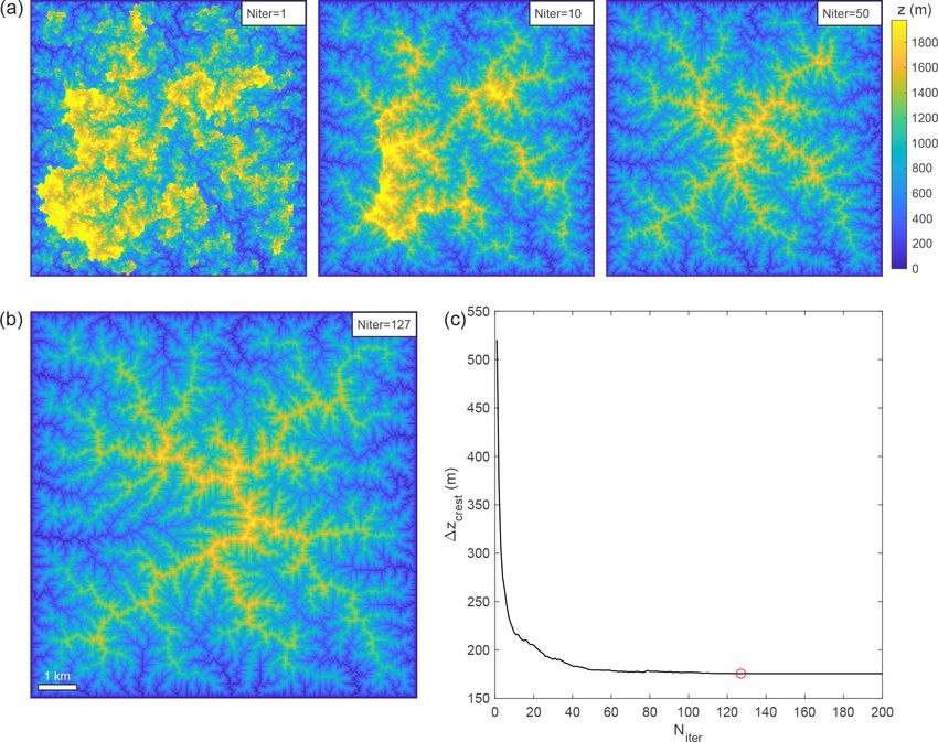
P. Steer: Short communication: Analytical models for 2D landscape evolution                                                         1241

                                                                     convergence of this iterative procedure, I define the degree of
                                                                     crest disequilibrium 1zcrest as being the average of the abso-
                                                                     lute difference of elevation between crest nodes of juxtapos-
                                                                     ing catchments. I find that 1zcrest follows a rapid decay with
                                                                     Niter until reaching a slower decay phase when Niter ≥ 40.
                                                                     1zcrest never reaches 0 m, even after 100 iterations, as dif-
                                                                     ferences of elevation can remain along the two sides of the
                                                                     crests, as in other LEMs, due to the non-continuity of the spa-
                                                                     tial discretization for grid-based models (Fig. 2c). However,
                                                                     the model reaches a stable solution at Niter = 127. Note that
                                                                     running the same model but with a different initial topogra-
                                                                     phy leads to a variability of this required number of iterations
                                                                     due to the initial configuration of the flow network.
Figure 1. Overview of the algorithms used for the (a) steady-state
                                                                        Changing U , K and L while keeping npt constant does
and (b) dynamic simulations.                                         not lead to a significant change in the number of iterations
                                                                     required to reach steady state (Fig. 3). This shows that the
                                                                     convergence of this algorithm is independent of the model
ceiver node τR (l) and its elevation zR (l):                         parametrization. However, increasing the number of points
                                                                     npt leads to an increase in the number of iterations required to
z(l) =zR (l) + U (l) (τ (l) − τR (l)) for l > 0,                     reach steady state, which scales with n0.5   pt , or in other words
      and z(0) = zbase .                                      (5)    with the number of nodes in one of the horizontal dimen-
                                                                     sions (Fig. 3). This scaling emerges due to the more numer-
Obviously, this operation needs to be performed iteratively          ous numbers of local (i.e. among direct neighbours) permu-
and in the correct node order, from the outlet node towards          tations of the crest location required to reach a stable fluvial
the upstream direction using the node stack or graph (Braun          organization when increasing npt .
and Willett, 2013; Schwanghart and Scherler, 2014). Ignor-              The new algorithm developed in Salève presents sig-
ing hillslope processes, I use this solution to attempt com-         nificant advantages compared to finite-difference schemes,
puting the steady-state topography with Salève in a single           which are fundamentally limited by the time step 1t that
iteration (Fig. 2). The initial topography consists of a flat sur-   must respect the Courant conditions 1t < k1x/max(C(l)),
face with a random noise discretized by a regular grid. I use        with k equal to ∼ 0.1 or to 100 for explicit or implicit
m = 0.5, corresponding to the classical unit stream power,           schemes, respectively (e.g. Braun and Willett, 2013). There-
U = 10 mm yr−1 , K 0 = 1 × 10⁻⁶ yr−1 , r = 5/365 m d−1 and           fore, these finite-difference solutions are doomed to use
a square model domain of extent L = 10 km with a reso-               shorter time steps and a larger number of iterations when
lution of 50 m, corresponding to npt = 40.401 points. Flow           considering finer resolutions. On the contrary, this analyt-
over the topography is computed using the single-flow algo-          ical LEM converges towards steady state with roughly the
rithm provided by TopoToolbox (Schwanghart and Scherler,             same number of iterations, independently of the celerity C(l),
2014), which efficiently exploits the directed acyclic graph         which is set by K, A (i.e. L2 ) and m. The number of required
structure of the flow network (Phillips et al., 2015).               iterations, however, increases with n0.5  pt , which is equivalent
   The obtained solution looks very roughly like a clas-             to an increase with decreasing 1x = L/n0.5      pt when L is con-
sical steady-state topography, and yet it is not strictly at         stant, as in classical finite-difference schemes. Moreover, this
steady state (Fig. 2). Indeed, during this first iteration, the      steady-state modelling approach is compatible with spatially
scheme used (Fig. 1a) imposes the constraint that rivers de-         variable U , K and r.
velop over the flow network defined by the initial topogra-
phy and, in turn, does not ensure that the nodes located on
                                                                     4   A 2D dynamical model with analytical accuracy
the same crest of two juxtaposing catchments share the same
response time or the same elevation. This leads to an exces-         I now explore the use of this analytical model in dynamic
sive elevation as some rivers have planar length greater than        simulations with Salève (Fig. 1b). I first consider the case
predicted. This is the main limit of this 1D algorithm that          of potentially heterogeneous but constant uplift rate U (l). A
cannot ensure the optimality of the 2D organization of the           transient solution for river elevation z(l, t) at a specific time t
river network at steady state after only one iteration (Fig. 2).     can be computed using Eqs. (4) or (5) by simply thresholding
   However, repeating this operation by computing the to-            the response time so that for every node τ (l, t) = min(τ (l), t).
pography and then updating the flow network (i.e. by com-            It results in the following:
puting the steepest slope, node order, and drainage area or
discharge) after each iteration leads to a steady-state topog-       z(l, t) =zR (l, t) + U (l) (τ (l, t) − τR (l, t)) for l > 0,
raphy after a few tens of iterations Niter (Fig. 2). To assess the            and z(0, t) = zbase .                                  (6)

https://doi.org/10.5194/esurf-9-1239-2021                                                 Earth Surf. Dynam., 9, 1239–1250, 2021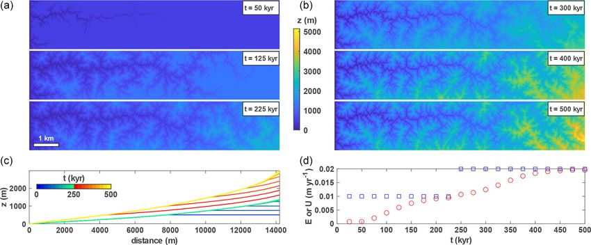
1242                                              P. Steer: Short communication: Analytical models for 2D landscape evolution

Figure 2. Modelled steady-state topographies obtained after (a) 1 (left panel), 10 (middle panel) and 50 (right panel) iterations. (b) The
steady-state topography is obtained after 127 iterations. (c) Convergence of the iterative algorithm inferred from the degree of crest dis-
equilibrium 1zcrest , computed as the average of the absolute difference of elevation between crest nodes of juxtaposing catchments. Red
dot indicates model shown in panel (b). Note that in panel (a), the colour map is bounded by the maximum elevation of the steady-state
topography shown in panel (b).

This solution therefore enables computation of the time evo-            elevation is set by the flow network. In other words, Salève
lution of a landscape under potentially heterogeneous erodi-            does not fully guarantee the time continuity of the topogra-
bility, uplift and runoff (or precipitation) rates. Thresholding        phy through successive time steps, despite practically having
the response time enforces that the uplift rate is considered           a limited impact on model behaviour as I will demonstrate
null before the beginning of the simulation. The limitation             later.
of non-optimality of the planar organization of flow network               I here run a simulation, using the same parameters as
remains as in the steady-state solution. However, this limita-          in the steady-state simulation, over a duration of 500 kyr
tion can be solved by simply updating the river network, the            (Fig. 4). The time steps 1t = 2 and 0.2 kyr correspond to
node order, the steepest slope and water discharge after each           about 45 and 4.5 times the Courant condition, respectively.
time step, as in any other LEMs. As the time step is not con-           Because implicit finite-difference solutions to the SPIM also
strained by numerical stability issues, such as the Courant             remain numerically stable for time steps longer than the one
condition, it can be chosen only based on the rate of flow              imposed by the Courant condition, I also run simulations us-
network reorganization linked to river capture and piracy.              ing an implicit solution with the same parameters and time
Note, however, that in the dynamic Salève models, flow net-             steps and compare them to the results of the Salève simula-
work reorganization will lead to an immediate topographic               tions. The implicit solution is computed following Eq. (22) in
reorganization, to respect Eq. (6). Indeed, time evolution of           Braun and Willett (2013). I also compare Salève with results
the elevation in Salève should not be seen as a continuous              obtained with an implicit solution using a time step 1t =
time evolution of a same topography, which would evolve by              0.002 kyr, corresponding to a Courant condition of 0.45.
erosion under different time and space distributions of water              The final topographies, i.e. at steady state, obtained with
discharge (e.g. as in other LEMs), but as a succession of to-           Salève or with the implicit solution share roughly the same
pographic realizations which respect that the distribution of           statistical properties in terms of vertical and horizontal orga-

Earth Surf. Dynam., 9, 1239–1250, 2021                                                    https://doi.org/10.5194/esurf-9-1239-2021
P. Steer: Short communication: Analytical models for 2D landscape evolution                                                     1243

                                                                      models continues to evolve after steady state, in particular the
                                                                      maximum elevation max(z), with larger variations for mod-
                                                                      els with longer time steps, which occurs due to catchment
                                                                      reorganization and numerical noise.
                                                                         Moreover, erosion rates E first increase more slowly and
                                                                      then more rapidly in Salève than with the implicit solu-
                                                                      tions before reaching steady state (Fig. 3d). In particular,
                                                                      the second phase is due to longer upstream distances and
                                                                      erosional response times in the topographies simulated with
                                                                      the implicit solution than with Salève (Fig. 3f). This is at
                                                                      least partly due to the dependency of the transient phase du-
                                                                      ration on 1t for finite-difference models (Braun and Wil-
                                                                      lett, 2013). Geometrically, longer transient phases are as-
                                                                      sociated with fluvial networks with longer upstream dis-
                                                                      tances, i.e. distances to the outlet, in the implicit models
                                                                      with longer time steps compared to implicit models with
                                                                      shorter time steps or to Salève models (Fig. 3e). These re-
                                                                      sults also show that the response time of the landscapes is
                                                                      shorter than with other 2D LEMs as it is equal to the 1D re-
                                                                      sponse time, based on the flow network length at steady state,
                                                                      when the time step used is sufficiently short to allow progres-
                                                                      sive reorganization of the fluvial network (e.g. model with
                                                                      1t = 0.2 kyr).
                                                                         Erosion rates in Salève, calculated by differencing eleva-
                                                                      tion between successive time steps and subtracting the con-
                                                                      tribution of uplift, are significantly more variable, in partic-
                                                                      ular for the model with the shorter time step 1t = 0.2 kyr
                                                                      than with the implicit solutions. This variability highlights
                                                                      phases of fluvial network reorganization which lead to im-
                                                                      mediate topographic reorganization, due to time discontinu-
                                                                      ity, and therefore to an immediate increase in erosion rates.
Figure 3. Influence of model parameters and geometry on the con-         In terms of horizontal organization, all the Salève and im-
vergence towards a steady-state landscape. (a) Uplift rate U was
                                                                      plicit models lead to the same Hack’s law (Hack, 1957),
varied between 10−4 and 1 m yr−1 . (b) Erodibility K was varied
                                                                      which relates, through a power-law relationship, the down-
between 1 × 10⁻⁷ and 1 × 10⁻³ yr−1 . (c) Model length L was var-
ied between 0.1 and 100 km. (d) The number of model points npt        stream maximum river length Lr with catchment area: Lr ∝
was varied between 1.2 × 10³ and 0.4 × 10⁶ . (e) The relationship
                                                                      Ah . A least-square fitting gives an exponent h of 0.65 ±
between the number of iterations required to reach steady state and   0.01 for Salève and the implicit models at steady state,
npt follows a power law with an exponent 0.5 (blue line).             with no dependency over 1t. In terms of vertical organiza-
                                                                      tion, the slope–discharge relationship obtained with Salève
                                                                      at steady state fits perfectly with the predicted one, S =
                                                                      (U/K)1/n Q−m/n , while the implicit solution shows a signif-
nization. The time evolution of the mean elevation (mean(z))          icant spread, in particular at low drainage area or discharge,
and maximum elevation (max(z)) is similar in all the mod-             which increases with 1t (Fig. 3d). Using 1t = 0.02 instead
els, even if the steady-state value is higher by ∼ 50 for             of 2 kyr leads to a slightly better consistency between the im-
mean(z) and ∼ 500 m for max(z), with the implicit solution            plicit and Salève solution, including the slope–discharge re-
(Fig. 4c). Moreover, the fluvial network and hence the to-            lationship and the temporal evolution of elevation.
pography modelled with Salève reach a stable configuration
once at steady state, with no subsequent vertical or horizon-
tal changes. Topographic stability occurs when the model              5   Application: time-variable uplift and knickpoint
time t becomes greater or equal to the response time τ (l)                propagation
of all the model nodes, and in particular the ones located on
crests (Fig. 4b). This is particularly true if 1t is small enough     I now investigate the case of time-variable but homogeneous
to allow the horizontal organization of the fluvial network           uplift rate U (t). Following Royden and Taylor Perron (2013),
to evolve concomitantly with its vertical component. On the           this case leads to additional complexity as the uplift rate,
contrary, the topography simulated by the finite-difference           when the slope patches were initiated, must be tracked during

https://doi.org/10.5194/esurf-9-1239-2021                                               Earth Surf. Dynam., 9, 1239–1250, 2021
1244 P. Steer: Short communication: Analytical models for 2D landscape evolution Figure 4. Dynamic behaviour of the Salève model. (a) Time evolution of the modelled topography after 50 (left panel), 150 (middle panel) and 500 kyr (right panel). Time evolution of the (b) max elevation, (c) mean elevation and (d) mean erosion rate for Salève, using a time step of 1t = 2 kyr (black line) and 0.2 kyr (dashed black line) and for the implicit solution with 1t = 2 kyr (blue line), 0.2 kyr (green line) and 0.02 kyr (red line). The uplift rate U is shown in panel (d) with a cyan line. (e) Slope–discharge distributions at steady state (at 500 kyr) for the three models compared to the predicted relationship (cyan line). No binning is done, and all the model nodes are represented in panel (d). (f) Histograms of upstream distances d (left panel) and response times τ (right panel) for the different models at steady state. upstream migration. In a LEM, this is performed by com- computed in the upstream direction, starting with the river puting, at the specific time t, what I refer to as the uplift outlets, as memory map Umem (l, t) = U (t − τ (l, t)). It is not equivalent z(l, t) =zR (l, t) + Umem (l, t) (τ (l, t) − τR (l, t)) for l > 0, to a classical uplift map and corresponds to the uplift rate when the slope patches were formed. I remind the reader and z(0, t) = zbase . (7) here that the response time is bounded by actual model time As in the heterogeneous uplift case, this solution is easily τ (l, t) = min(τ (l), t). The elevation at a time t is then simply implemented in a LEM by updating the river network and its Earth Surf. Dynam., 9, 1239–1250, 2021 https://doi.org/10.5194/esurf-9-1239-2021
P. Steer: Short communication: Analytical models for 2D landscape evolution                                                             1245

Figure 5. Dynamic evolution of the topography and knickpoint migration over 500 kyr. The initial uplift rate U = 10 mm yr−1 is doubled
after 250 kyr. (a) Topography before the increase in uplift at 50 (top panel), 125 (middle panel) and 225 kyr (bottom panel). (b) Topography
after the increase in uplift at 300 (top panel), 400 (middle panel) and 500 kyr (bottom panel). (c) Temporal evolution of the longest river
profile shown at every time step (except the first one), with the “winter” and “autumn” colour map showing river profiles before and after the
increase in uplift. (d) Temporal evolution of the uplift (blue squares) and erosion (red circles) rates.

properties after each time step. I also emphasize here that the          the knickpoint is also kept throughout its migration. I also
previous model example (Fig. 4) is already a specific case               highlight here that, due to the model setting with only one
of a time-variable uplift rate, with a change in uplift rate             outlet boundary, which limits river reorganization (and time
which occurs at the beginning of the simulation, leading in              discontinuity), erosion rates are smoother than in Fig. 4.
turn to a simpler formalism (Eq. 6). In the following, I focus
on demonstrating the ability of the model to simulate and
track knickpoints.                                                       6   Solving for river and hillslope dynamics
   Discrete temporal changes in uplift rates or in base-level
elevation can lead to sharp ruptures in the slope of river pro-          In previous sections, I have considered the steady-state and
files, generally referred to as knickpoints (e.g. Rosenbloom             dynamic solutions of landscapes subjected only to river ero-
and Anderson, 1994; Whipple and Tucker, 1999; Steer et al.,              sion following the SPIM. However, these analytical solutions
2019). Finite-difference solutions to the stream power equa-             can be extended to simulate the dynamics and morphology of
tion inherently lead to a progressive numerical diffusion of             colluvial valleys and hillslopes. Indeed, a power-law scaling
knickpoints during their migration, even with n = 1, while               for the slope–area relationship is observed in colluvial val-
the algorithm developed here preserves the shape of knick-               leys, which suggest they could obey a similar erosion law
points. To illustrate this advantage, I run a simulation with the        as Eq. (1), but with different m and n exponents (Lague
same parameters as in the steady-state case, except that U is            and Davy, 2003). A solution with m = 0.24 and n = 1, but
raised from 10 to 20 mm yr−1 at 250 kyr for a total model                considering a non-negligible incision threshold, was found
duration of 500 kyr (Fig. 5). Compared to previous models,               to best explain the geometry of colluvial valleys in the Si-
the model is here restricted to an extent of 10 km over 2 km,            walik Hills of Nepal for drainage area between 7 × 10⁻³
with only one boundary (left) that is considered as possible             and 1 km2 , representing the thresholds in drainage area be-
outlets for water. This setting limits fluvial network reorgani-         tween colluvial valleys and hillslopes or rivers, respectively
zation (or time discontinuity) and in turn allows for tracking           (Lague and Davy, 2003). Below the area transition between
geomorphological features during the evolution of the land-              colluvial valleys and hillslopes, the power-law scaling for the
scape. I use a time step of 25 kyr, which is about 500 times             slope–area relationship becomes flat, due to landsliding and
greater than the time step imposed by the Courant condition,             mass wasting processes, or reverts where hilltops are convex
clearly above the range of time steps compatible with nu-                (Ijjasz-Vasquez and Bras, 1995; Tarolli and Dalla Fontana,
merical solutions. Despite this, the knickpoints formed at the           2009). Once again, this hillslope domain could be geometri-
outlets of the model at 250 kyr, at the onset of the increase            cally modelled using the SPIM with different m and n, e.g.
in uplift rate, are accurately modelled, i.e. with analytical ac-        with m = 0 and n = 1, to model hillslopes following a critical
curacy, throughout their propagation (Fig. 5c). The shape of             angle of repose Sc . I do not argue here that these laws nec-
                                                                         essarily encapsulate the processes controlling colluvial and

https://doi.org/10.5194/esurf-9-1239-2021                                                    Earth Surf. Dynam., 9, 1239–1250, 2021
1246 P. Steer: Short communication: Analytical models for 2D landscape evolution
hillslope erosion (e.g. Tucker and Bras, 1998; Densmore et 7 Discussion and conclusion
al., 1998; Roering et al., 1999; Lague and Davy, 2013; Jean-
det et al., 2019) but that this framework can approximate the Based on previous analytical developments (e.g. Royden and
observed geometrical relationships between slope and area. Taylor Perron, 2013), I have designed a new method to solve
Practically, considering three different erosion laws, for for the steady-state topography or the dynamic evolution of a
river, colluvial valleys and hillslopes, simply requires chang- landscape in 2D, following the SPIM, with analytical preci-
ing the value of K, m and n in the definition of celerity in the sion. The model can solve in a single time step, using an iter-
response time equation (Eq. 3) for each of the different do- ative scheme, the steady-state topography of a landscape un-
mains, separated by thresholds in discharge or drainage area. der homogeneous or heterogenous conditions (i.e. uplift rate,
Keeping n = 1 for simplicity leads to the following set of re- erodibility and runoff). Iterations are required to optimize the
sponse time equations: planar organization of the river network and crest positions,
starting from a random network. The number of iterations
Zl required for the convergence of the scheme only depends on
1
τ (l) = dl 0 the number of nodes discretizing the surface topography and
K1 (l)A(l)m1
0 only scales with n0.5
pt , independently of other model parame-
ters. Moreover, the model can also solve for the dynamic evo-
for l < l1 ,
lution of a landscape under either heterogeneous but constant
Zl1 Zl or time-variable but homogeneous conditions. The dynamic
1 1
τ (l) = dl 0 + dl 0 and steady-state Salève models can solve for river, colluvial
K1 (l)A(l)m1 K2 (l)A(l)m2
0 l1 and hillslope erosion, if the associated erosion laws lead to
slope–area (or discharge) relationships that can be modelled
for l1 < l ≤ l2 ,
using a linear SPIM. The two main benefits of this new model
Zl1 Zl2 are (1) its analytical accuracy that enables suppression of nu-
1 1
τ (l) = dl 0 + dl 0 merical diffusion and, for instance, the maintenance of the
K1 (l)A(l)m1 K2 (l)A(l)m2
0 l1 shape of knickpoints and (2) the absence of an upper bound
for the time step that is not limited by the Courant condi-
Zl
1 tion. Contrary to any other state-of-the-art LEMs using the
+ dl 0
K3 (l)A(l)m3 SPIM (e.g. Braun and Willett, 2013; Carretier et al., 2016;
l2 Campforts et al., 2017; Hobley et al., 2017; Salles, 2018), the
for l > l2 , (8) time-stepping strategy in Salève can be chosen only based
on physical considerations, such as the rate of river network
where A(l1 ) and A(l2 ) are model parameters that define the reorganization, and not on numerical ones. All these advan-
threshold areas for river to colluvial valley and for colluvial tages make Salève unique in its ability to efficiently model
valley to hillslope transitions, and (K1 , m1 ), (K2 , m2 ), and landscape evolution. In addition to its use in landscape evolu-
(K3 , m3 ) are the K values and m exponents for rivers, col- tion modelling, Salève could offer new opportunities to gen-
luvial valleys and hillslopes, respectively. I emphasize here erate terrains for applications in computer graphics (e.g. Cor-
that the colluvial law used here is only inspired from the col- donnier et al., 2016); to infer the time and space evolution
luvial law described in Lague and Davy (2003), as it neglects of uplift by inverting landscapes in 2D (e.g. Pritchard et al.,
the incision threshold which lead to a non-linear behaviour. 2009; Roberts and White, 2010; Goren et al., 2014a; Fox et
Figure 6 shows the steady-state topographies obtained when al., 2014; Croissant and Braun, 2014) including river, collu-
considering river, colluvial and hillslope erosion. Consider- vial valleys, and hillslopes; to predict thermochronological
ing these additional erosion laws leads, as expected, to dif- ages from landscape evolution (e.g. Braun et al., 2014); or
ferent scaling in the slope–discharge relationships, separated to validate the accuracy of numerical schemes used in other
by thresholds in discharge or drainage area. These thresholds LEMs. The model is fast as it makes use of the optimized
should be chosen to ensure (1) the continuity of the slope– flow routing algorithm provided by TopoToolbox (Schwang-
discharge relationship and (2) the slope is equal to Sc when hart and Scherler, 2014).
A ≤ A(l2 ). I emphasize, once again, that the models devel- The developed scheme, that uses 1D analytical solutions,
oped here lead to slope–discharge relationships with exact is limited to flow networks that can be topologically classi-
accuracy, at steady state, due to the use of analytical solu- fied as 1D node stacks or graphs (Braun and Willett, 2013), as
tions. Other analytical solutions can be considered to account resulting from a steepest slope flow routing algorithm. This
for hillslope processes such as the one developed in the DAC excludes, for instance, recent models accounting for flow
model (Goren et al., 2014b). algorithms based on physical considerations (Davy et al.,
2017). The main limitation of this new approach is that re-
organizations of the river network, such as catchment piracy,
will not lead to transient phases of erosion, as the river el-
Earth Surf. Dynam., 9, 1239–1250, 2021 https://doi.org/10.5194/esurf-9-1239-2021P. Steer: Short communication: Analytical models for 2D landscape evolution 1247
Figure 6. Steady-state topographies obtained with Salève considering only (a) stream power incision (m = 0.5) in rivers (like in Fig. 1),
(b) stream power incision (m = 0.5) in rivers and colluvial erosion (m = 0.24), and (c) stream power incision in rivers (m = 0.5), colluvial
erosion (m = 0.24), and hillslopes following a critical slope (m = 0) of Sc = 30◦ . To better highlight relief, elevation is represented by
transparency over the raster of hillshade. (d) Slope–discharge distributions for these three models.
evation is directly updated to its optimal elevation for each tive to the location of the base-level condition. Moreover,
node where t ≤ τ (l, t). The response time of the modelled Salève is a purely detachment-limited model which does not
landscapes is therefore shorter than with other 2D LEMs as consider the role of sediment transport and deposition in
it is equal to the 1D response time based on the flow network landscape dynamics. Only the linear SPIM with n = 1 has
length at steady state. Moreover, the flow network topology been considered in this study, while some observations sup-
is updated at every iteration or time step, in the steady-state port non-linear models with greater values for n (e.g. Lague,
or dynamic modes, respectively, while other strategies, based 2014). These limitations also emphasize that analytical so-
on physical criterion, could be adopted (Goren et al., 2014b). lutions to landscape dynamics, such as Salève, represent a
If many dynamic LEMs use the same approach (e.g. Braun complementary approach to other “numerical” LEMs, which
and Willett, 2013), this is a critical aspect of the convergence are in essence more versatile and allow for tackling coupled
speed and computational time in the steady-state mode, and or complex scientific problems which characterize geomor-
future work should focus on accelerating it. phological systems.
The Salève model is also not designed for horizontal tec- Extending the Salève algorithm to non-linear SPIMs rep-
tonic displacement (e.g. Braun and Sambridge, 1997; Steer resents a challenging and non-trivial perspective that requires
et al., 2011; Miller et al., 2007) that displaces nodes rela- accounting for more complex analytical solutions with over-
https://doi.org/10.5194/esurf-9-1239-2021 Earth Surf. Dynam., 9, 1239–1250, 20211248 P. Steer: Short communication: Analytical models for 2D landscape evolution
lapping or stretching river profiles for n > 1 or n < 1, re- Review statement. This paper was edited by Greg Hancock and
spectively (Royden and Taylor Perron, 2013). Using Salève reviewed by Sebastien Carretier and Liran Goren.
to simulate the impact of both a heterogeneous and time-
variable uplift rate has not been attempted and might also
result in convergence issues. Moreover, using an even more
References
efficient algorithm to route water also represents a promising
avenue (e.g. Barnes et al., 2014). This is critical for Salève Barnes, R., Lehman, C., and Mulla, D.: Priority-flood: An optimal
that can use a time step much greater than the Courant con- depression-filling and watershed-labeling algorithm for digital
dition and for which the main computational limit is the flow elevation models, Comput. Geosci., 62, 117–127, 2014.
routing algorithm. Therefore, no computational time bench- Braun, J. and Sambridge, M.: Modelling landscape evolution on ge-
mark was done for this new model, as the computation of ological time scales: a new method based on irregular spatial dis-
elevation changes, even on large grids, is negligible com- cretization, Basin Res., 9, 27–52, 1997.
pared to flow routing. In turn, solving for individual time Braun, J. and Willett, S. D.: A very efficient O(n), implicit and
steps in this model takes a similar amount of computational parallel method to solve the stream power equation governing
time as in other similar LEMs using the same flow routing fluvial incision and landscape evolution, Geomorphology, 180,
170–179, 2013.
algorithm (e.g. Braun and Willett, 2013; Schwanghart and
Braun, J., Simon-Labric, T., Murray, K. E., and Reiners, P. W.: To-
Scherler, 2014). Yet, the advantage of this new model is its pographic relief driven by variations in surface rock density, Nat.
ability to use longer time steps while preserving analytical Geosci., 7, 534–540, 2014.
accuracy and consistency. Lastly, Salève represents the first Campforts, B. and Govers, G.: Keeping the edge: A numerical
attempt to use analytical solutions to model the dynamics of method that avoids knickpoint smearing when solving the stream
landscapes in 2D using the SPIM. Because little modifica- power law, J. Geophys. Res.-Earth, 120, 1189–1205, 2015.
tions are required to implement this solution in other LEMs, I Campforts, B., Schwanghart, W., and Govers, G.: Accurate simu-
believe the strategy developed in this paper could be adapted lation of transient landscape evolution by eliminating numerical
and further developed to make LEMs more efficient and ac- diffusion: the TTLEM 1.0 model, Earth Surf. Dynam., 5, 47–66,
curate. https://doi.org/10.5194/esurf-5-47-2017, 2017.
Carretier, S. and Lucazeau, F.: How does alluvial sedimentation at
range fronts modify the erosional dynamics of mountain catch-
ments?, Basin Res., 17, 361–381, 2005.
Code availability. A MATLAB version of the
Carretier, S., Martinod, P., Reich, M., and Goddéris, Y.: Modelling
model can be accessed through a Zenodo repository:
sediment clasts transport during landscape evolution, Earth Surf.
https://doi.org/10.5281/zenodo.4686733 (Steer, 2021). It is
Dynam., 4, 237–251, 2016.
delivered with a routine to solve for the stream power law using an
Cordonnier, G., Braun, J., Cani, M. P., Benes, B., Galin, E., Pey-
implicit finite-difference solution.
tavie, A., and Guérin, E.: Large scale terrain generation from
tectonic uplift and fluvial erosion, Comput. Graph. Forum, 35,
165–175, 2016.
Competing interests. The author declares that there is no con- Croissant, T. and Braun, J.: Constraining the stream power law:
flict of interest. a novel approach combining a landscape evolution model
and an inversion method, Earth Surf. Dynam., 2, 155–166,
https://doi.org/10.5194/esurf-2-155-2014, 2014.
Disclaimer. Publisher’s note: Copernicus Publications remains Croissant, T., Lague, D., Steer, P., and Davy, P.: Rapid post-
neutral with regard to jurisdictional claims in published maps and seismic landslide evacuation boosted by dynamic river width,
institutional affiliations. Nat. Geosci., 10, 680–684, 2017.
Croissant, T., Steer, P., Lague, D., Davy, P., Jeandet, L., and Hilton,
R. G.: Seismic cycles, earthquakes, landslides and sediment
Acknowledgements. The two reviewers, Liran Goren and fluxes: Linking tectonics to surface processes using a reduced-
Sébastien Carretier, as well as the editor, Joshua West, and asso- complexity model, Geomorphology, 339, 87–103, 2019.
ciate editor, Greg Hancock, are acknowledged for their constructive Davy, P., Croissant, T., and Lague, D.: A precipiton method to cal-
comments that helped with improving this article. I am also grate- culate river hydrodynamics, with applications to flood prediction,
ful to Sean Willett for his insightful comments on an earlier version landscape evolution models, and braiding instabilities, J. Geo-
of this article. I thank Dimitri Lague, Philippe Davy, Jean Braun, phys. Res.-Earth, 122, 1491–1512, 2017.
Boris Gailleton, Joris Heyman, Alain Crave, Thomas Croissant and Densmore, A. L., Ellis, M. A., and Anderson, R. S.: Landsliding and
Edwin Baynes for their helpful comments and for discussions about the evolution of normal-fault-bounded mountains, J. Geophys.
this work. Res.-Solid, 103, 15203–15219, 1998.
Fox, M., Goren, L., May, D. A., and Willett, S. D.: Inversion of
fluvial channels for paleorock uplift rates in Taiwan, J. Geophys.
Financial support. This research has been supported by the Res.-Earth, 119, 1853–1875, 2014.
H2020 European Research Council (grant no. 803721). Freeman, T. G.: Calculating catchment area with divergent flow
based on a regular grid, Comput. Geosci., 17, 413–422, 1991.
Earth Surf. Dynam., 9, 1239–1250, 2021 https://doi.org/10.5194/esurf-9-1239-2021P. Steer: Short communication: Analytical models for 2D landscape evolution 1249 Goren, L.: A theoretical model for fluvial channel response time Phillips, J. D., Schwanghart, W., and Heckmann, T.: Graph theory during time-dependent climatic and tectonic forcing and its in- in the geosciences, Earth-Sci. Rev., 143, 147–160, 2015. verse applications, Geophys. Res. Lett., 43, 10753–10763, 2016. Pritchard, D., Roberts, G. G., White, N. J., and Richardson, C. Goren, L., Fox, M., and Willett, S. D.: Tectonics from fluvial to- N.: Uplift histories from river profiles, Geophys. Res. Lett., 36, pography using formal linear inversion: Theory and applications L24301, https://doi.org/10.1029/2009GL040928, 2009. to the Inyo Mountains, California, J. Geophys. Res.-Earth, 119, Quinn, P. F. B. J., Beven, K., Chevallier, P., and Planchon, O.: The 1651–1681, 2014a. prediction of hillslope flow paths for distributed hydrological Goren, L., Willett, S. D., Herman, F., and Braun, J.: Coupled modelling using digital terrain models, Hydrol. Process., 5, 59– numerical–analytical approach to landscape evolution modeling, 79, 1991. Earth Surf. Proc. Land., 39, 522–545, 2014b. Roberts, G. G. and White, N.: Estimating uplift rate histories from Hack, J. T.: Studies of longitudinal profiles in Virginia and Mary- river profiles using African examples, J. Geophys. Res.-Solid, land, U.S. Geol. Surv. Prof. Pap., 294, 45–97, 1957. 115, B02406, https://doi.org/10.1029/2009JB006692, 2010. Hobley, D. E. J., Adams, J. M., Nudurupati, S. S., Hutton, E. W. Roering, J. J., Kirchner, J. W., and Dietrich, W. E.: Evidence for H., Gasparini, N. M., Istanbulluoglu, E., and Tucker, G. E.: Cre- nonlinear, diffusive sediment transport on hillslopes and impli- ative computing with Landlab: an open-source toolkit for build- cations for landscape morphology, Water Resour. Res., 35, 853– ing, coupling, and exploring two-dimensional numerical mod- 870, 1999. els of Earth-surface dynamics, Earth Surf. Dynam., 5, 21–46, Rosenbloom, N. A. and Anderson, R. S.: Hillslope and channel evo- https://doi.org/10.5194/esurf-5-21-2017, 2017. lution in a marine terraced landscape, Santa Cruz, California, J. Howard, A. D.: A detachment-limited model of drainage basin evo- Geophys. Res.-Solid, 99, 14013–14029, 1994. lution, Water Resour. Res., 30, 2261–2285, 1994. Royden, L. and Taylor Perron, J.: Solutions of the stream power Howard, A. D. and Kerby, G.: Channel changes in badlands, Geol. equation and application to the evolution of river longitudinal Soc. Am. Bull., 94, 739–752, 1983. profiles, J. Geophys. Res.-Earth, 118, 497–518, 2013. Howard, A. D., Dietrich, W. E., and Seidl, M. A.: Modeling fluvial Salles, T.: eSCAPE: parallel global-scale landscape erosion on regional to continental scales, J. Geophys. Res.-Solid, evolution model, J. Open Source Softw., 3, 964, 99, 13971–13986, 1994. https://doi.org/10.21105/joss.00964, 2018. Ijjasz-Vasquez, E. J. and Bras, R. L.: Scaling regimes of local slope Schwanghart, W. and Scherler, D.: Short Communication: Topo- versus contributing area in digital elevation models, Geomor- Toolbox 2 – MATLAB-based software for topographic analysis phology, 12, 299–311, 1995. and modeling in Earth surface sciences, Earth Surf. Dynam., 2, Jeandet, L., Steer, P., Lague, D., and Davy, P.: Coulomb mechan- 1–7, https://doi.org/10.5194/esurf-2-1-2014, 2014. ics and relief constraints explain landslide size distribution, Geo- Steer, P.: philippesteer/Saleve_regular: (Version v1), Zenodo phys. Res. Lett., 46, 4258–4266, 2019. [code], https://doi.org/10.5281/zenodo.4686733, 2021. Lague, D.: The stream power river incision model: evidence, theory Steer, P., Cattin, R., Lavé, J., and Godard, V.: Surface Lagrangian and beyond, Earth Surf. Proc. Land., 39, 38–61, 2014. Remeshing: A new tool for studying long term evolution of Lague, D. and Davy, P.: Constraints on the long-term colluvial ero- continental lithosphere from 2D numerical modelling, Comput. sion law by analyzing slope-area relationships at various tectonic Geosci., 37, 1067–1074, 2011. uplift rates in the Siwaliks Hills (Nepal), J. Geophys. Res.-Solid, Steer, P., Simoes, M., Cattin, R., and Shyu, J. B. H.: Erosion in- 108, 2129, https://doi.org/10.1029/2002JB001893, 2003. fluences the seismicity of active thrust faults, Nat. Commun., 5, Lavé, J.: Analytic solution of the mean elevation of a watershed 5564, https://doi.org/10.1038/ncomms6564, 2014. dominated by fluvial incision and hillslope landslides, Geophys. Steer, P., Croissant, T., Baynes, E., and Lague, D.: Statisti- Res. Lett., 32, L11403, https://doi.org/10.1029/2005GL022482, cal modelling of co-seismic knickpoint formation and river 2005. response to fault slip, Earth Surf. Dynam., 7, 681–706, Luke, J. C.: Mathematical models for landform evolution, J. Geo- https://doi.org/10.5194/esurf-7-681-2019, 2019. phys. Res., 77, 2460–2464, 1972. Tarolli, P. and Dalla Fontana, G.: Hillslope-to-valley transition mor- Luke, J. C.: Special solutions for nonlinear erosion problems, J. phology: New opportunities from high resolution DTMs, Geo- Geophys. Res., 79, 4035–4040, 1974. morphology, 113, 47–56, 2009. Luke, J. C.: A note on the use of characteristics in slope evolution Thieulot, C., Steer, P., and Huismans, R. S.: Three-dimensional nu- models, Z. Geomorph. Supp., 25, 114–119, 1976. merical simulations of crustal systems undergoing orogeny and Miller, S. R., Slingerland, R. L., and Kirby, E.: Char- subjected to surface processes, Geochem. Geophy. Geosy., 15, acteristics of steady state fluvial topography above 4936–4957, 2014. fault-bend folds, J. Geophys. Res.-Earth, 112, F04004, Tucker, G. E. and Bras, R. L.: Hillslope processes, drainage density, https://doi.org/10.1029/2007JF000772, 2007. and landscape morphology, Water Resour. Res., 34, 2751–2764, Molnar, P. and England, P.: Late Cenozoic uplift of mountain ranges 1998. and global climate change: chicken or egg?, Nature, 346, 29–34, Tucker, G. E. and Whipple, K. X.: Topographic outcomes 1990. predicted by stream erosion models: Sensitivity analysis O’Callaghan, J. F. and Mark, D. M.: The extraction of drainage net- and intermodel comparison, J. Geophys. Res., 107, 2179, works from digital elevation data, Comput. Vis. Graph. Image https://doi.org/10.1029/2001JB000162, 2002. Process., 28, 323–344, 1984. Weissel, J. K. and Seidl, M. A.: Inland propagation of erosional Pelletier, J.: Quantitative modeling of earth surface processes, Cam- escarpments and river profile evolution across the southeast Aus- bridge University Press, Cambridge, 2008. https://doi.org/10.5194/esurf-9-1239-2021 Earth Surf. Dynam., 9, 1239–1250, 2021
1250                                             P. Steer: Short communication: Analytical models for 2D landscape evolution

 tralian passive continental margin, Geophys. Monogr., 107, 189–    Whipple, K. X.: The influence of climate on the tectonic
 206, 1998.                                                           evolution of mountain belts, Nat. Geosci., 2, 97–104,
Whipple, K. X. and Tucker, G. E.: Dynamics of the stream-power        https://doi.org/10.1038/ngeo413, 2009.
 river incision model: Implications for height limits of mountain   Willett, S. D.: Orogeny and orography: The effects of erosion on the
 ranges, landscape response timescales, and research needs, J.        structure of mountain belts, J. Geophys. Res.-Solid, 104, 28957–
 Geophys. Res.-Solid, 104, 17661–17674, 1999.                         28981, 1999.

Earth Surf. Dynam., 9, 1239–1250, 2021                                                https://doi.org/10.5194/esurf-9-1239-2021
You can also read