A model study of the seasonal mixed layer heat budget in the equatorial Atlantic
←
→
Page content transcription
If your browser does not render page correctly, please read the page content below
JOURNAL OF GEOPHYSICAL RESEARCH, VOL. 111, C06014, doi:10.1029/2005JC003157, 2006

A model study of the seasonal mixed layer
heat budget in the equatorial Atlantic
Anne-Charlotte Peter,1 Matthieu Le Hénaff,2 Yves du Penhoat,1 Christophe E. Menkes,2
Frédéric Marin,1 Jérôme Vialard,2 Guy Caniaux,3 and Alban Lazar2
Received 11 July 2005; revised 12 November 2005; accepted 17 February 2006; published 13 June 2006.

[1] In the present study, the physical processes that control the seasonal cycle of sea
surface temperature in the tropical Atlantic Ocean are investigated. A high-resolution
ocean general circulation model is used to diagnose the various contributions to the mixed
layer heat budget. The simulation reproduces the main features of the circulation and
thermal structure of the tropical Atlantic. A close examination of the mixed layer heat
budget is then undertaken. At a first order, the mixed layer temperature balance in the
equatorial band results from cooling by vertical processes and heating by atmospheric heat
fluxes and eddies (mainly tropical instability waves). Cooling by subsurface processes is
the strongest in June–August, when easterlies are strong, with a second maximum in
December. Heating by the atmosphere is maximum in February–March and September–
October, whereas eddies are most active in boreal summer. Unlike previous observational
studies, horizontal advection by low-frequency currents plays here only a minor role in the
heat budget. Off equator, the sea surface temperature variability is mainly governed by
atmospheric forcing all year long, except in the northeastern part of the basin where strong
eddies generated at the location of the thermal front significantly contribute to the heat
budget in boreal summer. Finally, comparisons with previously published heat budgets
calculated from observations show good qualitative agreement, except that subsurface
processes dominate the cooling over zonal advection in the present study.
Citation: Peter, A.-C., M. Le Hénaff, Y. du Penhoat, C. E. Menkes, F. Marin, J. Vialard, G. Caniaux, and A. Lazar (2006), A model
study of the seasonal mixed layer heat budget in the equatorial Atlantic, J. Geophys. Res., 111, C06014, doi:10.1029/2005JC003157.

1. Introduction                                                            7C [Houghton and Colin, 1986] in the eastern part of the
                                                                           equatorial basin. The resulting temperature gradient be-
  [2] The tropical Atlantic Ocean is a place of strong air-sea
                                                                           tween the cold water along the equator and the warmer
interactions, and much of the upper ocean variability is
                                                                           water north of it might influence the onset of the African
associated with the meridional displacement of the Inter-
                                                                           monsoon through the intensification of the southerly winds
Tropical Convergence Zone (ITCZ), which modulates the
                                                                           in the Gulf of Guinea [Okumura and Xie, 2004]. SST is
trade winds [Xie and Carton, 2004]. Contrary to the Pacific
                                                                           thought to have a strong impact on the meridional gradient
Ocean where the El Niño Southern Oscillation signal
                                                                           of moist static energy in the atmospheric boundary layer
dominates the variability, the annual cycle prevails in the
                                                                           between the Gulf of Guinea (GG) and the continent, and the
Atlantic Ocean. One striking feature of the seasonal cycle is
                                                                           GG provides 20% of the water vapor to the African
the appearance at the surface of cold water in boreal spring
                                                                           Monsoon flux [Fontaine et al., 2003].
in the vicinity of the equator. This cold tongue appears from
                                                                             [3] Many studies of the annual cycle of the ocean vertical
the coast of Africa, extending to roughly 15W when the
                                                                           structure in the tropical Atlantic, with observations
ITCZ moves northward in boreal spring, and reaches its
                                                                           [Houghton, 1991] and with models [Busalacchi and Picaut,
maximum in June at 10W at the equator [Carton and Zhou,
                                                                           1983; Du Penhoat and Treguier, 1985; Philander and
1997]. Sea Surface Temperature (SST) thus exhibits a
                                                                           Pacanowski, 1986] have shown that the annual cycle of
marked seasonal signal, which amplitude can reach up to
                                                                           the thermocline (generally represented by the variability of
                                                                           the 20C isotherm depth, referred to hereafter as D20) is
    1
      Laboratoire d’Etudes en Géophysique et Océanographie Spatiales,    controlled by wind forcing on the basin scale. Following the
Centre National d’Etudes Spatiales, CNRS, Institut de Recherche Pour le    intensification of the trade winds, the currents increase and
Développement, Université Paul Sabatier, Toulouse, France.
    2
      Laboratoire d’Océanographie et du Climat: Expérimentation et       the thermocline shoals in the eastern part of the basin
Approches Numériques, CNRS, Université Pierre et Marie Curie, Institut   [Houghton, 1989], which results in the formation of a cold
de Recherche Pour le Développement, Museum National d’Histoire            tongue in the equatorial upwelling region with colder water
Naturelle, Paris, France.                                                  closer to the surface.
    3
      Centre National Recherche Météorologique, Toulouse, France.
                                                                             [4] The seasonal evolution and maintenance of the cold
Copyright 2006 by the American Geophysical Union.                          tongue also depend on dynamic processes, such as vertical
0148-0227/06/2005JC003157$09.00                                            and horizontal advection, vertical mixing, and heat flux

                                                                    C06014                                                       1 of 16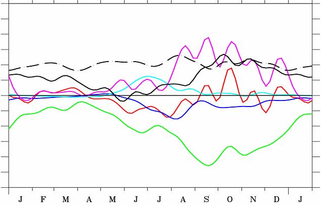
C06014                           PETER ET AL.: SEASONAL MIXED LAYER HEAT BUDGET                                           C06014

divergence associated with Tropical Instability Waves             first 200 m). It covers the Atlantic Ocean from the Drake
(TIWs), which are common to the Pacific and Atlantic              Passage to 30E and from Antarctica (75S) to 70N, with a
oceans.                                                           Mercator isotropic grid at 1/6 resolution at the equator.
  [5] In the equatorial Atlantic Ocean, a number of obser-        There are four open boundaries, at Drake Passage, at 30E
vational studies [e.g., Merle, 1980] and modeling studies         between Africa and Antarctica, in the Gulf of Cadiza and at
[Philander and Pacanowski, 1986] have addressed the               70N in the Nordic seas [Treguier et al., 2001].
causes of the annual cycle of SST. They found intense               [8] A horizontal biharmonic operator is used for lateral
warming by atmospheric heat fluxes, for both the mean             mixing of momentum with a coefficient of 5.5 1010 m4 s1
balance and the seasonal cycle. The vertical processes            at the equator, varying with the third power of the grid
(vertical advection, mixing, and entrainment) are the main        spacing. Mixing of temperature and salinity is done along
cooling terms balancing the warming by atmospheric fluxes,        isopycnals using a Laplacian operator, with a coefficient of
but horizontal advection is also a significant contributor.       150 m2 s1 at the equator, also varying in latitude with the
Foltz et al. [2003] (hereinafter referred to as FGCM) used a      grid spacing. The vertical mixing of momentum and tracers
variety of satellite and in situ data sources (data from Pilot    is calculated using a second-order closure model [Madec et
Research Moored Array in the Tropical Atlantic (PIRATA)           al., 1998]. In case of static instability, the vertical mixing
moorings) to examine the causes of the seasonal cycle of          coefficients are set to the large value of 1 m2 s1. An
SST in response to seasonally varying surface heating and         enhanced Laplacian mixing of momentum is added in the
winds, in the tropical Atlantic Ocean, through a heat budget      upper equatorial band so as to prevent the Equatorial Under
analysis. They characterized three different equatorial           Current (EUC) from being too intense [Michel and Treguier,
regions (corresponding to the location of three equatorial        2002]. The added Laplacian diffusion of momentum has a
moorings): (1) the western part of the basin near 35W in         constant coefficient 103 m2 s1 between 1N and 1S and
which the seasonal cycles of zonal heat advection, eddy           above 60 m, decaying to zero at 3 of latitude and 120 m
advection, entrainment and net surface heat flux all con-         depth. This additional mixing term accounts for inertial
tribute significantly to the seasonal SST variability, (2) the    instability processes that are not present in the model, at this
central equatorial region (23W), with a similar heat balance     spatial resolution [Richards and Edwards, 2003].
except that seasonal variations of latent heat and entrain-         [9] All surface forcing fields apart from the wind stress
ment cooling are significantly smaller, and (3) the eastern       are derived from the European Centre for Medium-Range
equatorial region (10W) where cooling from mean merid-           Weather Forecasts (ECMWF) Re-Analysis ERA-15 for the
ional advection and warming from eddy advection tend to           period covering 1990 to 1993 [Gibson et al., 1997], and
balance so that SST seasonal changes are mainly driven by         from the ECMWF analysis for the years 1994 to 2000. The
absorbed shortwave radiation.                                     non solar heat fluxes are formulated as suggested in Barnier
  [6] However, the observational studies cannot evaluate          et al. [1995], using a relaxation to the observed SST
explicitly every term of heat budget, in particular the           [Reynolds and Smith, 1994], with a feedback coefficient
vertical terms that are very difficult to compute directly.       taken equal to 40 W m2 K1, which corresponds to a
These studies are also subject to sampling error because of       relaxation timescale of 2 months for a 50 m mixed layer
the insufficient temporal and spatial resolution. This is         depth. A relaxation to a climatological sea surface salinity
especially true for the heat transported by TIWs that             with a similar timescale is added to the evaporation minus
requires high-resolution data sets to be resolved satisfacto-     precipitation fluxes which are formulated as a pseudo salt
rily [Jochum et al., 2005]. By using a model, a complete          flux, and include a river runoff [Treguier et al., 2001]. The
and consistent picture of the ocean circulation is given. This    wind stress forcing is derived from Earth Remote Sensing
allows a precise evaluation of all contributions to a closed      (ERS)1 – 2 wind scatterometers (http://www.ifremer.fr/
heat budget. In this study, the OPA-CLIPPER [Treguier et          cersat/) [Grima et al., 1999]. ERS winds were chosen instead
al., 2001] Ocean Global Circulation Model (OGCM) is used          of ECMWF because of the higher-quality wind forcing,
to assess the role of the different oceanic processes in the      especially in the eastern part of the basin (A. M. Treguier,
tropical Atlantic heat budget and to determine the mecha-         personal communication, 2004).
nisms responsible for the SST mean balance and seasonal             [10] A 3 year spin-up procedure is used as follows: The
cycle. The model characteristics, the mixed layer heat            model is run from 1990 to 1992 using heat and salt fluxes
budget equation, and the data sets used for the validation        from ECMWF, and the climatology of ERS wind stress
are introduced in section 2. In sections 3 and 4, the ocean       obtained by averaging years 1993 to 2000. Then, the model
state is described and validated, and the heat budget is          is forced by weekly ERS wind stress data between 1993 and
analyzed, respectively for the mean state and the seasonal        2000, and by daily ECMWF fluxes. More attention was
cycle. Results are then discussed in section 5 and summa-         paid to the heat budget in the equatorial basin for the years
rized in section 6.                                               1997 to 2000 away from the coastal regions (the model is
                                                                  not able to reproduce these particular dynamics, which are
2. Model and Methodology                                          beyond the scope of the present study).
2.1. Modeling Approach                                            2.2. Mixed Layer Heat Budget
  [7] The ocean model used in this study is the primitive           [11] This approach has already been used, for example, to
equation OGCM OPA 8.1 [Madec et al., 1998] in the                 investigate the SST balance in the tropical Pacific Ocean on
CLIPPER configuration [Treguier et al., 2001; Arhan et            seasonal to interannual timescales [Vialard et al., 2001] and
al., 2006]. This configuration uses z coordinates on the          the contributions to intraseasonal SST variability in the
vertical (42 geopotential vertical levels with 12 levels in the   Indian Ocean [Duvel et al., 2004]. In the present study,

                                                             2 of 16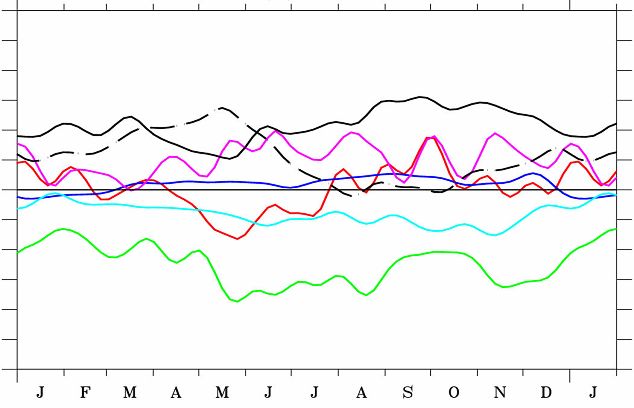
C06014 PETER ET AL.: SEASONAL MIXED LAYER HEAT BUDGET C06014
the mixed layer temperature equation is decomposed as include Brazil Current eddies, TIWs and intraseasonal equa-
described by Menkes et al. [2006]: torial wave activity. However, TIWs are the main contributors
to this eddy term, in agreement with a study in the Pacific
D E D E
[Menkes et al., 2006]. The dominant contributor to the
@t hTi ¼ u:@x T þ v:@y T u0 @x T0 v0 @y T0 þ hDl i
|fflfflfflfflfflffl{zfflfflfflfflfflffl} |fflfflfflfflfflffl{zfflfflfflfflfflffl} |fflfflfflfflfflfflfflfflfflfflfflfflfflfflfflfflfflfflfflfflfflfflfflffl{zfflfflfflfflfflfflfflfflfflfflfflfflfflfflfflfflfflfflfflfflfflfflfflffl} subsurface term proves to be the vertical diffusion at the base
a b c of the mixed layer, with a minor role for upwelling. This is due
ðKz @z TÞðz¼hÞ 1 to our computation of the heat budget over a time and space
@t h þ wðz¼hÞ hTi Tðz¼hÞ varying mixed layer. This contrasts with a heat budget
h h
|fflfflfflfflfflfflfflfflfflfflfflfflfflfflfflfflfflfflfflfflfflfflfflfflfflfflfflfflfflfflfflfflfflfflfflfflfflfflfflfflfflfflfflfflffl{zfflfflfflfflfflfflfflfflfflfflfflfflfflfflfflfflfflfflfflfflfflfflfflfflfflfflfflfflfflfflfflfflfflfflfflfflfflfflfflfflfflfflfflfflffl}
d calculated over a constant depth mixed layer in which vertical
Q* þ Qs 1 f ðz¼hÞ advection dominates vertical diffusion.
þ þ hðT hTiÞ@z wi ð1Þ
r0 Cp h |fflfflfflfflfflfflfflfflfflfflffl{zfflfflfflfflfflfflfflfflfflfflffl} 2.3. Validation
|fflfflfflfflfflfflfflfflfflfflfflfflfflfflfflfflffl{zfflfflfflfflfflfflfflfflfflfflfflfflfflfflfflfflffl} res
e [15] In order to validate the MLD, thermocline depth,
temperature vertical structure, Sea Level Anomalies (SLA)
with and currents in the model, different observation data sets were
used. TOPEX/Poseidon-ERS (T/P-ERS) SLA are used, on a
Z0 1/4 1/4 grid every 10 days. The SLA were built after
1
h i¼ dz removing the mean sea surface over 7 years (1993 –1999) [Le
h Traon et al., 1998]. The accuracy of this product is about 2 –
h
3 cm RMS in the Tropics. The PIRATA moored buoy array
[Servain et al., 1998] consist of ten moorings which measure
[12] Here, T is the temperature; u, v and w are respectively
subsurface temperatures at 11 depths between 1 and 500 m
the zonal, meridional and vertical currents, Kz the vertical
with 20 m spacing in the upper 140 m. The Tropical Atlantic
mixing coefficient for tracers, h the Mixed Layer Depth
Ocean Subsurface Temperature Atlas (TAOSTA) is an
(MLD), and Dl the lateral diffusion. The last term (e) on the
interannual database of vertical temperatures (0 – 500 m)
right hand side corresponds to the atmospheric forcing, Q*
between 1979 and 1999, over a domain extending from
and Qs are the nonsolar and solar components of the total
70W to 12E and 30S to 30N, with a 2 2 latitude-
heat flux, and f (z = h) is the fraction of the solar
longitude grid [Vauclair and Du Penhoat, 2001]. Modeled
shortwave that reaches the mixed layer depth h. A formu-
MLD are validated using the global mixed layer depth
lation including extinction coefficients (0.35 m and 23 m)
climatology from de Boyer Montégut et al. [2004] (herein-
is assumed for the downward irradiance [Paulson and
after referred to as dBM) available on a 2 2 spatial grid
Simpson, 1977]. Note that the flux term contains a damping
at a monthly resolution, and computed from the same density
term, proportional to the difference between the modeled
criterion as in CLIPPER. SST weekly mean maps from the
and the observed SST from Reynolds and Smith [1994]. The
TRMM Microwave Imager (TMI; see www.remss.com)
MLD is defined as the depth at which the density is equal to
radiometer between 1998 and 2000, at a resolution of
surface density plus 0.05 kg m3. The h.i represent a
0.25 are also used. Finally, Richardson and McKee
quantity integrated over the mixed layer.
[1984] (hereinafter referred to as RMK) provide a monthly
[13] To separate low- and high-frequency horizontal
climatology of ship drift – derived surface currents on a 1
advections, the 35-day Hanning-filtered low-frequency
1 grid within the region 20S – 20N, 10E–70W.
component of currents and temperature (denoted by over-
[16] The SLA spatial variability from the model is compa-
bars) are first computed offline, and are then integrated over
rable to T/P-ERS (Figure 1). Both low- and high-variability
the Mixed Layer (ML) (terms a and b in equation (1)).
regions are well located with comparable amplitude. How-
Higher-frequency advection (first two terms of (c) in equa-
ever, there is a lack of variability in the CLIPPER experiment
tion (1)) is then deduced by subtracting the previously
in the northwestern part of the basin, especially in the
computed low-frequency advection from the total horizontal
retroflection region (10 cm for T/P and 8 cm for the model;
advection. It was checked that the result depended only
see Figures 1a and 1b). This also corresponds to the lowest
slightly on the chosen period for the filter.
correlation and highest RMS differences (Figures 1c and 1d).
[14] This decomposition allows the five terms contribut-
[17] The vertical structure (temperature and D20) in the
ing to SST evolution to be isolated. The temperature
model is in reasonable agreement with PIRATA temperature
evolution, defined as heat storage, is governed by the sum
measurements (Figure 2) despite an underestimation of
of the zonal advection by (1) low-frequency currents,
high-frequency variability in the thermocline in the model.
(2) meridional advection by low-frequency currents, (3) ef-
Moreover, the model is too cold near the surface, especially
fect of eddies for periods of less than 35 days (the usually
at 23W where differences between the model and obser-
small lateral diffusion is also included in this term), (4) sub-
vations reach up to 1C. Finally, the thermocline is too
surface effects (grouping turbulent mixing, entrainment,
diffuse compared to observations, a common flaw of
computed as a residual in the routine which vertically
numerical models in the equatorial regions.
averages the different terms in the ML, and vertical advec-
tion), (5), atmospheric forcing, and (6) a residue (res) which
was checked to be negligible (three orders smaller than the 3. Mean State
others terms) because the temperature is very close to its 3.1. Description and Validation
mean in the mixed layer. This residue will not be considered [18] The Tropical Atlantic is subject to a trade wind
hereafter. In the tropical Atlantic, the so-called ‘‘eddies’’ regime whose seasonal variations partly govern the ocean.
3 of 16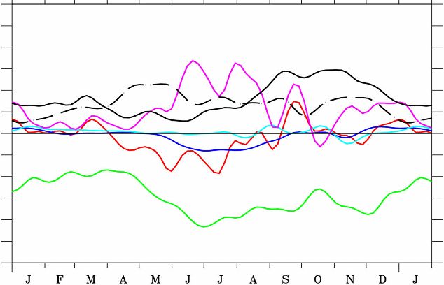
C06014                         PETER ET AL.: SEASONAL MIXED LAYER HEAT BUDGET                                         C06014

         Figure 1. Longitude-latitude plots of CLIPPER and T/P-ERS sea level anomalies: (a) CLIPPER
         standard deviation, (b) T/P standard deviation, (c) correlation, and (d) RMS difference (contours every
         1 cm, except for correlation, whose contour interval is 1). For this comparison we have linearly
         interpolated the model on the T/P-ERS grid.

The south east and north east trade winds converge in the        [21] Figures 4c and 4d depict the mean mixed layer depth,
ITCZ whose position in the northern hemisphere is one          in comparison with the dBM’s mixed layer depth climatol-
factor which explains the presence of cold water just south    ogy. The MLD is shallower in the eastern part of the basin:
of the equator, and warmer water north of it [see, e.g.,       10 m (both model and data), and deepens toward the west
Mitchell and Wallace, 1992]. The net heat flux is maximum      reaching 60 m in the observations but only 40 m in the
above the cold tongue (160 W m2), and minimum over the        model. This underestimation of the MLD is due to the
subtropical gyres (Figure 3a). The ECMWF global structure      combined effects of the absence of the very high-frequency
is in good agreement with other atmospheric heat flux data     wind stress forcing and of the insufficient vertical resolution
set. However, the zonally averaged net flux along the          which prevents the transmission of the wind stress energy to
equator from ECMWF (37 W m2) is underestimated when           the current shear and thus prevents the MLD from deepen-
compared to other data sets which are anyway not consistent    ing [Blanke and Delecluse, 1993]. Note that the high spatial
together (for instance, 47 W m2 for NCEP/NCAR Reanal-         resolution of the model allows the narrowness of the
ysis; 60 W m2 for UWM/COADS, and 89 W m2 for                 shallow mixed layer in the equatorial band to be repro-
SOC; for more details, see http://www-meom.hmg.inpg.fr/        duced. This is not visible with a weaker resolution such as
Web/Atlas/Flux/main.html). This is mainly due to too weak      in the work by dBM, but it is confirmed by close exami-
solar and latent heat fluxes [Yu et al., 2004].                nation of vertical profiles from hydrographic cruises such as
  [19] The modeled mean circulation in the upper ocean is      EQUALANT [Bourlès et al., 2002]. Despite a slight under-
realistic (Figure 3b), with the two branches of the westward   estimation of the modeled MLD in the west, the model
flowing South Equatorial Current (SEC) off the equator,        demonstrates a good ability to reproduce the mixed layer
separating into the southward flowing Brazil Current and       depth structure, a key feature for mixed layer heat budgets.
the northward flowing North Brazil Current. The latter feeds
the Guyana Current, and the eastward North Equatorial          3.2. Heat Budget
Countercurrent (NECC) which extends into the Guinea              [22] Figure 5 shows the mean 1997– 2000 state of the
Current in the GG. The subsurface circulation is validated     different tendency terms of equation (1). Over that time
and discussed in a specific study about the EUC [Arhan et      period, heat storage (left-hand side of equation (1)) is
al., 2006].                                                    observed to be close to zero.
  [20] The modeled spatial D20 distribution is in agreement      [23] The overall balance mainly results from cooling by
with TAOSTA observations [Vauclair and Du Penhoat,             vertical processes at the base of the ML (vertical advection,
2001] (Figures 4a and 4b). The zonal and meridional slopes     entrainment, vertical mixing), warming by atmospheric heat
of the thermocline are similar in the model and the data:      fluxes, and eddies, a picture very similar to Vialard et al.’s
along the equator, the thermocline deepens from 50 m in the    [2001] and Menkes et al.’s [2006] results in the Pacific
east to 120 m in the west in both data and model.              Ocean. The subsurface cooling is greater than 2.5C

                                                          4 of 16
C06014 PETER ET AL.: SEASONAL MIXED LAYER HEAT BUDGET C06014
Figure 2. Time-depth plots of (top) PIRATA moorings and (bottom) model temperature along the
equator at various longitudes: (a) 35W, (b) 23W, and (c) 10W (contours are 16C, 20C, and 24C).
The PIRATA data are filtered (5-day filtered).
Figure 3. Longitude-latitude plots of the 1997 – 2000 time average of (a) ECMWF total heat flux
(contours every 20 W m2) and ERS wind stress (102 N m2) and (b) CLIPPER mixed layer temperature
(contours every 0.5C) and CLIPPER currents (cm s1).
5 of 16C06014 PETER ET AL.: SEASONAL MIXED LAYER HEAT BUDGET C06014
Figure 4. Longitude-latitude plots of the 1997– 2000 time average of the 20C isotherm depth for
(a) CLIPPER and (b) TAOSTA (contours every 20 m) and of the mixed layer depth for (c) CLIPPER and
(d) de Boyer Montégut et al. [2004] (contours every 10 m). The criterion for the MLD is the depth at
which the density equals the surface density plus 0.05 kg m3.
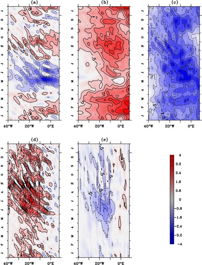
month1 south of the equator (0S – 2S), from 0W to strongest in the equatorial cold tongue: first, this is a
20W. Over the same area, warming by the atmospheric region of Ekman divergence and upwelling, with a thin
fluxes is about 1.5 to 2C month1. Warming by eddies thermocline and a strong vertical temperature gradient;
contribute to a rate of 1 to 1.5C month1 between 5W and secondly, the strong vertical shear between the surface
30W slightly north of the equator. The mean low-frequency SEC and the EUC results in strong vertical mixing.
meridional advection plays a minor role in the overall [26] The warming by the eddy term is located in the
balance and has mainly a cooling effect north of the equator region of most active TIWs [Chelton et al., 2000], and is
(0N – 2N) between 0 and 25W, with values locally similar in magnitude to the seasonal atmospheric heat flux.
reaching 1C month1. Finally, low-frequency zonal advec- The TIWs are tightly trapped within a narrow band north of
tion is a minor term only contributing to a warming patch of the equator, and reach their maximum at 15W, in agree-
0.5C month1 north of the equator (0N – 2N) in the ment with satellite observations [Legeckis and Reverdin,
western part of the GG (0 and 10W). 1987; Caltabiano et al., 2005]. In agreement with Jochum
[24] The atmospheric forcing term largely reflects the et al. [2004], the lateral diffusion is observed to be negli-
structure of the atmospheric net heat fluxes (Figures 5a gible when compared to TIWs.
and 3a). Its pattern is close to the total net heat flux, but [27] The low-frequency zonal advection heating pattern
depends also on the spatial structure of the mean MLD on the equator between 10W and 0 is due to the
(Figure 4c). A shallow MLD indeed concentrates the net westward current that brings warmer waters from the east
heat flux and increases the warming tendency close to the of the cold tongue (Figure 3b). Like the zonal advection,
equator. The strongest heating thus also corresponds to the mean advection by low-frequency meridional currents
the region of the strongest upwelling, enhancing the (Figure 4e) does not play a major role in the total
moderating effect of the atmospheric fluxes on the equa- balance. North and south of the cold tongue the merid-
torial upwelling. ional current flows poleward, in response to the equatorial
[25] The mean subsurface tendency term (Figure 5b) is divergence and thus brings colder water: this is a cooling
a cooling term all over the equatorial band. Like the term. This cooling is less effective in the south as the
atmospheric warming, the subsurface cooling is also the
6 of 16C06014 PETER ET AL.: SEASONAL MIXED LAYER HEAT BUDGET C06014
Figure 5. Longitude-latitude plots of the 1997 – 2000 time average of various contributors to the mixed
layer temperature: (a) atmospheric forcing, (b) tendencies due to vertical exchanges with the subsurface
ocean (sum of vertical advection, vertical diffusion at the base of the mixed layer, and entrainment),
(c) eddies (high-frequency horizontal advection plus lateral diffusion), (d) zonal advection by low-
frequency currents, (e) meridional advection by low-frequency currents (contours every 0.5C month1
between 2C month1 and 2C month1 and every 1C month1 after; the thick line is zero; and
dashed contours represent negative values).
meridional temperature gradient is weaker than in the decreases along the equator while zonal wind stress and
north. latent heat flux increase, driving the net heat loss close to its
minimum in May ( 20 W m2). The wind in the eastern
4. Seasonal Cycle part of the GG blows eastward in the GG (monsoon flux),
and strengthens between August and October. The net heat
4.1. Description and Validation
flux thus reaches its second maximum in late September
[28] Figure 6 shows the seasonal cycle of zonal wind (120 W m2). From September to December, the net heat
stress, net heat flux and thermocline depth. In March, the flux decreases to a second minimum (60 W m2). These
net flux (Figure 6a) reaches its first maximum in the central features are in agreement with Chang et al. [2000]. Figure 6c
part of the basin (110 W m2), when wind stresses are low shows the seasonal cycle of the modeled thermocline
(0.04 N m2). From March to May the net heat flux
7 of 16C06014 PETER ET AL.: SEASONAL MIXED LAYER HEAT BUDGET C06014
Figure 6. Longitude-time plots along the equator (2N–2S average) for the mean 1997– 2000 seasonal
cycle of (a) ECMWF net heat flux (contours every 30 W m2), (b) ERS zonal wind stress (contours every
102 N m1), and (c) model 20C isotherm depth (contours every 20 m).
depth which tightly responds to wind-forcing variability captured by the model, despite a lack of amplitude com-
(Figure 6b). In March the east-west thermocline slope is pared to TMI, in particular the cold tongue is not cold
slightly tilted and reverses east of 5W; this slope starts to enough in boreal summer.
increase in May and June during the intensification of the [30] Figure 7c depicts the seasonal variations of the
easterlies. As the easterlies relax in the center of the basin model MLD in comparison with dBM’s climatology
between June and October, the thermocline deepens at 0E. (Figure 7d). As the winds are more intense in the west,
The second intensification of the trade winds in November the mixed layer is deeper there than in the east. In March–
makes the thermocline shallow again in the whole basin. April, the wind stress is very weak and the ocean remains
These features are in good agreement with Hastenrath and highly stratified: the mixed layer is shallow (12 m from the
Merle [1987]. African coast to 30W in the model but deeper in the
[29] Figures 7a and 7b represent the SST seasonal cycle, observations). During May and June, the sudden increase
from the model and TMI. In March – April, the SST reaches of the easterly wind stresses very rapidly deepens the mixed
its maximum (28.5C in the model, 29.5C for TMI) in the layer in both model and observations. When wind stress
eastern part of the basin. Then the SST drops until August relaxes after November, the mixing reduces, the top of the
(23.5C in the model and 23C in observations) when the ocean stratifies and the ML thins. The MLD variations are
trade winds are strongest. Then, SST slowly rises from around 30 m in the west and 10 m in the east, representing a
August to March, except in boreal winter in the GG with a variation of 100% over the course of the season. Notice that,
short cold season in the model. This secondary cooling is even though the seasonal cycles of the thermocline and the
generally not captured well in most widely used climato- mixed layer depths are similar in the central and western
logical data because of their low resolution in space and tropical Atlantic, the cycles are not in phase in the east:
time. However, the 6-year PIRATA buoy observations when the MLD rapidly varies, the thermocline depth is at an
support the existence of this secondary seasonal cooling extremum, and vice versa (i.e., @ tMLD maximum when
(not shown). Notice that the seasonal warming and cooling @ tD20 = 0, and @ tD20 maximum when @ tMLD = 0).
are highly asymmetric at 10W, with the latter taking only [31] The seasonal cycles of the zonal current along the
3 months and the former taking 7 months. From the oceanic equator, for the simulation and the RMK product, are shown
point of view, this rapid cooling can be attributed to the in Figures 7e and 7f. In April, the westward flowing SEC
sudden and rapid intensification of the southerly winds in strengthens with the intensification of the trade winds
May – June in the GG, in link with the West African (Figure 6b), and reaches its maximum in June (0.5 m s1)
monsoon [Li and Philander, 1997; Xie and Carton, 2004]. with the right timing and location compared to RMK,
The main features of the SST seasonal cycle are well although with a weaker than observed intensity. During
8 of 16C06014 PETER ET AL.: SEASONAL MIXED LAYER HEAT BUDGET C06014
Figure 7. Same as Figure 6 but for SST from (a) CLIPPER and (b) TMI (contours every 1C), MLD
from (c) CLIPPER and (d) de Boyer Montégut et al. [2004] (contours every 10 m), and zonal current from
(e) CLIPPER and (f) Richardson and McKee [1984] (contours every 0.1 cm s1). The data of Richardson
and McKee [1984] are smoothed (1 longitude Hanning filter).
9 of 16C06014 PETER ET AL.: SEASONAL MIXED LAYER HEAT BUDGET C06014
the relaxation of the easterlies and the strengthening of the [36] From August to November, atmospheric forcing
westerlies (Figure 6b), the SEC drops and reverses from the significantly increases again (Figure 8b) because of higher
GG to 15W in September and October in agreement with solar heat flux and weaker easterlies in the center of the
RMK and other studies [Weisberg and Weingartner, 1988]. basin (Figure 6b). In association with the wind decrease, the
The second intensification of the trade winds in November drop in westward currents (Figure 7e), stratification
(Figure 6b) is associated with a second strengthening of the (Figure 6c) and shears (horizontal and vertical) in Septem-
SEC that reaches a maximum (0.4 m s1) in both model and ber and October reduce the effects of both subsurface
data. cooling and warming by TIWs. The situation is quite
different in the far western part of the basin where the
4.2. Seasonal Heat Budget easterlies (and the SEC) increase in July and August
4.2.1. Along the Equator (Figures 6b and 7e). This leads to an increase in subsurface
[32] This section first describes the heat balance in the cooling compared to the previous period, due to stronger
equatorial band (2N – 2S mean). The various tendency mixing at the base of the ML. The TIWs also remain intense
terms of the heat budget seasonal cycle (1997– 2000 mean) there. The warming by eddies and the subsurface cooling
are presented in Figure 8. partly compensate each other and the increase in surface net
[33] Heat storage along the equator is driven by the heat flux drives the observed rise of the SST. In the GG, the
cooling action of the subsurface term (Figure 8c), and the TIWs are almost nonexistent, so the heat storage is domi-
warming by both atmospheric forcing (Figure 8b) and nated by the surface warming and the subsurface cooling.
eddies (Figure 8d). Zonal and meridional advections by The atmospheric forcing is weak from August to November,
low-frequency currents are relatively weak except in boreal as the westward current decreases and even reverses in the
summer (Figure 8e), and compensate each other. For more GG. The decrease in stratification and in subsurface cool-
legibility, they are regrouped. There are four distinct periods ing, together with the increase of surface atmospheric
in the heat storage seasonal cycle (Figure 8a): (1) from forcing, leads to a warming of the sea surface (Figure 8a).
January to the end of March, the mixed layer warms slowly, Though partly balanced by the subsurface term and modu-
(2) in April, the cooling starts, and goes on until August, lated by TIWs in the western part of the basin, the increase
with a maximum cooling in May of around 5W, (3) the in solar radiation is the dominant factor that explains the
mixed layer is then heated again until December, (4) in warming from August to November (Figure 7a).
December, a second and weaker boreal winter cooling can [37] In boreal fall and winter, the atmospheric warming
be identified in the eastern part of the basin (Figure 7a). decreases in the GG during the winter monsoon because of
[34] Between January and March, as the ITCZ moves the associated high cloud coverage [Okumura and Xie,
close to the equator, winds and currents are weak (Figures 2005]. Only in the GG the decrease in solar flux, associated
6b and 7e); the contributions of the subsurface cooling term with the increase in subsurface cooling, allows the SST to
and the TIWs are thus weak, and the surface heating is the cool.
dominant term (Figure 8b) that drives the positive heat [38] The overall analysis explains why the SST seasonal
storage and the resulting SST warming with a maximum cycle is annual in the central and western parts of the basin,
SST at the end of March (Figure 7a). with a short intense cooling period between April and July
[35] The strong cooling between April and August is and a longer period of slight warming, and semiannual in
linked to both a clear decrease in the warming by atmo- the GG with a short second cooling period in December.
spheric forcing and an increase in the subsurface cooling, 4.2.2. Latitudinal Structure
but is moderated by warming by TIWs. In April and May, [39] To characterize latitudinal structure of the heat bud-
the easterlies suddenly strengthen at the equator, forcing a get, two longitudes were selected: 23W (representative of
strong SEC (Figures 6b and 7e). Atmospheric heat forcing western and central parts of the basin and location of
drops (Figure 6a) because of the decrease in solar heat flux PIRATA moorings) and 3E (eastern part of the basin and
and the increase in latent heat loss via evaporative cooling. location of repeated hydrographic sections).
Vertical diffusion cooling, induced by strong mixing pro- [40] At a first glance, Figure 9 shows that the heat storage
cesses, is enhanced. At that time, the currents are swift and evolution south of the equator and north of it is mainly
are prone to instability; they generate tropical instability governed by atmospheric forcing in the central part of the
waves in the center of the basin, that act to warm the basin (Figures 9a and 9b). North (4N – 8N) and south
equatorial band from 5W to 30W (Figure 8d). This (4S – 8S) of the equator, the subsurface term tends to cool
warming by TIWs is not strong enough to counteract the the mixed layer temperature except during the cold season
two previous effects, which result in a net heat loss and a when it tends to warm it at 23W because of the presence of
progressive SST decrease, reaching its minimum at the a barrier layer. Except in the northeastern part of the basin
beginning of August (Figure 7a). In the far western part where the eddies play a significant role in the temperature
of the basin, the increase in latent heat loss is enhanced by evolution (Figure 9c), this term is very small, like low-
higher wind stress (Figure 6b), the subsurface cooling is less frequency advections.
efficient as the thermocline remains deep, and the warming [41] As for the equatorial band, the seasonal cycle off
by the TIWs remains weak because the waves generated equator reveals four periods. In the central part of the basin
around 5W have not yet reached the western part of the (23W, Figures 9a and 9b) at the beginning of the year, from
basin; almost every term plays a role in the SST drop there. February to April, the SST is maximum north of the equator
East of 15W, TIWs play almost no role and vertical (29.5C, not shown). During this period, the vertical effects
diffusion cooling induced by strong mixing processes are close to zero, with a strong stratification, and the mixed
dominates over all terms. layer temperature cycle is entirely controlled by the net
10 of 16C06014 PETER ET AL.: SEASONAL MIXED LAYER HEAT BUDGET C06014
Figure 8. Longitude-time plots along the equator (2N – 2S average) of 1997– 2000 mean seasonal
cycles of (a) heat storage, (b) atmospheric forcing, (c) tendencies due to vertical exchanges with the
subsurface ocean (sum of vertical advection, vertical diffusion at the base of the mixed layer, and
entrainment), (d) eddies (high-frequency horizontal advection plus lateral diffusion), and (e) zonal and
meridional advections by low-frequency currents (contours every 0.5C month1 between 2C
month1 and 2C month1 and every 1C month1 after; the thick line is zero). All the trends are
smoothed with a 25-day Hanning filter.
11 of 16C06014 PETER ET AL.: SEASONAL MIXED LAYER HEAT BUDGET C06014
Figure 9. Time plots of 1997 – 2000 mean seasonal cycles, in C month1. Plots (left) at 23W:
(a) 4N–8N average and (b) 4S – 8S average and (right) at 3E: (c) 4N –8N average and (d) 4S – 8S
average. The red line is heat storage, the black line is atmospheric forcing, the green line is subsurface,
the purple line is horizontal advection by eddies, and the blue line is zonal and meridional advections by
low-frequency currents.
surface forcing. With the increase of the winds in April, the low-frequency advections. Contrary to what happens in the
atmospheric forcing decreases and the MLD deepens, in other locations, the eddies make an important contribution
May, and therefore SST also decreases. North of the to the heat budget, especially from April to October. In the
equator, the increasing heat flux provokes a second warm- southern part of the GG (Figure 9d), the mixed layer
ing in boreal fall, and a second cooling in December. South temperature cycle is dominated by the heat flux cycle.
of the equator, the overall trend cycle is annual and is driven
essentially by the atmospheric processes with a brief cold 5. Discussion
period which extends from April to August and a warming
tendency over the rest of the year. [43] We calculated a mixed layer heat budget in the
[42] East of 10W, the situation is different. In the equatorial Atlantic with a similar method as Vialard et al.
northern part of the GG, the seasonal cycle of the wind is [2001]. Our results in term of dominant processes are
more pronounced because of the African monsoon which comparable.
causes the trade winds to reverse in boreal summer, with a [44] In the present study, the different contributors to heat
semiannual component corresponding to the two rainy budget are found to be very similar to Jochum et al. [2005].
seasons on the African coast. The first takes place in boreal For instance, the explicit lateral diffusion is negligible when
summer, the second occurs in boreal winter. This semian- compared to TIWs, confirming that models resolving TIWs
nual signal is very pronounced as an overall trend, in scales are needed to accurately estimate heat budgets in the
atmospheric forcing, and in subsurface (Figure 9c). The tropical oceans. However, the mechanisms of equatorial
temperature in the ML is entirely driven by the semiannual zone warming by TIWs in the Pacific and Atlantic oceans,
atmospheric heat flux cycle, although its amplitude is and their effect on the mixed layer budget are the subject of
moderated by the cooling action of the subsurface processes, controversies. On one hand, Vialard et al. [2001] with a
and to a lesser extent by the nearly constant horizontal model in the Pacific, and Weisberg and Weingartner [1988]
12 of 16C06014 PETER ET AL.: SEASONAL MIXED LAYER HEAT BUDGET C06014
with observations in the Atlantic, show that TIWs warm the present study and the data in terms of signs, amplitude,
cold tongue through the transport of heat from the north to mean values, and latitudinal evolution. The major differ-
the cold tongue, to regulate the heat stored in the NECC. On ence between the two heat budgets concerns the process
the other hand, Jochum et al. [2005] claim that TIWs do not responsible of the cooling: subsurface term (entrainment +
heat from the equatorial cold tongue with heat advected vertical advection + vertical diffusion) in the present
from the warm pool, but draw their heat from the atmo- study and zonal advection by low-frequency currents of
sphere. First, Jochum et al. [2004] suggest, from a numer- FGCM. This difference may originate from the strong
ical experiment, that eddy-induced horizontal and vertical residue that is found in FGCM’s budget, especially at
fluxes almost compensate over a mixed layer of constant 10W, that may be due to an underestimation of the
depth (20 m), thus preventing TIWs from warming the vertical processes estimated from observations. Besides,
equatorial cold tongue. On the contrary, there is almost no the importance of the mean zonal advection in observa-
compensation when TIW-induced horizontal and vertical tions compared to our model may result from the scarcity
advections are computed (instead of flux divergences ap- of the observations, essentially based on drifters data that
proach which does not allow separating the influence of rapidly diverge from the equator.
mass convergence) over a time- and space-varying mixed [47] However, the model also has limitations, first the
layer (see Menkes et al. [2006] for a thorough discussion). relaxation term added to the ECMWF atmospheric heat
Second, in our model, a particle starting at the surface in the fluxes. Figures 10d, 10e, and 10f show the seasonal
equatorial upwelling is advected away to the north where it cycles of the relaxation term (in black dashed lines)
encounters the SST front and downwells, escaping from the and the total net heat flux (ECMWF + relaxation, in
direct atmospheric forcing while recirculating back to the black continuous lines). The relaxation term is always
equator and up in the equatorial waters. Furthermore, while positive, whatever the location, in agreement with the
a typical particle entrained in a TIW recirculates, a number previously discussed cold bias in the equatorial modeled
of particle from the NECC are entrained into passing SST. This term is necessary everywhere for the mean
vortices associated to the TIWs. These warm particle waters state, but important for the seasonal cycle only in the
actually do transport heat from the NECC warm waters to eastern part of the basin. It might account either for
the cold tongue (P. Dutrieux, personal communication, uncertainties in the ECMWF atmospheric heat fluxes or
2002). Thus, in our model configuration, there is a direct unresolved dynamics and thermodynamics in the present
oceanic heat transport from the NECC to the cold tongue. oceanic model. Comparisons with satellite or in situ data
Yet, it has been demonstrated in observations that the show that ECMWF net heat flux is too weak near the
atmosphere is structured at the TIW scales. It is thus likely equator. Comparison between PIRATA flux and ECMWF
that the atmosphere indeed retroacts on the ocean heat flux also reveals that the primary role of the relaxation
transport at the TIW scale. However, how this actually term is to bring the ECMWF flux nearer the observed
occurs is yet to be resolved and would need, from a flux. The relaxation term may account in particular for a
modeling point of view, the construction of a fully coupled possible bad representation of the cloudiness over the
ocean-atmosphere high-resolution model. GG. Furthermore, to illustrate uncertainties due to atmo-
[45] Comparisons with studies of the SST heat budgets spheric forcing, we have computed the same mixed layer
computed from observations [Merle, 1980; Weingartner heat budget with another configuration of OPA, ORCA05
and Weisberg, 1991] in the equatorial Atlantic give (see details of this configuration in work by de Boyer
qualitatively similar results despite different methodolo- Montégut et al. [2006]), which is forced in bulk formulae
gies. In particular, Weingartner and Weisberg [1991] for heat and salt fluxes. The results are presented on
explained the seasonal variations in SST by several Figure 10 (left). We observed that even though seasonal
different mechanisms, each operating at a different phase amplitudes are different (Figures 10a, 10b, and 10c), the
of the annual cycle: the rapid decrease in SST in boreal relative importances of the terms are the same
spring and the appearance of the cold tongue was (Figure 10g), which means that the overall heat balance
attributed primarily to upwelling-induced cooling by ver- is unchanged. This suggests that, in spite of the differ-
tical advection; they found an increase in the horizontal ences in spatial resolution and in the parameterization of
advection with the onset of the instability wave season lateral diffusion between the two simulations, our results
wherein a meridional Reynolds’ heat flux convergence are largely independent of the choice of a specific heat
resulted in increasing SST, which was then driven by flux data set. This important conclusion holds also for the
surface heat flux. These results are qualitatively (if not wind stress as demonstrated in the equatorial Pacific by
quantitatively) comparable to the present results. Cravatte et al. [2005]. Secondly, as shown in validation
[46] In a recent study, FGCM used in situ temperatures sections, the vertical structure is not exactly simulated by
from PIRATA moorings, near-surface drifting buoys, and CLIPPER with an underestimation of the MLD in the
a blended satellite – in situ SST product to calculate mixed western part of the basin, and a slightly too diffuse
layer temperature evolution in the tropical Atlantic Ocean. thermocline compared to in situ data. Even if the strat-
Minimum, maximum and mean of the different terms of ification underestimation leads to an augmentation of the
both heat budgets are presented in Figure 10 (left). The vertical diffusion coefficient (the current shear seems
seasonal evolution of the modeled trends (Figure 10, realistic), the too diffusive thermocline tends to underes-
right) can be compared to Figure 5 of FGCM. Except timate the vertical diffusion and the entrainment, by
for the contributions of the vertical cooling terms and the decreasing the temperature vertical gradient (equation (1)).
low-frequency advections, one can see on Figures 10a, This underestimation of the cooling should induce warmer
10b, and 10c the reasonable agreement between the SST than observed, which is not the case, suggesting that
13 of 16C06014 PETER ET AL.: SEASONAL MIXED LAYER HEAT BUDGET C06014
Figure 10. Heat budget annual tendencies (W m2) and mixed layer depth (m, in yellow) for CLIPPER
(left bars), ORCA05 (middle bars) and PIRATA (right bars) at (a) 35W –0N, (b) 23W – 0N, and
(c) 10W – 0N. The PIRATA heat budget values are from Foltz et al. [2003]. The bars represent
minimum, maximum (vertical bars), and mean (horizontal bars). Seasonal cycle of CLIPPER tendencies
around (d) 35W – 0N, (e) 23W – 0N, and (f) 10W – 0N, in W m2. (g) Relative contributions (%) of
the various terms for the total budget in CLIPPER (left bars), ORCA05 (middle bars), and PIRATA (right
bars). Heat storage is given in red, forcing is given in black (dashed line is the damping contribution),
subsurface is given in green, horizontal advection by eddies is given in purple, zonal advection by low-
frequency currents is given in dark blue, and meridional advection by low-frequency currents is given in
light blue.
there is not enough warming, from either surface heat contribution to the mixed layer temperature budget. Fi-
fluxes or TIWs. The too shallow MLD cannot explain nally, another source of uncertainties in our numerical
this surestimation: indeed, if the atmospheric heat fluxes approach is parameterization of the vertical and lateral
were integrated on a deeper layer, it would decrease their diffusion, which has been shown to be crucial for the
14 of 16C06014 PETER ET AL.: SEASONAL MIXED LAYER HEAT BUDGET C06014
variability in the Tropical Ocean [Blanke and Delecluse, pertinent contributions to these analyses. We would also like to thank
Marchus Jochum; an anonymous reviewer; and the editor, Raghu Murtu-
1993]. gudde, for their very useful comments and suggestions.
6. Summary References
Arhan, M., A. M. Treguier, B. Bourlès, and S. Michel (2006), Diagnosing
[48] In this study, the seasonal cycle of the equatorial the annual cycle of the Equatorial Undercurrent in the Atlantic Ocean
mixed layer heat budget is investigated using a numerical from a general circulation model, J. Phys. Oceanogr., in press.
simulation of the Tropical Atlantic. A high-resolution ocean Barnier, B., L. Siefridt, and P. Marchesiello (1995), Thermal forcing for a
global ocean circulation model using a three-year climatology of
general circulation model is used to diagnose the various ECMWF analyses, J. Mar. Syst., 6, 363 – 380.
contributions to a local and closed mixed layer heat budget. Blanke, B., and P. Delecluse (1993), Variability of the tropical Atlantic
The simulation reproduces reasonably well the main fea- Ocean simulated by a general circulation model with two different mixed
layer physics, J. Phys. Oceanogr., 23, 1363 – 1388.
tures of the circulation and thermal structure of the tropical Bourlès, B., M. D’Orgeville, G. Eldin, Y. Gouriou, R. Chuchla, Y. DuPenhoat,
Atlantic. The modeled closed mixed layer heat budget is and S. Arnault (2002), On the evolution of the thermocline and subthermo-
decomposed into six terms: the temperature evolution, the cline eastward currents in the equatorial Atlantic, Geophys. Res. Lett.,
atmospheric flux forcing, the vertical processes (sum of 29(16), 1785, doi:10.1029/2002GL015098.
Busalacchi, A. J., and J. Picaut (1983), Seasonal variability from a model of
vertical diffusion, vertical advection and entrainment), the tropical Atlantic Ocean, J. Phys. Oceanogr., 13, 1564 – 1588.
the eddies (regrouping the horizontal high-frequency Caltabiano, A. C. V., I. S. Robinson, and L. P. Pezzi (2005), Multi-year
(35 days). Unlike ture in the tropical Atlantic Ocean, J. Geophys. Res., 102, 27,813 –
several other studies, the SST equation is integrated over a 27,824.
Chang, P., R. Saravanan, L. Ji, and G. C. Hegerl (2000), The effect of local
time- and space-varying mixed layer. sea surface temperatures on atmospheric circulation over the tropical
[49] At a first order, the SST balance at the equator is Atlantic sector, J. Clim., 13, 2195 – 2216.
found to be the result of both cooling by subsurface Chelton, D. B., F. J. Wentz, C. L. Gentemann, R. A. de Szoeke, and M. G.
processes (through vertical mixing at the base of the mixed Schlax (2000), Satellite microwave SST observations of transequatorial
tropical instability waves, Geophys. Res. Lett., 27(9), 1239 – 1242.
layer, vertical advection and entrainment), and heating by Cravatte, S., C. E. Menkes, T. Gorgues, O. Aumont, and G. Madec (2005),
atmospheric net heat fluxes and eddies (mainly TIWs). The Sensitivity of the modeled dynamics and biogeochemistry of the equator-
cooling by subsurface processes is strongest in June – ial Pacific Ocean to wind forcing during the 1997 – 1999 ENSO, paper
presented at the 1st Alexander von Humboldt International Conference
August and December when the easterlies are strong. on the El Niño Phenomenon and its Global Impact, Eur. Geosci. Union,
Heating by the atmosphere is maximum in February – March Guayaquil, Ecuador, 16 – 20 May.
and September – October, whereas the eddies are most active de Boyer Montégut, C., G. Madec, A. S. Fischer, A. Lazar, and D. Iudicone
(2004), Mixed layer depth over the global ocean: An examination of
in boreal summer. On the other hand, horizontal advection profile data and a profile-based climatology, J. Geophys. Res., 109,
by low-frequency currents only plays a minor role in the C12003, doi:10.1029/2004JC002378.
heat budget. Off equator, the sea surface temperature de Boyer Montégut, C., J. Vialard, S. S. C. Shenoi, D. Shankar, F. Durand,
variability is mainly governed by atmospheric forcing all C. Ethé, and G. Madec (2006), Simulated seasonal and interannual varia-
bility of mixed layer heat budget in the northern Indian Ocean, J. Clim.,
year long, except in the northeastern part of the basin where in press.
strong eddies generated at the location of the thermal front Du Penhoat, Y., and A. M. Treguier (1985), The seasonal linear response of
significantly contribute to the heat budget in boreal summer. the tropical Atlantic Ocean, J. Phys. Oceanogr., 15, 316 – 329.
Duvel, J.-P., R. Roca, and J. Vialard (2004), Ocean mixed layer temperature
[50] Comparisons with previously published observational variations induced by intraseasonal convective perturbations over the
studies show relatively close conformity. However, this Indian Ocean, J. Atmos. Sci., 61, 1004 – 1023.
study reveals the major role played by the vertical Foltz, G. R., S. A. Grodsky, J. A. Carton, and M. J. McPhaden (2003),
Seasonal mixed layer heat budget of the tropical Atlantic Ocean, J. Geo-
exchanges at the base of the mixed layer that might be phys. Res., 108(C5), 3146, doi:10.1029/2002JC001584.
partly corresponding to the residue in heat budgets com- Fontaine, B., P. Roucou, and S. Trzaska (2003), Atmospheric water cycle
puted from observations. Experiment with higher-vertical and moisture fluxes in the West African monsoon: Mean annual cycles
resolution will be necessary to study the processes between and relationship using NCEP/NCAR reanalysis, Geophys. Res. Lett.,
30(3), 1117, doi:10.1029/2002GL015834.
the ML and the underlying thermocline. In particular, the Gibson, J. K., P. Kallberg, S. Uppala, A. Noumura, A. Hernandez, and
fact that the MLD and the thermocline variations are not in E. Serrano (1997), ERA description, ECMWF Re-anal. Proj. Rep. Ser. 1,
phase in the eastern part of the basin will be the subject of 77 pp., Eur. Cent. For Medium-Range Weather Forecasts, Reading, U. K.
Grima, N., A. Bentamy, K. Katsaros, Y. Quilfen, P. Delecluse, and C. Levy
further research. Moreover, the relaxation term, essential in (1999), Sensitivity of an oceanic general circulation model forced by
this oceanic model to simulate the mean state and the satellite wind stress fields, J. Geophys. Res., 104, 7967 – 7990.
seasonal cycle in the cold tongue region, highlights the Hastenrath, S., and J. Merle (1987), Annual cycle of subsurface thermal
structure in the tropical Atlantic Ocean, J. Phys. Oceanogr., 17, 1518 –
importance of improving the quality of the atmospheric heat 1538.
fluxes in the equatorial Atlantic. Cruises dedicated to study Houghton, R. W. (1989), Influence of local and remote wind forcing in the
of ocean-atmosphere interactions in the GG, as part of the Gulf of Guinea, J. Geophys. Res., 94, 4816 – 4828.
African Monsoon Multidisciplinary Analyses (AMMA) Houghton, R. W. (1991), The relationship of sea surface temperature to
thermocline depth at annual and interannual time scales in the tropical
program could be useful in this respect. Besides, more in Atlantic Ocean, J. Geophys. Res., 96, 15,173 – 15,185.
situ observations are needed to identify and quantify the Houghton, R. W., and C. Colin (1986), Thermal structure along 4W in the
vertical processes in the upper layer of equatorial oceans. Gulf of Guinea during 1983 – 1984, J. Geophys. Res., 91, 11,727 –
11,739.
Jochum, M., P. Malanotte-Rizzoli, and A. J. Busalacchi (2004), Tropical
[51] Acknowledgments. We would like to thank Anne-Marie Tregu- instability waves in the Atlantic Ocean, Ocean Modell., 7, 145 – 163.
ier (LPO, Brest, France) and Jean-Marc Molines (LEGI, Grenoble, France) Jochum, M., R. Murtugudde, R. Ferrari, and P. Malanotte-Rizzoli (2005),
for the CLIPPER runs. All the computations were performed on IDRIS The impact of horizontal resolution on the tropical heat budget in an
supercomputers. Special thanks are dedicated to Serena Illig, who brings Atlantic Ocean model, Clim, J., 18, 841 – 851.
15 of 16You can also read