Strong first order electroweak phase transition in 2HDM confronting future Z & Higgs factories - Inspire HEP
←
→
Page content transcription
If your browser does not render page correctly, please read the page content below
Published for SISSA by         Springer
                                                                   Received: January 14, 2021
                                                                    Accepted: March 18, 2021
                                                                     Published: April 22, 2021

Strong first order electroweak phase transition in
2HDM confronting future Z & Higgs factories

                                                                                                 JHEP04(2021)219
Wei Su,b Anthony G. Williamsb and Mengchao Zhanga,1
a
  Department of Physics and Siyuan Laboratory, Jinan University,
  Guangzhou 510632, P.R. China
b
  ARC Centre of Excellence for Dark Matter Particle Physics,
  Department of Physics, University of Adelaide,
  South Australia 5005, Australia
    E-mail: wei.su@adelaide.edu.au, anthony.williams@adelaide.edu.au,
    mczhang@jnu.edu.cn

Abstract: The electroweak phase transition can be made first order by extending the
Standard Model (SM) Higgs sector with extra scalars. The same new physics can explain
the matter-antimatter asymmetry of the universe by supplying an extra source of CP
violation and sphaleron processes. In this paper we study the existence of strong first
order electroweak phase transition (SFOEWPT) in the type-I and type-II two Higgs doublet
models (2HDM). We focus on how the SFOEWPT requirements constraint the spectrum
of non-SM Higgs. Through the parameter space scan, we find that SFOEWPT suggests
an upper limit on the masses of heavy Higgs mA/H/H ± , which is around 1 TeV. High
temperature expansion and Higgs vacuum uplifting is used for an analytical understanding
of our results. After taking into account the probe ability on SFOEWPT from theoretical
constraints, Higgs and Z-pole precision measurements up to the one-loop level at future
Higgs & Z factories, sizeable loop corrections require mA/H ± − mH ∈ (100, 250) GeV to
meet SFOEWPT condition for Type-II 2HDM, and |mA/H ± − mH | ∈ (100, 350) GeV or
|mA − mH/H ± | ∈ (100, 350) GeV for Type-I 2HDM.

Keywords: Supersymmetry Phenomenology

ArXiv ePrint: 2011.04540

    1
        Corresponding author

Open Access, c The Authors.
                                                     https://doi.org/10.1007/JHEP04(2021)219
Article funded by SCOAP3 .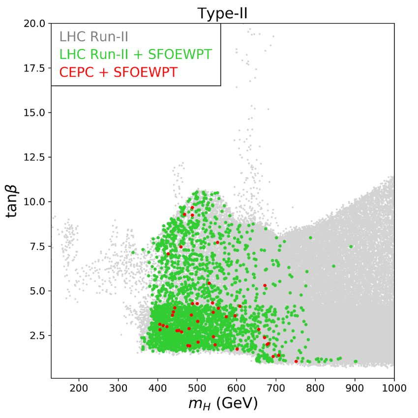
Contents

1 Introduction                                                                           1

2 The   electroweak phase transition in 2HDMs                                            3
  2.1   Two Higgs doublet models                                                         3
  2.2   Thermal effective potential                                                      4
  2.3   Numerical analysis method                                                        6

                                                                                              JHEP04(2021)219
3 Current and expected bounds                                                            7
  3.1 Theoretical constraints                                                            8
  3.2 Direct searches at LHC Run-II                                                      9
  3.3 Higgs and Z pole precision measurements                                           10
  3.4 Flavour constraints                                                               11

4 Study results                                                                         11
  4.1 The phase transition of 2HDM                                                      11
      4.1.1 High temperature expansion                                                  11
      4.1.2 Higgs vacuum uplifting                                                      13
  4.2 Case1: alignment limit with mA/H ± − mH = 200 GeV                                 17
  4.3 Case2: alignment limit with mA = mH ±                                             18
  4.4 Case3: alignment limit with mH = 700 GeV                                          19
  4.5 General results                                                                   20

5 Conclusion                                                                            24

1   Introduction

The discovery of the Higgs boson in 2012 completes the Standard Model (SM) [1, 2],
yet there remain observations that cannot be explained by it. One of the most famous
puzzles is the baryon asymmetry of the universe (BAU), which sees the visible matter in
our universe being dominated by baryons whilst the amount of anti-baryons is negligible.
Particle physics models that can successfully explain the BAU need to satisfy the three
Sakharov conditions [3]. The SM was once considered as a candidate model [4–6], since
baryon number conservation can be broken by an electroweak sphaleron process [4, 7, 8],
the CKM matrix provides CP violation, and the electroweak phase transition can induce a
departure from equilibrium if the Higgs boson is light enough. However, such an electroweak
baryogenesis (EWBG) mechanism in the SM framework turns out to fail, since the CP
violation present in the CKM matrix is too small [9] and the measured Higgs mass is
too heavy to trigger a strong first order electroweak phase transition (SFOEWPT) [10, 11].

                                          –1–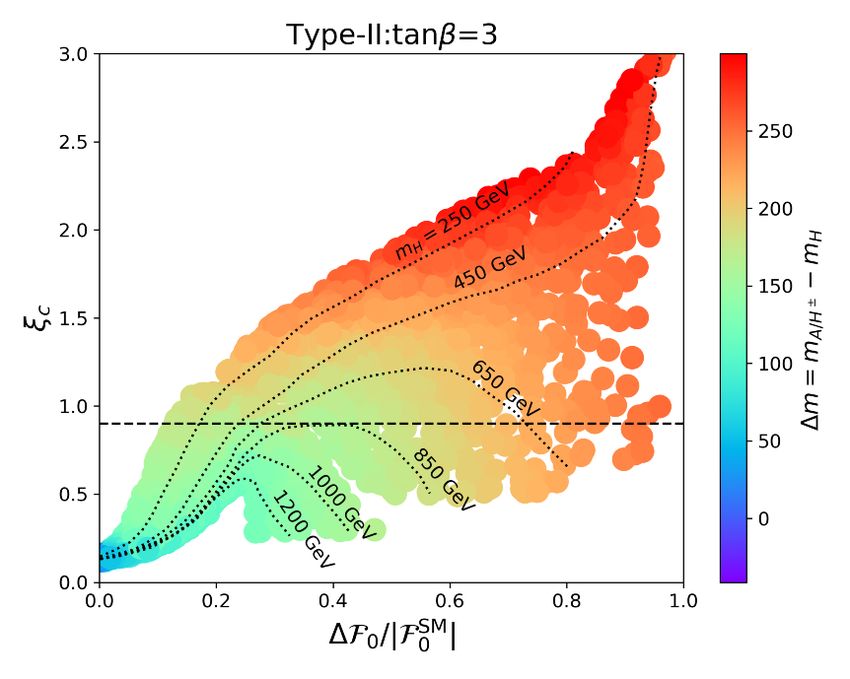
Thus for a successful baryogenesis, new physics beyond the SM (BSM) is required to supply
a new source of CP violation and a strong out-of-equilibrium process [12, 13]. In this work
we focus on the latter issue.
     In order to obtain a SFOEWPT, generally we need to extend the scalar sector of
the SM. Additional parameters in the scalar sector help to change the shape of Higgs
potential whilst leaving the Higgs vacuum expectation value (VEV) and the mass of Higgs
same. Simple SM extensions include the addition of a SU(2) singlet [14–31], an extra
doublet [32–69], an extra triplet [70–73], or extra higher dimensional operators [74–79].
Consideration of the hierarchy problem leads to further solutions such as embedding the
Higgs boson in a Composite Higgs model [80–82] or a supersymmetric model [83–98] to

                                                                                              JHEP04(2021)219
obtain a SFOEWPT. For a SFOEWPT in other models see [99–102]. In this work we
study the existence of a SFOEWPT in the type-I and type-II 2HDMs [103, 104]. These
models are attractive to study because the number of new parameters is relatively small.
In addition, both Higgs doublets in 2HDM models are charged under SU(2) × U(1) and
couple to SM fermions. This gives a greater range of observations that can probe the
models relative to models that are extended by SM singlet scalars.
     It is well known that, compared with other baryogenesis mechanisms, e.g. leptogene-
sis [105] or the Affleck-Dine mechanism [106], EWBG can be detected at the electroweak
scale and part of the parameter space can be covered by current or expected collider exper-
iments. In 2HDMs, in addition to the SM-like Higgs boson h, there are three non-SM Higgs
bosons, H/A/H ± . H/A/H ± couple to h and help to build an energy barrier between the
symmetric phase and the SU(2) × U(1) broken phase when the temperature of the universe
is around the electroweak scale. Then the phase transition, which is tunneling through
the energy barrier, can be first order and strong enough. In our study, we will show that,
in order for this strong first order phase transition to occur, the masses of H, A and H ±
bosons should all be smaller than about 1 TeV, and generally there needs to be a relatively
large mass splitting between the heavy Higgs bosons H, A and H ± .
     H, A, and H ± bosons with a mass lighter than 1 TeV can be directly produced at the
current LHC or future hadron colliders like the HE-LHC [107] or the SPPC [108, 109].
Channels like A/H → tt̄/bb̄/τ τ̄ , H ± → tb̄, or A → HZ [110–113] can be used for detection
or exclusion. Besides, through mixing and loop effects, the non-SM Higgs bosons also
change the predicted value of the oblique parameters S, T and U , and reduce the Higgs
couplings κi = gh ii2HDM /gh iiSM relative to the SM expectation. Future e+ e− colliders
like the ILC [114], FCC-ee [115, 116] and CEPC [108, 109] will copiously produce Z and
Higgs bosons, and thus those observables (especially the hZZ coupling) can be measured
with unprecedented precision. In this work, we perform a global fit to obtain the parameter
space of 2HDMs that simultaneously satisfies a SFOEWPT and the expected measurement
precision at future Z and Higgs factories.
     The structure of this paper is as follows. In section 2 we briefly introduce our 2HDM
models and calculation methods. In section 3 we list all relevant measurements that can be
used to constrain the parameter space of the type-I and type-II 2HDMs. Section 4 starts
with an analytic analysis which helps readers to understand the features of the electroweak
phase transition in 2HDMs. Then we study three simplified typical cases, and present the
most general scan result. We conclude this work in section 5.

                                          –2–
2 The electroweak phase transition in 2HDMs
2.1 Two Higgs doublet models
2HDMs without a Z2 symmetry generally induce dangerous flavour-violating couplings at
tree level. In this work we therefore consider 2HDMs with a soft Z2 symmetry breaking.
The tree-level scalar potential for a 2HDM can be written as:
λ1 † 2 λ 2 † 2
V 0 (Φ1 , Φ2 ) = m211 Φ†1 Φ1 + m222 Φ†2 Φ2 − m212 Φ†1 Φ2 + h.c. +
Φ Φ1 + Φ Φ2
2 1 2 2
λ 2
+ λ3 Φ†1 Φ1 Φ†2 Φ2 + λ4 Φ†1 Φ2 Φ†2 Φ1 + Φ†1 Φ2 + h.c. . (2.1)
5
JHEP04(2021)219
2
We consider a CP-conserving case, in which all mass parameters m2ij and quartic couplings
λi are real. After electroweak symmetry breaking (EWSB), the two SU(2)L Higgs doublets
Φi obtain VEVs vi , and they can be expanded in the component real scalar fields:
φ+ φ+
! !
1 2
Φ1 = √1 (v1 + h1 + ia1 )
, Φ2 = √1 (v2 + h2 + ia2 )
. (2.2)
2 2
with v12 + v22 ≡ v 2 ≈ (246 GeV)2 . We further define the ratio of VEVs as tan β ≡ v2 /v1 .
Two of the three m2ij can be replaced by other parameters by imposing conditions that
result from minimising the Higgs potential
v2 v12 v22
m211 = m212 − λ1 − (λ3 + λ4 + λ5 ) (2.3)
v1 2 2
v v 2 v12
1
m222 = m212 − 2 λ2 − (λ3 + λ4 + λ5 ). (2.4)
v2 2 2
Thus the squared mass matrices of the CP-even, CP-odd, and charged Higgs are:
!
m212 tan β + λ1 v12 −m212 + v1 v2 λ345
M2even = , (2.5)
−m212 + v1 v2 λ345 m212 / tan β + λ2 v22
!
tan β −1
M2odd = m212 − v 1 v 2 λ5 , (2.6)
−1 1/ tan β
1
!
tan β −1
M2charged = m212 − v1 v2 (λ4 + λ5 ) . (2.7)
2 −1 1/ tan β
Here λ345 ≡ λ3 + λ4 + λ5 . After diagonalization, the mass eigenstates are related to the
original fields by the rotation matrices:
! ! !
H cos α sin α h1
= , (2.8)
h − sin α cos α h2
! ! !
G0 cos β sin β a1
= , (2.9)
A − sin β cos β a2
φ±
! ! !
G± cos β sin β
= 1
(2.10)
H± − sin β cos β φ±
2
–3–We choose our input parameters to be:
cos(β − α) , tan β , m212 , mH , mA , mH ± . (2.11)
The mass of the SM-like Higgs boson mh is fixed to the current central measured value
125.09 GeV [117]. Then the λi can be re-expressed in terms of these input parameters.
Considering the theoretical constraints, including vacuum stability, perturbativity, and
unitarity, we introduce
m212
λv 2 ≡ m2H − , (2.12)
sin β cos β
JHEP04(2021)219
following the notation in [118]. Under the assumption of degenerate heavy Higgs √ masses
mH = mA = mH ± , there is no theoretical restriction on the tan β range when λv 2 = 0.
Type-I and Type-II 2HDMs have different Z2 parity assignments, and thus the cou-
plings between scalar and other particles have a different dependence on tan β and the
mixing angle α. The main difference between the Type I and Type II models is the de-
pendence of the couplings Af f¯ and Hf f¯ on the value of tan β. Couplings between A/H
and down-type fermions are suppressed by tan1 β in the Type I model, but are enhanced
by tan β in the Type II model. Thus the Type II model is generally more constrained by
experiments than the Type I model when tan β is large.
Here we need to emphasize that in the 2HDM we can set the mass of the non-SM Higgs
bosons A/H/H ± to an arbitrarily high scale. This is because of the presence of m211,12,22 ,
with m212 breaking Z2 symmetry in eq. (2.1). As can be seen from eq. (2.5) to eq. (2.7), the
squared masses of A/H/H ± arise from two types of contribution. One of them involves
terms of the form λi vj vk , which are bounded by perturbative unitarity and thus cannot be
too large. Upper-limits on these terms are roughly given by 4πv 2 ≈ (870 GeV)2 . Another
part of Higgs mass squares come from m212 (m211/22 are transformed through eq. (2.3) and
eq. (2.4)), and these terms can in principle be set to any value without violating theoretical
requirements. This makes the search for evidence of 2HDMs an endless game: you can never
completely falsify a New Physics model containing hypothetical particles which have no
upper limits on their mass.
However, in the following part of this work we will show that the requirement of a
SFOEWPT imposes upper limits on the masses of the A/H/H ± bosons, making it possible
to fully verify or falsify the idea of EWBG in 2HDMs in the near future.
2.2 Thermal effective potential
To study the phase transition in the early universe, we need to study the dependence of
the free energy density on the order parameter. In our case, the free energy density is the
thermal effective potential, and the order parameter is the homogeneous scalar VEV [119].
The thermal effective potential V (φ1 , φ2 , T ) at temperature T is composed of four parts:
V (φ1 , φ2 , T ) = V 0 (φ1 , φ2 ) + V CW (φ1 , φ2 ) + V CT (φ1 , φ2 ) + V T (φ1 , φ2 , T ). (2.13)
Here V 0 is the tree-level potential of our model, V CW is one-loop Coleman-Weinberg po-
tential, V CT is the counter term, and V T is the thermal correction.
–4–The tree-level potential V 0 (φ1 , φ2 ) is obtained by replacing the field operators Φ1 (x)
and Φ2 (x) in V 0 (Φ1 , Φ2 ) with the homogeneous field values √12 (0, φ1 )T and √12 (0, φ2 )T :
1 1 1 1 1
V 0 (φ1 , φ2 ) = m211 φ21 + m222 φ22 − m212 φ1 φ2 + λ1 φ41 + λ2 φ42 + λ345 φ21 φ22 . (2.14)
2 2 8 8 4
The one-loop Coleman-Weinberg potential V CW (φ1 , φ2 ) is given in the MS renormal-
ization scheme by [120]:
1 X m2i (φ1 , φ2 )
" #
V CW
(φ1 , φ2 ) = n i m4
(φ 1 , φ 2 ) ln − ci , (2.15)
64π 2 i i
µ2
JHEP04(2021)219
with the index i running over all massive particles. ni is the degrees of freedom of particle
i multiplied by (−1)2s (s is the spin of particle i), which is -12, -4, 6, 3, 2, 1, 2 and 1 for
quarks, leptons, W ± , Z, H ± , G0 , G± , and neutral scalars, respectively. ci is 56 for gauge
bosons, and 32 for other particles. m2i (φ1 , φ2 ) is the mass square of particle i with v1 and v2
in its expression being replaced by scalar field value φ1 and φ2 . The renormalization scale
µ is set to the zero temperature VEV v.
In eq. (2.11) we choose the scalar masses, mixing angle, and VEV ratio as our input
parameters. These parameters are considered as physical parameters. It means that the
VEVs are determined by the position of the minimum of the scalar potential, and squared
masses are given by the second order partial derivatives of the scalar potential with respect
to the scalar fields at the position of the minimum. Adding the Coleman-Weinberg correc-
tion will shift both the position of the minimum and the second order partial derivatives
of the tree-level potential.
Thus, in order to offset the modification, counter terms V CT (Φ1 , Φ2 ) need to be added
to the Lagrangian. For a CP-conserving 2HDM, V CT (Φ1 , Φ2 ) can be expressed as [52]:
δλ1 † 2 δλ2 † 2
V CT (Φ1 , Φ2 ) = δm211 Φ†1 Φ1 +δm222 Φ†2 Φ2 −δm212 Φ†1 Φ2 +h.c. +
Φ Φ1 + Φ Φ2
2 1 2 2
δλ 2
+δλ3 Φ†1 Φ1 Φ†2 Φ2 +δλ4 Φ†1 Φ2 Φ†2 Φ1 + Φ†1 Φ2 +h.c.
5
2
+δt1 φ1 +δt2 φ2 . (2.16)
Coefficients of counter terms, those δs, need to be fixed by “on-shell” conditions:
∂ψi V CT (Φ1 , Φ2 ) + V CW (Φ1 , Φ2 ) = 0
∂ψi ∂ψj V CT (Φ1 , Φ2 ) + V CW (Φ1 , Φ2 ) = 0, (2.17)
with ψi denoting all of the component scalar fields of Φ1 and Φ2 . These conditions are eval-
uated at the minimum of the scalar potential at zero temperature, where Φ1 = √12 (0, v1 )T
and Φ2 = √12 (0, v2 )T .1 After adding these counter terms, our input parameters can be
treated as physical parameters which are directly connected to observables.
1
Second order derivatives of V CW suffer from an infrared divergence originating from the massless
Goldstone boson when T = 0. This problem can be solved by introducing an IR cut-off mass [50].
–5–The thermal correction with ring resummation included is [121, 122]:
m2i (φ1 , φ2 ) m2j (φ1 , φ2 )
! !
T4 X T4 X
V (φ1 , φ2 , T ) = 2
T
ni J B + 2 nj J F (2.18)
2π i T2 2π j T2
!3/2 !3/2
T 4 X m̃2k (φ1 , φ2 , T ) m2k (φ1 , φ2 )
− nk − .
12π k T2 T2
Here, the index i denotes all gauge bosons and scalars, j denotes leptons and quarks, and
k denotes scalars and the longitudinal component of gauge bosons. The functions JB,F are
JHEP04(2021)219
two integrals which come from the scalar and fermion thermal corrections respectively:
Z ∞ h p i
JB (x) = dk k 2 ln 1 − exp(− k 2 + x) , (2.19)
0
Z ∞ h p i
JF (x) = dk k 2 ln 1 + exp(− k 2 + x) . (2.20)
0
The second line in (2.19) comes from ring resummation, which is used to avoid the in-
frared divergence that occurs when the scalar mass is much smaller than the temperature.
m̃2k (φ1 , φ2 , T ) is the thermal Debye mass, an expression for which can be found in the
literature [52, 122].
2.3 Numerical analysis method
An electroweak phase transition is considered to be strong enough only if the net baryon
number generated around the bubble wall is not significantly washed out by the sphaleron
process inside the bubble. This condition can be converted to the requirement on the value
of “wash out” parameter [123]:
vc
ξc ≡ > 0.9 (2.21)
Tc
Here Tc is the critical temperature
q where a second minimum of V (φ1 , φ2 , T ) that breaks
SU(2)×U(1) appears, and vc ≡ v12 (Tc ) + v22 (Tc ) reflects the scale of electroweak symmetry
breaking. Here v1 (Tc ) and v2 (Tc ) are the scalar field values which minimize V (φ1 , φ2 , Tc ).
The calculation of ξc suffers from theoretical uncertainties. The first problem is that the
ξc induced by V (φ1 , φ2 , T ) is not gauge independent by itself [124–126]. Missing higher-
order quantum corrections also induce a theoretical uncertainty [127]. For a concrete
model, one can use lattice simulations to obtain a reliable value of ξc [63], but such a non-
perturbative calculation is very computationally expensive. Being aware of the theoretical
uncertainty in the calculation of ξc , in this work we relax the criterion of a SFOEWPT to
ξc ≡ Tvcc > 0.9. On the other hand, for a first order phase transition to really happen in
the universe, the bubble nucleation rate should be larger than the Hubble expansion rate
at the nucleation temperature [33, 128]. This requirement can be considered as a further
constraint on the 2HDM parameter space. For a conservative estimate, in this work we
will not consider a requirement on the bubble nucleation rate.
–6–Analytically, Tc and vc can be obtained by solving the following equations:
V (0, 0, Tc ) = V (v1 (Tc ), v2 (Tc ), Tc ), (2.22)
∂
V (φi , φ2 , Tc ) = 0 (i = 1, 2), (2.23)
∂φ1 φ1 =v1 (Tc ),φ2 =v2 (Tc )
∂
V (φi , φ2 , Tc ) = 0 (i = 1, 2). (2.24)
∂φ1 φ1 =0,φ2 =0
To make (0, 0) and (v1 (Tc ), v2 (Tc )) as local minimum points of V (φi , φ2 , Tc ), Hessian matrix
of V (φi , φ2 , Tc ) at (0, 0) and (v1 (Tc ), v2 (Tc )) also need to be positive definite. However,
JHEP04(2021)219
due to the complicated form of V (φ1 , φ2 , T ), solving these equations analytically is quite
difficult. Instead, one can search for the critical temperature using a numerical method.
There are already public packages which can be used for numerical thermal phase transition
analysis, such as CosmoTransitions [129], BSMPT [61], and PhaseTracer [130]. We choose
BSMPT for our numerical analysis, since the 2HDM has been implemented in BSMPT as a
benchmark model, and BSMPT is written in C++ which helps to save numerical calculation
time. In BSMPT, the search for Tc is started from a high temperature (the default value
is 300 GeV), where the minimum position of V (φ1 , φ2 , T ) is (0, 0). Then BSMPT traces
the minimum position of V (φ1 , φ2 , T ) with decreasing temperature. If BSMPT detects a
minimum position jumping (0, 0) ⇒ (v1 (T 0 ), v2 (T 0 )) at a certain temperature T 0 , the search
stops and the output T 0 is the desired critical temperature Tc .
The full thermal phase transition history of the 2HDM could be complicated [59]. Mul-
tiple phase transition processes are possible. For baryogenesis, however, only the phase
transition that transfers (0, 0) ⇒ (v1 (T ), v2 (T )) is relevant. This is because a success-
ful baryogenesis requires the sphaleron rate to be very fast outside the bubble wall, i.e.
ΓSph ∼ (αW T )4 . While in the electroweak symmetry breaking phase, the sphaleron rate
will be strongly suppressed as ΓSph ∝ exp (−ESph (Tc )/Tc ). Here the sphaleron energy
ESph (Tc ) ∼ 10TeV× vvc . Thus another phase transition (v1 (T 00 ), v2 (T 00 )) ⇒ (w1 (T 00 ), w2 (T 00 ))
has nothing to do with baryogenesis, because the sphaleron rate outside the bubble will
be too low to generate baryon number.2 We will therefore not take this kind of phase
transition into account in this work.
3 Current and expected bounds
2HDMs are constrained by various theoretical considerations and experimental measure-
ments, such as vacuum stability, perturbativity and unitarity, as well as heavy flavor ob-
servations [131], electroweak precision measurements, and LHC Higgs measurements and
non-SM Higgs searches [132]. We briefly summarize below the constraints we adopt in the
following sections.
2 00 00 00 00
pspeaking, phase transition (v1 (T ), v2 (T )) ⇒ (w1 (T ), w2 (T )) may produce enough baryon
Strictly
2 00 2 00
number if v1 (T ) + v2 (T ) is very small and this phase transition is strong first order. But the possibility
to obtain such a parameter point is very low in a random scan. So we ignore this case.
–7–Theoretical Constraints: tanβ=3 Theoretical Constraints: λv2 =0 Theoretical Constraints
500 20 20
cos(β-α)=0.0
cos(β-α)=0.0
10 10
co mH =700 GeV
s(β
400 - α) ΔmA =ΔmC
=- 5
0.0
5 2
Δm=mAH± -mH (GeV)
co
λv 2 s(β 2
300 =0 -α
(Ge 2 )=
V 2) -0 0
.00
tanβ
tanβ
λv 2 5 1 230 200 100
=1
50 2
λv 2 (Ge 1
=20 V 2)
200 02 05 0.5
(Ge
V 2) 0.0
)=
0.5 -α
s(β
λv 2=
220 2 co
(GeV 2 0.2
)
100 .02
) =0
λv 2=230 2 (Ge 0.2 -α 0.1
V 2) s(β
co
0 0.1
200 400 600 800 1000 200 400 600 800 1000 -1252 0 2002 3002 4002 5002 6002
mH (GeV) mH =mAH± -200 (GeV) λv2 =mH2 -m12 2 /(sβ cβ ) (GeV2 )
JHEP04(2021)219
Figure 1. The impact of theoretical constraints in the mH − ∆m (left), mH − tan β (mid-
dle), λv 2 − tan β (right) planes. In the left panel,
√ the allowed region is under the lines with
tan β = 3, cos(β − α) = 0. In the middle panel, λv = 0 GeV, and the allowed region is to the left
2
of the corresponding lines. In the right panel, mH is fixed at 700 GeV, and the allowed region is
inside of the boundary line. See text for full details.
3.1 Theoretical constraints
• Vacuum stability.
In order to make the vacuum stable, the scalar potential should be bounded from
below [133–136]:
λ1 > 0 , λ2 > 0 , λ3 > − λ1 λ2 , λ3 + λ4 − |λ5 | > − λ1 λ2 (3.1)
p p
• Perturbativity and unitarity.
We adopt a general perturbativity condition of |λi | ≤ 4π, and for the unitarity
bound [137–141]:
q
3(λ1 + λ2 ) ± 9(λ1 − λ2 )2 + 4(2λ3 + λ4 )2 < 16π , (3.2)
q
(λ1 + λ2 ) ± (λ1 − λ2 )2 + 4λ24 < 16π , (3.3)
q
(λ1 + λ2 ) ± (λ1 − λ2 )2 + 4λ25 < 16π , (3.4)
|λ3 + 2λ4 ± 3λ5 | < 8π , |λ3 ± λ4 | < 8π , |λ3 ± λ5 | < 8π . (3.5)
To provide some general insights into the impact of these theoretical constraints, we
show in figure 1 the allowed regions in the mH − ∆m (left), mH − tan β (middle), and
λv 2 −tan β (right) planes, for various fixed values of the other
√ parameters. In the left panel,
we take tan β = 3, cos(β−α) = 0, fixing mA = mH ± . Here λv 2 = 0, 150, 300, 220, 230 GeV
are represented by the red, blue, green, purple, and orange lines, and the region under
the lines is allowed by the theoretical constraints. Generally, a larger heavy √ Higgs mass
mH corresponds to a smaller allowed √ mass splitting ∆m for any specific λv 2 . The al-
lowed
√ ∆m also gets smaller when λv gets larger, and here there is no region left for
2
λv > 232 GeV.
2
–8–√
In the middle panel with λv 2 = 0 GeV, we explore the effect of the parameter
cos(β − α). Here, based on the allowed | cos(β − α)| at the current LHC Run-II [142],
we take cos(β − α) = ±0.005 (dashed lines), and cos(β − α) = ±0.02 (solid lines) and
show the allowed region, which is to the left of the corresponding lines. We fix the mass
splitting ∆m = mA/H ± − mH = 200 GeV.3 Under cos(β − α) = 0, mH < 820 GeV is
allowed, independently of tan β. If cos(β − α) 6= 0, such as the 0.005 region shown by the
dashed lines, the allowed regions are reduced. As discussed in [118], the allowed regions
for opposite-sign cos(β − α) are symmetric around the line tan β = 1.
In the right panel, mH is fixed at 700 GeV, and ∆m = mA/H ± − mH = 0, 100, 200 and
230 are shown. The allowed region is inside of the boundary line. Larger√∆m leads to a
JHEP04(2021)219
smaller allowed λv 2 range, and ∆m > 230 GeV is no longer allowed. For λv 2 = 0, there
is no restriction on tan β.
3.2 Direct searches at LHC Run-II
We take into account the latest heavy Higgs searches at LHC Run-II, including
A/H → µµ [143, 144], A/H → bb [145, 146], A/H → τ τ [147–149], A/H → γγ [150–154],
A/H → tt [155], H → ZZ [156, 157], H → W W [158, 159], A → hZ → bb`` [160–163],
A → hZ → τ τ `` [162, 164, 165], H → hh [166–169], and A/H → HZ/AZ [170, 171]. To
investigate the impact on the 2HDM parameter space of the published null results in these
searches, we take the cross section times branching fraction limits, σ × BR, from the LHC
studies and reinterpret them for our 2HDM model points using the SusHi package [172] to
calculate the production cross-section at NNLO level, and the 2HDMC [173] code for Higgs
decay branching fractions at tree level.
As a first example, taking the benchmark point cos(β − α) = 0, m212 = m2H cos β sin β
and mA = mH + = mH + 200 GeV, we show the current collider limits in the mH − tan β
plane in figure 2, for both the Type I and Type II models. The various channels include
H/A → bb (red), H/A → τ τ (dotted orange), H/A → µµ (dot-dashed cyan), H/A → γγ
(dashed brown), H/A → tt (dot-dashed magenta) and 4t production (dashed purple), as
well as the exotic decay channel A → HZ (blue). Other decays such as A → Zh and
H → hh will only contribute if cos(β − α) deviates from zero at tree level [174].
For the Type-I model (left panel of figure 2), the exotic decay A → HZ channel cov-
ers mH < 2mt , tan β < 5 totally, and can reach to tan β = 10. Top quarks searches,
4t + A/H → tt, cover mH < 800 GeV for tan β < 0.3, and mH < 650 GeV for tan β < 1.1
A/H → τ τ, γγ then exclude the region m < 350 GeV, tan β < 1 Generally because of the
cot β-enhanced Yukawa coupling in Type-I model, only the small tan β region can be ex-
plored [132]. In the Type-II 2HDM (right panel), the top quark and H/A → γγ constraints
are similar to those for the Type-I model, while the fermionic decays A/H → bb, τ τ, µµ
could exclude mH to 800 GeV when tan β > 10 generally. Since the Hbb, and Hτ τ cou-
plings are tan β-enhanced, the A → HZ decay contributes a lot at medium and large tan β
regions, tan β > 0.5, mH < 2mt and tan β > 15, mH < 600 GeV Thus mH < 2mt is
totally excluded by all channels together in Type-II model, and only 1.5 < tan β < 10
is allowed for mH < 650 GeV, which is important for our later study of the electroweak
phase transition.
3
In our notation, when we use mA/H ± , it indicates mA = mH ± .
–9–50
Type-I: cos( ) = 0, mA = mH + 200 GeV 50
Type-II: cos( ) = 0, mA = mH + 200 GeV
A HZ
A/H bb
10 10 A/H
A
H/A
HZ
5 5
H/A
A/H tt A/H tt
tan
tan
1 1
0.5 0.5
H/A
H/A
JHEP04(2021)219
4t 4t
0.1 0.1
100 300 500 700 100 300 500 700
mH (GeV) mH (GeV)
Figure 2. Direct search constraints for the heavy Higgs mass spectrum mA = mH ± = mH +
200 GeV. We show the 95% C.L. exclusion region in the mH − tan β plane for the Type-I 2HDM
(left) and Type-II 2HDM (right) with cos(β − α) = 0. The various heavy Higgs decays include
i) the conventional search results on H/A → bb (red), H/A → τ τ (dotted orange), H/A → µµ
(dot-dashed cyan), H/A → γγ (dashed brown), H/A → tt (dot-dashed magenta) and 4t production
(dashed purple), and ii) exotic decay channels A → HZ (blue). Other considered decays such as
A → Zh, H → hh are not relevant since their couplings are proportional to cos(β − α).
3.3 Higgs and Z pole precision measurements
The SM has been tested with high precision via observables measured at the Z-pole from
LEP-I [175] and the LHC [176]. Future lepton colliders will further improve the precision
of measurements in the Higgs sector, and we therefore include hypothetical future lepton
collider results in our study. In ref. [177], it was shown that the precision reached by several
future e+ e− machines, including the CEPC program with an integrated luminosity of 5.6
ab−1 [108, 109], the FCC-ee program with 5 ab−1 of integrated luminosity [115, 116], and
the ILC with various center-of-mass energies [114], is similar. Thus, following the approach
adopted in refs. [177, 178], we will explore the CEPC proposals in detail.
In our analyses, we take the S, T, U data at 95% Confidence Level (C.L.) from table 2
of ref. [177], and the Higgs precision measurements from table 3 in the same reference. We
use a χ2 profile-likelihood fit,
Z H
(µ2HDM i )
− µobs 2
χ2 = (Xi − X̂i )(σ 2 )−1
ij (Xj − X̂j ) + (3.6)
X X
i
2
,
ij i
σ µi
with Xi = (∆S , ∆T , ∆U )2HDM being the 2HDM predicted values, and X̂i = (∆S, ∆T, ∆U )
being the current best-fit central value for current measurements, and 0 for future measure-
ments at the first term for Z sector. The σij are the error matrix, σij
2 ≡ σ ρ σ with σ and
i ij j i
correlation matrix ρij given in [177]. For the second term about Higgs sector, Higgs preci-
sion measurements are used to perform global fit with µ2HDM
i = (σi ×Bri )2HDM /(σi ×Bri )SM
– 10 –is the signal strength for various Higgs search channels, σµi is the estimated error for each
process. The studies [177, 178] show that one-loop level electroweak corrections to SM
Higgs couplings have probe ability to heavy Higgs with Higgs precision measurements, and
thus our study of
For future colliders, the various µobs
i are set to be unity in the current analyses, as-
suming no deviations from the SM observables.
In the following analyses, the overall χ2 is calculated, and use to determine the allowed
parameter region at the 95% C.L. For the one-, and two-parameter fits, the corresponding
∆χ2 = χ2 − χ2min values at the 95% C.L. are 3.84, and 5.99 respectively.
JHEP04(2021)219
3.4 Flavour constraints
The charged Higgs H ± boson couples to up and down type fermions, and thus observations
from flavor physics put strong bounds on its mass and couplings [179]. Among various
flavor observations, measurements related to B physics provide the most stringent limits
on tan β and mH ± . For example, mH ± < 580 GeV in the Type-II 2HDM has been excluded
by the measurement of BR(B → Xs γ) [180]. ∆MBs and BR(Bs → µ+ µ− ) further exclude
mH ± < 1 TeV in the Type-II 2HDM when tan β < 0.7. The region with tan β < 1 and
mH ± < 1 TeV in the Type-I 2HDM has been excluded by B → Xs γ [180]. In our study,
we take these constraints into account.
4 Study results
Based on the diverse constraints above, in this section we will discuss their effects on the
SFOEWPT in Type-I and Type-II 2HDMs.
4.1 The phase transition of 2HDM
To get a better understanding of the electroweak phase transition in 2HDMs, we will first
discuss it in the context of some approximate or limiting cases, focusing on the relationship
between the phase transition and the Higgs vacuum uplifting. Then we will consider several
benchmark cases, varying one or two parameters to dig into the effects of constraints as
well as features of the Higgs potential. Our general results will follow these specific cases.
4.1.1 High temperature expansion
Due to the complicated form of the thermal effective potential eq. (2.13) and its intricate
thermal evolution history, it is difficult to tell whether a specific point can successfully
trigger a SFOEWPT in the early universe through a simple formula or argument. To
simplify the analysis of the phase transition, people generally use a high temperature
expansion, limited to the leading terms of the thermal correction functions JB and JF .
Then the thermal effective potential can be simplified to a polynomial function of the
Higgs field value:
λ̃
V (φh , T ) ≈ (DT 2 − µ2 )φ2h − ET φ3h + φ4h (4.1)
4
– 11 –Here φh ≡ cos βφ1 + sin βφ2 is the scalar field that breaks the SU(2) × U(1) symmetry
at zero temperature. Due to the simple form of eq. (4.1), we can use the minimization
condition and V (0, Tc ) = V (vc , Tc ) to directly calculate the wash-out parameter:
vc 2E
ξc ≡ ≈ (4.2)
Tc λ̃
At tree-level, the coefficients µ2 and λ̃ in eq. (4.1) are:
1 m2
µ2 = m2h , λ̃ = h2 (4.3)
4 2v
JHEP04(2021)219
The coefficients D and E are induced from the leading thermal corrections:
m2 (φh ) 1 1
!
T4 π2T 4
JB ≈− + T 2 m2 (φh ) − T (m2 (φh ))3/2 + · · · (4.4)
2π 2 T2 90 24 12π
m2 (φh ) 7 π2T 4 1
!
T4
JF ≈+ − T 2 m2 (φh ) + · · · (4.5)
2π 2 T2 8 90 48
Here m2 (φh ) is the mass square of a massive particle with v 2 in it being replaced by φ2h
m2
(For example, m2W (φh ) = vW
2 φh ). Considering the most massive particles in the 2HDM,
2
D and E can be expressed as:
1
" #
m2 m2Z m2h m2t m2H − M 2 m2A − M 2 m2H ± − M 2
D= 6 W + 3 + + 6 + + + 2 (4.6)
24 v2 v2 v2 v2 v2 v2 v2
1
" #
m3 m3 m3
E= 6 W + 3 3Z + 3h + E(H/A/H ± )
12π v 3 v v
In the expression for E, the term E(H/A/H ± ) denotes the contributions from the non-SM
Higgs bosons. We cannot explicitly write out the expression for E(H/A/H ± ) because, as we
said in section 2.1, the mass of the H/A/H ± bosons come from two sources. Schematically,
the φh -dependent non-SM Higgs squared masses can be expressed as:
m2α (φh ) = M 2 + λα φ2h (4.7)
m2
cos β is the scale at which the Z2 symmetry is broken. α can be A, H, or
Here M 2 = sin β 12
H , and λα is a linear combination of the λi (i = 1, 2, 3, 4, 5) parameters. In the alignment
±
limit cos(β − α) = 0, the expressions for λα are:
λH = (λ1 + λ2 − 2λ345 )(sin2 β cos2 β) , (4.8)
λA = −λ5 , (4.9)
1
λH ± = − (λ4 + λ5 ) (4.10)
2
So the non-SM Higgs bosons provide a term in V (φh , T ) which is not exactly propor-
tional to φ3h :
1 1
− T (m2α (φh ))3/2 = − T (M 2 + λα φ2h )3/2 (4.11)
12π 12π
– 12 –We can simplify the above expression in two limiting cases:
T 3/2 3 2 2
− 12π
1 λα φh , M
λα φ h
− T (M + λα φh ) ≈
2 2 3/2 2 (4.12)
12π − T M 3 1 + 3 λα φ2h , M 2
λα φ2
12π 2 M h
And so in these two limiting cases:
1 m3α
(
3/2
1
12π λα = 12π v 3 , M 2
λα φ2h
E(α) ≈ (4.13)
0, M 2
λα φ2h
JHEP04(2021)219
The above expression needs to be multiplied by 2 if α is H ± .
Although expression (4.13) is obtained in a limiting case, it helps us to understand
which of the input parameters are particularly relevant for a SPOEWPT. When the non-
SM Higgs masses are dominated by M 2 , the spectrum tends to be degenerate, and the phase
transition strength tends to be reduced as the non-SM Higgs boson masses increase. When
the non-SM Higgs masses are dominated by λα v 2 , the spectrum tends to be split, and the
phase transition strength tends to be increased as the non-SM Higgs boson masses increase.
4.1.2 Higgs vacuum uplifting
Another method that can help us to understand which parameters are important for
SFOEWPT, is to calculate the depth of the zero temperature Higgs potential [55]. For
a shallow Higgs potential, it is easier to develop an energy barrier between the symmetric
phase and the broken phase than for a deep Higgs potential, when the temperature is high.
Thus generally speaking, there is an inverse relation between the phase transition strength
and the depth of the vacuum energy. We follow the notation at ref. [55] and define the SM
vacuum energy density as F0SM . The value of F0SM is about −1.25 × 10⁸ GeV4 . The vacuum
energy density of the 2HDM is denoted by F0 . We can further define a dimensionless
parameter:
F0 − F0SM
∆F0 /|F0SM | ≡ (4.14)
|F0SM |
∆F0 /|F0SM | > 0 means that the 2HDM vacuum energy is uplifted from the SM value, whilst
∆F0 /|F0SM | cannot exceed 1, otherwise the zero temperature vacuum will be unstable.
The numerical results in [55] show a positive correlation between ξc and the parameter
∆F0 /|F0SM |. However, we find that the relationship is only valid for mH ≤ 500 GeV, the
range ref. [55] explored, and the parameters may become negatively-correlated for large
mH . To illustrate this, here we refine their analysis by considering a benchmark case:
tan β = 3.0, cos(β − α) = 0, mH ∈ (200, 1000) GeV , (4.15)
√
λv 2 = 0, ∆m = mA/H ± − mH = 200 GeV.
m2
All parameters are fixed except mH , and λv 2 = m2H − sin β 12
cos β = 0 (to meet the theoretical
constraints, as in the right panel of figure 1).
– 13 –Type-II Higgs potentia: T = 0 Type-II: cos(β-α)=0, tanβ=3
0.7 1.4
1 × 10⁸ mH = 800 (GeV)
mH = 600 (GeV)
0.6 1.2
mH = 400 (GeV)
5 × 10⁷ mH = 200 (GeV) 0.5 1.
V(ϕh ) (GeV4 )
Δℱ0 /|ℱ0 SM |
SM
0.4 0.8
ξ
0
0.3 0.6
7
-5 × 10 0.2 0.4
0.1 0.2
-1 × 10⁸
0 0
JHEP04(2021)219
0 100 200 300 400 200 300 400 500 600 700
ϕh (GeV) mH (=mAH± -200) (GeV)
Figure 3. Zero temperature Higgs potential and its connection with the electroweak phase tran-
sition. (left): the zero temperature Higgs potential along the φh ≡ cos βφ1 + sin βφ2 direction
with different mH . (right): vacuum energy uplifting ∆F0 /|F0SM | and wash-out parameter ξc as
functions of mH .
The one-loop level Higgs vacuum uplifting in the alignment limit cos(β − α) = 0 has
been given in ref. [55]:
1 3 1 4mA mH m2H ±
" " #!
2
∆F0 = m2
− 2M 2
+ log
64π 2 h
2 2
2
m2h − 2M 2
1 4
#
+ mA + m4H + 2m4H ± + m2h − 2M 2 m2A + m2H + 2m2H ± (4.16)
2
To illustrate the idea underlying Higgs vacuum uplifting, here we display the whole
shape of the zero temperature Higgs potential. In the left panel of figure 3, we present
the zero temperature Higgs potential along the φh ≡ cos βφ1 + sin βφ2 direction, with
mH = 200, 400, 600, 800 GeV represented by red, orange, green and blue lines respectively.
The SM Higgs potential is also shown with black dashed line for comparison. It is clear
that as mH increases, the height of the minimum point of the Higgs potential continues
to rise, and the shape of the Higgs potential becomes shallower. For large mH , F0 > 0,
generating an unstable vacuum. Thus for a stable vacuum mH cannot be too large.
To find the relationship between ξc and ∆F0 /|F0SM |, in the right panel of figure 3 we
present both ∆F0 /|F0SM | and ξc as functions of mH . In the plot, the left y axis is for
∆F0 /|F0SM | with the red dashed line representing the relationship with mH . While ξc , the
right y axis, is shown by the solid green line. Here ξc is calculated numerically from the
package BSMPT.
As the red dashed line, it is clear that there is a linear relationship between ∆F0 /|F0SM |
and mH , similar as the left panel. But as the green line shows, ξc is not monotonically
dependent on mH and gets the maximum value around mH = 500 GeV. This result can be
understood by our high temperature expansion analysis. Generally as mH , equal to M 2
in our scenario to meet theoretical constraints, becomes too large, the non-SM Higgs mass
– 14 –is dominated by M 2 and E(H/A/H ± ) get smaller as eq. (4.13). Thus the phase transition
strength becomes weaker as mH increases from eq. (4.6) and eq. (4.1).
Since ∆F0 /|F0SM | always gets larger when mH grows, while ξc gets larger at first
(mH < 500 GeV here), and then gets smaller, we can conclude ∆F0 /|F0SM | is not mono-
tonically correlated with ξc . This conclusion is different to the previous study [46].
In order to get a more robust relationship between ∆F0 /|F0SM | and ξc , as well as
exploring the mass splitting effects ∆m = mA/H ± − mH , we extend the benchmark case
by including different mass splittings between the non-SM Higgs bosons:
tan β = 3.0, cos(β − α) = 0, mH ∈ (200, 1000) GeV , (4.17)
√
JHEP04(2021)219
λv 2 = 0, ∆m = mA/H ± − mH ∈ (0, 300) GeV.
The reason for us to consider different mass splittings is that the mass splitting between
different non-SM Higgs bosons is roughly proportional to the size of the couplings λi .
Generally speaking, the greater the couplings λi , the easier it is for the non-SM Higgs
bosons to change the shape of the Higgs thermal potential from eq. (4.13) and eq. (4.18).
However, as can be seen from eq. (4.16), a large mass splitting tends to be more limited
by vacuum stability considerations, since too large mass splitting and vacuum uplifting
∆F0 can result to ∆F0 /|F0SM | > 1. In the left panel of figure 4, we present ∆F0 /|F0SM |
as a function of mH under different mass splittings ∆m = mA/H ± − mH = 50 (red), 150
(orange), 200 (green), 250 (cyan), and 300 (blue) GeV. It is clear that the curves with
the largest mass splittings quickly reach the unstable limit ∆F0 = |F0SM | as mH increases.
In the right panel of figure 4, we present our scan results in the plane of ∆F0 /|F0SM |-ξc .
Points with different mass splittings are tagged by different colors, with mH indicated by
black dotted lines.
To understand our scan results, we need to invoke the analysis we performed in the
last subsection. In our scenario, we have the following relationships between different
parameters:
λA/H ± v 2 = (∆m)2 + 2mH ∆m (4.18)
with ∆m = mA/H ± − mH , m2H = M 2 . Thus, following the discussion we presented in the
last subsection, if the value of ∆m is fixed and mH is not too large, the phase transition
strength will increase as mH and ∆F0 /|F0SM | increase. But if mH becomes too large and
dominates mA/H ± , the phase transition strength will decrease as mH increases, until the
vacuum becomes unstable, i.e. ∆F0 = |F0SM |. In the right panel of figure 4, we therefore
observe that ξc first rises as ∆F0 = |F0SM | increases (equivalent to mH increasing), and
then ξc decreases as ∆F0 = |F0SM | (and mH ) continues to increase.
For the right panel of figure 4, depending on the mass splitting and the phase transition
features, we can divide the parameter space into three regions:
1. The small mass splitting region, with mass splitting ∆m < 160GeV. In this case, the
Higgs vacuum energy cannot be uplifted too high, which means that these points are
safe from vacuum stability bounds, and mH can vary from 200GeV to 1TeV. Due to
the small value of ∆m, however, λA/H ± v 2 is too small to satisfy the requirement of
a SFOEWPT.
– 15 –JHEP04(2021)219
Figure 4. (left): ∆F0 /|F0SM | as functions of mH , with different mass splitting. (right): scan result
projected in the ∆F0 /|F0SM |-ξc plane. Points with different mass splitting are tagged by different
colors, and the dotted lines mark the CP-even Higgs mass mH .
2. The medium mass splitting region, with mass splitting ∆m ∈ [160GeV, 230GeV]. In
this case, most of the parameter space is still safe from the vacuum stability con-
straint. When mH is not too large, it helps to enhance the phase transition strength.
As mH grows to dominate the mass expression of mA/H ± , ξc rapidly decreases. We
also observe that ξc rises firstly and then falls as ∆F0 /|F0SM | increases. The middle
region of ∆F0 /|F0SM | is favored by the existence of a SFOEWPT.
3. The large mass splitting region, with mass splitting ∆m > 230GeV. In this region
∆F0 /|F0SM | starts from a value that is larger than 0.4, and quickly touches the vacuum
stability bound ∆F0 /|F0SM | = 1 as mH increases. This means that, before mH
has increased to be able to dominate mA/H ± , the vacuum is already unstable. We
therefore observe that ξc increases nearly monotonically as ∆F0 /|F0SM | increasing.
Through the above discussion, it is clear that the upper limits on the non-SM Higgs
boson masses in the 2HDM come from vacuum stability (when the mass splitting is large),
or the SFOEWPT requirement (when the mass splitting is medium-large). Without the
SFOEWPT requirement, the non-SM Higgs bosons can be arbitrarily heavy without vio-
lating vacuum stability, provided the mass splitting between them is small enough.
On the other hand, the black dotted lines in the right panel of figure 4 clearly show the
relationship between ξc and mH . We found that ξc is a monotonically increasing function
of ∆F0 /|F0SM | when mH < 500 GeV, such as mH = 250, 450 GeV in the right panel of
figure 4. But with larger mass, the phase transition strength ξc gets smaller, and when
mH > 850 GeV, ξc can no longer reach 0.9. To avoid the unstable vacuum, larger mH needs
smaller ∆m as in figure 3. Therefore, a too large mH will result in a too small λA/H ± v 2 ,
which could not generate a SFOEWPT. In table 1 we present the range of ∆m and
∆F0 /|F0SM | for different values of mH . This clearly shows that the SFOEWPT-satisfied
region keeps shrinking as mH gets larger and larger.
– 16 –mH ( GeV) 250 450 650 700 850
∆m( GeV) (170, 280) (160, 280) (150, 230) (155, 210) (160, 165)
∆F0 /|F0SM | (0.18, 0.83) (0.25, 0.95) (0.28, 0.73) (0.3, 0.7) (0.38,0.42)
Table 1. The parameter space for which a SFOEWPT is obtained, with tan β = 3,
∆m = mA/H ± − mH in the Type-II 2HDM, similar to figure 4.
4.2 Case1: alignment limit with mA/H ± − mH = 200 GeV
JHEP04(2021)219
Following the previous approximate analysis of the electroweak phase transition, we now
investigate a series of benchmark cases, starting with,
tan β ∈ (0.2, 50), mH ∈ (200, 1000) GeV,
√
cos(β − α) = 0, λv 2 = 0, ∆m = mA/H ± − mH = 200 GeV. (4.19)
√
Here we take λv 2 = 0 to allow for the largest range of tan β as shown in the second
and third panel of figure 1. To explore the dependence on mH , we fix the mass splitting
∆m = 200 GeV, and assume the tree-level alignment limit cos(β − α) = 0. The parameter
space is the same as the right panel of figure 2, where there are important constraints
from direct non-SM Higgs boson searches at LHC Run-II including H/A → τ τ (orange
region with dotted line boundary, providing an upper boound), A → HZ (blue region,
constraining the small mass region), and A/H → tt (red region with dash-dotted line
boundary) and 4t (purple region with dashed line boundary), which constrain the small
tan β region. For the Type-II 2HDM, there are important constraints on the mass of the
charged Higgs boson from B physics, which are represented by the hatched cyan dashed
line. B physics observables also give effective constraints at small tan β. The hatched black
line indicates the theoretical constraints, as discussed in figure 1, requiring mH < 835 GeV
for cos(β − α) = 0.
After these theoretical and experimental constraints, the allowed parameter region is
approximately located around mH ∈ (380, 830) GeV, and tan β ∈ (1, 10). The colored
region mH ∈ (380, 700) GeV shows the parameter space which can generate a SFOEWPT,
with dashed lines indicating the phase transition strength ξc . We can see that, generally,
the strength ξc gets its maximal value around mH = 500 GeV, which is discussed in the
right panel of figure 3. The green dash-dotted lines show ∆F0 /|F0SM | = 0.42, 0.53, 0.63,
which grows with larger mH and is independent of tan β. We can therefore again conclude
that the SFOEWPT strength is not monotonically dependent on mH or ∆F0 /|F0SM |.
Finally there is a black band region round mH = 700 GeV, which means that the phase
transition strength ξc < 0.9. Beside the black band region, there is a grey region which is
allowed by various constraints, but ξc in this region has no value. This is because the phase
transition in this region is not first order, and thus we can not find the critical temperature
and calculate ξc . We have also checked that Higgs and Z-pole precision measurements give
no constraints in this case since cos(β − α) = 0 and ∆m = 200 GeV.
– 17 –Type-II,cos( ) = 0, tan = 3 c
6
1000
tsin
tra
ns
5
co
900
al
tic
ore
the
mA/H ± (GeV) 800
A HZ 4
nts
trai
s
con
3
700
cal
ti
ore
the
JHEP04(2021)219
2
600
B-physics
500 1
200 400 600 800 1000
mH (GeV)
Figure 5. Electroweak phase transition and other constraints analyzed in the plane of mH −mA/H ± ,
with cos(β − α) = 0 and tan β = 3, for the Type-II 2HDM. Of the various heavy Higgs search
channels, only A → HZ gives visible constraints, shown by the blue region. Again the hatched
cyan dashed line shows the B-physics constraints, and the hatched black lines are for theoretical
constraints. The allowed regions are divided into three parts, the colorful region with ξc > 0.9, the
light grey region (mostly above the colorful region) with ξc < 0.9, and the dark grey region in which
a SFOEWPT cannot occur.
4.3 Case2: alignment limit with mA = mH ±
Based on the results in figure 4, here we show our second benchmark case, the alignment
limit with fixed tan β,
mA/H ± ∈ (500, 1200) GeV, mH ∈ (200, 1000) GeV,
√
cos(β − α) = 0, λv 2 = 0, tan β = 3. (4.20)
√
Again here λv 2 = 0 is set to avoid the constraints on the parameter tan β. In figure 5,
we show the constraints arising from the requirement of a SFOEWPT and other observables
in the mH − mA/H ± plane of the Type-II 2HDM. For the various heavy Higgs search
channels, only A → HZ gives a visible constraint (shown by the blue region), which can
exclude the region with mH < 350 GeV, mA/H ± < 800 GeV. B-physics constraints, shown
by the hatched cyan dashed line, exclude mH ± < 580 GeV. Since here we have mA = mH ±
and cos(β − α) = 0, the Higgs and Z-pole precision constraints are satisfied automatically.
On the other hand, the theoretical constraints, indicated by hatched black lines, give a
strong limit on the mass splitting range, roughly ∆m = mA/H ± − mH ∈ (−50, 200) GeV.
The allowed regions are divided into three parts, the colorful region with
ξc > 0.9, the light grey region which is mostly above the colorful region with
∆m = mA/H ± − mH ≈ 200 GeV.) with ξc < 0.9, and the dark grey region in which a
phase transition cannot occur. From the colored region, we find that, both a too large or
– 18 –c
1000
Type-II,cos( ) = 0, tan = 3 c
mH = 700 GeV
1.075
theoretical constraints
0 /| 0SM| = 0. 1.050
0 /| 0SM| = 0.4 6
900
0 /| 0SM| = 0.2
1.025
mH ± (GeV)
ints 1.000
stra
800 e con
liqu 0.975
Ob
0.950
JHEP04(2021)219
700 0.925
0.900
700 800 900 1000
mA (GeV)
Figure 6. Electroweak phase transition and other constraints analyzed in the plane of mA − mH ± ,
with cos(β − α) = 0 and tan β = 3, in the Type-II 2HDM. For the various new physics search
channels, only the oblique constraints make an important contribution, represented by the hatched
blue dashed lines. Theoretical constraints are shown by the hatched black lines. The allowed regions
are divided into three parts, the colorful region with ξc > 0.9, the light grey region (mostly above
the colorful region) with ξc < 0.9, and the dark grey region where a first order phase transition
does not occur. We also show green dash-dotted lines for ∆F0 /|F0SM |.
too small ∆m will not allow for a SFOEWPT. As discussed in figure 4, for a too small ∆m,
the Higgs vacuum energy cannot be uplifted high enough to generate a phase transition,
while too large a value of ∆m will result in an unstable potential F0 = |F0SM |, where the
potential at second EW minimal is higher than the it at the origin. This is also responsible
for the upper limit on mH , as the analysis around eq. (4.18) shows, since too small a value
of mH ∆m cannot generate a proper barrier for a SFOEWPT.
4.4 Case3: alignment limit with mH = 700 GeV
In our previous case studies, we always had the simple assumption of mA = mH ± to satisfy
the oblique constraints from Z-pole measurements, and also to simplify the parameter
space. Here to study the general mass splitting region, we take another benchmark case,
mA ∈ (500, 1200) GeV, mH ± ∈ (500, 1200) GeV,
√
mH = 700 GeV, cos(β − α) = 0, λv 2 = 0, tan β = 3.
√
λv 2 = 0 is once more set to avoid the constraints on the parameter tan β, and we
take mH = 700 GeV as an example. In figure 6, we show the electroweak phase transition
and other constraints in the plane of mA − mH ± in the Type-II 2HDM. The theoretical
constraints are now particularly important, as the region with hatched black lines acts as
a boundary on the allowed parameter space. The lower limits on both mA and mH ± are
approximately 670 GeV, while the upper limits are 970 and 930 GeV respectively. This is
because, once there is a large mass splitting, λ1−5 will be enlarged [178]. For the various
– 19 –new physics search channels, only the oblique constraints make an effect here. As the
hatched blue dashed lines show, the allowed regions are around either mA = mH ± or
mH ± = mH = 700 GeV.
The allowed regions are divided into three parts, the colorful region with ξc > 0.9 al-
lowing a SFOEWPT, the light grey region (mostly above the colorful region) with ξc < 0.9,
and the dark grey region without a first order phase transition. To understand the fea-
tures here, we also have green dash-dotted lines for ∆F0 /|F0SM |, which gets large when
mA , mH ± increases. We also note that, to get a proper vacuum energy uplifting, at least
one of mA or mH ± should be large. For instance, F0 /|F0SM | = 0.4 requires mH ± = 900 GeV
when mA = mH , or mA = 950 GeV when mA = mH ± , or mA ≈ mH ± ≈ 870 GeV. The
JHEP04(2021)219
region with ξc > 0.9 is located at F0 /|F0SM | ∈ (0.37, 0.63). The large mass limit comes
from F0 /|F0SM | → 1, where the vacuum is not stable, while the small mass limit comes
from eq. (4.18), where there is only limited vacuum uplifting and a barrier to generating a
SFOEWPT.
4.5 General results
During the last section, we presented three benchmark cases to discuss the effects of the
heavy Higgs masses on the existence of a SFOEWPT in the alignment limit, as well as
the influence of a variety of theoretical and current experimental constraints up to the
one-loop level.
In this section, we present a more general study of Type-I and Type-II 2HDMs. At
the same time, we will explore the impact of future results from Higgs factories, presented
in section 3.3, taking the CEPC precision measurements as an example.
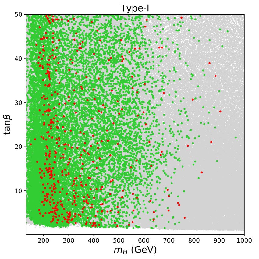
Our parameter scan regions for both Type-I and Type-II are:
π
|α| < , tan β ∈ (0.2, 50), mA ∈ (10, 1500) GeV, mH ± ∈ (10, 1500) GeV ,
2
m12 ∈ (0, 15002 ) GeV2 ,
2
mh = 125.1 GeV, mH ∈ (130, 1500) GeV. (4.21)
We perform a random parameter scan in the above parameter region, with the total number
of samples exceeding 1 billion, for both Type-I and Type-II models.
In figure 8 we show the scan results for the Type-II 2HDM. The grey scatter points
are the regions allowed by B physics, theoretical constraints, heavy Higgs direct searches
and SM Higgs precision measurements at the current LHC Run-II, and constraints from
EW oblique operators. The green points are a subset of the grey ones, which can generate
a SFOEWPT, and the red points are further required to meet the constraints from future
Higgs precision measurements at CEPC. Compared to Case 1 (figure 7), which assumed
the alignment limit and set mH ± = mA , here we could divide the whole allowed region into
4 classes,
• Class A: regions with mH < 350 GeV. Here the region has mH ± ≈ mA > mH , and
the mass splitting
√ is about (300,500) GeV to meet the constraint mH ± > 580 GeV.
Generally λv ≈ 0 to allow for such a large mass splitting and tan β is within
2
the region selected by the theoretical constraints shown in figure 1. This region
can also be divided into two subgroups based on sign(κb ). When sign(κb ) = +,
– 20 –You can also read