No-Reference Image Quality Assessment via Transformers, Relative Ranking, and Self-Consistency

No-Reference Image Quality Assessment via Transformers, Relative Ranking,
 and Self-Consistency

 S. Alireza Golestaneh1 * Saba Dadsetan 2 Kris M. Kitani3
 1
 Bosch Center for AI, Pittsburgh 2 University of Pittsburgh 3 Carnegie Mellon University
arXiv:2108.06858v1 [eess.IV] 16 Aug 2021

 Abstract image is crucial for different computer vision applications
 as well as social and streaming media industries. On a rou-
 The goal of No-Reference Image Quality Assessment tine day, on average several billion photos are uploaded and
 (NR-IQA) is to estimate the perceptual image quality in ac- shared on social media platforms such as Facebook, Insta-
 cordance with subjective evaluations, it is a complex and gram, Google, Flicker, etc; low-quality images can serve
 unsolved problem due to the absence of the pristine refer- as irritants when they convey a negative impression to the
 ence image. In this paper, we propose a novel model to ad- viewing audiences. On the other hand, at one extreme, not
 dress the NR-IQA task by leveraging a hybrid approach that being able to assess the image quality accurately can be life-
 benefits from Convolutional Neural Networks (CNNs) and threatening (e.g., when low-quality images impede the abil-
 self-attention mechanism in Transformers to extract both lo- ity of autonomous vehicles [1, 2] and traffic controllers [3]
 cal and non-local features from the input image. We capture to safely navigate environments).
 local structure information of the image via CNNs, then to Objective image quality assessment (IQA) attempts to
 circumvent the locality bias among the extracted CNNs fea- use computational models to predict the image quality in a
 tures and obtain a non-local representation of the image, manner that is consistent with quality ratings provided by
 we utilize Transformers on the extracted features where we human subjects. Objective quality metrics can be divided
 model them as a sequential input to the Transformer model. into full-reference (reference available or FR), reduced-
 Furthermore, to improve the monotonicity correlation be- reference (RR), and no-reference (reference not available or
 tween the subjective and objective scores, we utilize the rel- NR) methods based on the availability of a reference image
 ative distance information among the images within each [4]. The goal of the no-reference image quality assessment
 batch and enforce the relative ranking among them. Last (NR-IQA) or blind image quality assessment (BIQA) meth-
 but not least, we observe that the performance of NR-IQA ods is to provide a solution when the reference image is not
 models degrades when we apply equivariant transforma- available [5, 6, 7, 8].
 tions (e.g. horizontal flipping) to the inputs. Therefore, NR-IQA mainly divides into two groups, distortion-
 we propose a method that leverages self-consistency as a based and general-purpose methods. A distortion-based ap-
 source of self-supervision to improve the robustness of NR- proach aims to predict the quality score for a specific type
 IQA models. Specifically, we enforce self-consistency be- of distortion (e.g., blocking, blurring). Distortion-based
 tween the outputs of our quality assessment model for each approaches have limited applications in real-world scenar-
 image and its transformation (horizontally flipped) to utilize ios since we cannot always specify distortion types. Thus,
 the rich self-supervisory information and reduce the uncer- a general-purpose approach is designed to evaluate image
 tainty of the model. To demonstrate the effectiveness of our quality without being limited to distortion types. General-
 work, we evaluate it on seven standard IQA datasets (both Purpose methods make use of extracted features that are in-
 synthetic and authentic) and show that our model achieves formative for various types of distortions. Therefore, their
 state-of-the-art results on various datasets.1 performances highly depend on designing elaborate fea-
 tures.
 Traditionally, general-based NR-IQA methods focused
 1. Introduction on quality assessment for synthetically distorted images
 (e.g., Blur, JPEG, Gaussian Noise). However, the
 Being able to predict the perceptual image quality ro-
 main challenges along with existing synthetically distorted
 bustly and accurately without having access to the reference
 datasets are 1) they contain limited content and distortion
 * Work done at Carnegie Mellon University. diversity, and 2) they do not capture complex mixtures of
 1 Code will be released at here. distortions that often occur in real-world images. Recently,

 1

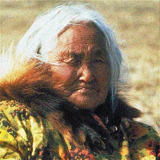
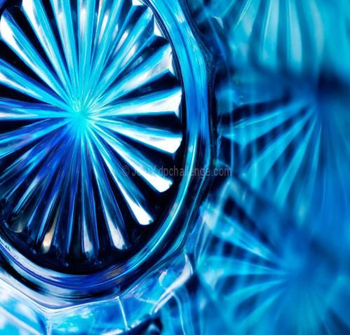
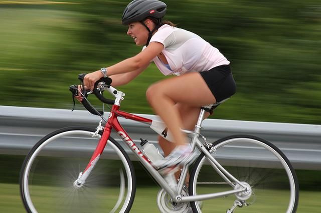
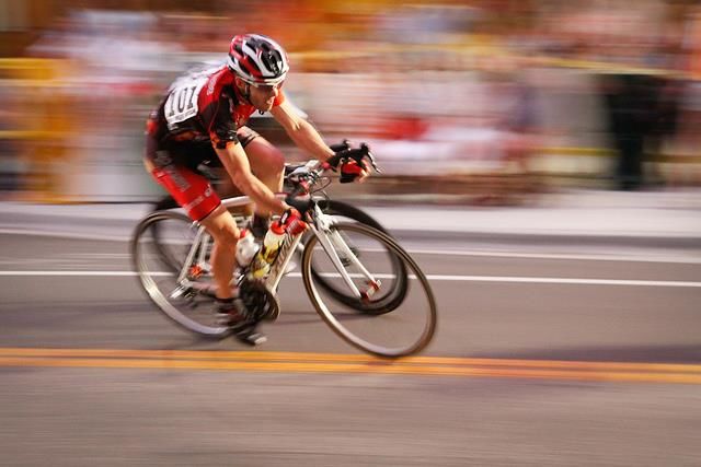
Horizontally
by introducing more in-the-wild datasets such as CLIVE Original
 Flipped
[9], KonIQ-10K [10], and LIVEFB [11] we can have a bet-
ter understanding of complex distortions (e.g., poor lighting MOS = 3.91 MOS = 3.911
 WaDIQaM [38] = 3.42 WaDIQaM [38] = 1.75 (1.67)
conditions, sensor limitations, lens imperfections, amateur HyperIQA [46] = 3.81 HyperIQA [46] = 2.18 (1.63)
 TReS (ours) = 3.79 TReS (ours) = 3.18 (0.61)
manipulations) that often occur in real-world images. In
contrast to synthetic distortions in which degradation pro-
cesses are precisely specified and can be simulated in lab-
oratory environments, authentic distortions are more com- DMOS = 0.489 DMOS = 0.489
 WaDIQaM [38] = 0.224 (0.264)
plicated because there is no reference-image available, and WaDIQaM [38] = 0.488
 HyperIQA [46] = 0.315 HyperIQA [46] = 0.481 (0.166)
 TReS (ours) = 0.472 (0.063)
it is unclear how the human visual system (HVS) distin- TReS (ours) = 0.535

guishes between the picture quality and picture authenticity.
For instance, while distortion can detract from aesthetics, it
can also contribute to it, as when intentionally adding blur MOS = 78.41 MOS = 78.41
 MOS = 2.9
 WaDIQaM
 WaDIQaM [38] = 75.51 WaDIQaM [38] = 62.11 (13.4) HyperIQA
(bokeh) to achieve photographic effects. Moreover, HVS HyperIQA [46] = 72.11 HyperIQA [46] = 84.20 (12.09)
 TReS (ours

perceives image quality differently among various image TReS (ours) = 76.82 TReS (ours) = 72.55 (4.27)

contents and quantifies image quality differently for images
with different contents with the same level and type of dis- Figure 1. Illustration of the sensitivity of NR-IQA models to hor-
tortion [12, 13, 14, 15]. izontal flipping. On the right side of each image, we provide the
 Existing deep learning-based IQA methods mainly rely subjective quality score (MOS/DMOS) and the predicted quality
only on the subjective human scores (MOS/DMOS) and score; the red numbers in the parentheses show the absolute dif-
modeling the quality prediction task mainly as a regression ference between the predictions when the image is flipped.
or classification task. This causes the models not to be able
to leverage the relative ranking between the images explic-
 • We propose a relative ranking loss that explicitly en-
itly. We propose to take into account the relative distance
 forces the relative ranking among the samples. We
information between the images within each batch and en-
 propose to use a triplet loss with an adaptive mar-
force our model to learn the relative ranking between the
 gin based on the human subjective scores to make the
images with the highest and lowest quality scores in addi-
 distance between the image with the highest (lowest)
tion to the quality assessment task.
 quality score closer to the one with the second-highest
 Moreover, as shown in Fig. 1, despite using common (second-lowest) quality score and further away from
augmentation techniques during the training, the perfor- the image with the lowest (highest) score (Sec. 3.4).
mance of IQA methods degrade when we apply a simple
equivariant transformation (e.g., horizontal filliping) to the • Lastly, we propose to use an equivariant transforma-
input image. This contradicts the way that humans perceive tion of the input image as a source of self-supervisory
the quality of images. In other words, subjective percep- to improve the robustness of our proposed model. Dur-
tual quality scores remain the same for specific equivari- ing the training, we use self-consistency between the
ant transformations that can appear very often during real- output for each image and its transformation to uti-
life applications. To alleviate this issue we propose a self- lize the rich self-supervisory information and reduce
consistency approach that enforces our model to have con- the sensitivity of the network (Sec. 3.5).
sistent predictions for an image and its transformed version.
The contributions of this work are summarized as follows: • Extensive experiments on seven benchmark datasets
 (for both authentic and synthetic distortions) confirm
 that our proposed method performs well across differ-
 • We introduce an end-to-end deep learning approach for ent datasets.
 NR-IQA. Our proposed model utilizes local and non-
 local information of an image by leveraging CNNs 2. Related Work
 and self-attention mechanism of Transformers. Partic-
 ularly, in addition to local features that are generated Before the raise of deep learning, early version of
 via CNNs, we take advantage of the sequence model- general-purpose NR-IQA methods mainly divide into natu-
 ing and self-attention mechanism of Transformers to ral scene statistics (NSS) based metrics [16, 17, 6, 5, 18, 19,
 learn a non-local representation of the image from the 8, 20, 21] and learning-based metrics [22, 23, 24, 25, 26,
 multi-scale features that are extracted from different 27]. The underlying assumption for hand-crafted feature-
 layers of CNNs. The non-local features are then fused based approaches is that the natural scene statistics (NSS)
 with the local features to predict the final image quality extracted from natural images are highly regular [28] and
 score (Sec. 3.1, 3.2, and 3.3). different distortions will break such statistical regularities.

 2

Variations of NSS features in different domains such as employs Transformers block to model long-range depen-
spatial [6, 18, 8], gradient [8], discrete cosine transform dencies in language sequence, we utilize a Transformer-
(DCT) [5], and wavelet [17], showed impressive perfor- based network to compute the dependencies among the
mances for synthetically distorted images. Learning-based CNN extracted features from multi-scales and model the
approaches utilize machine learning techniques such as dic- non-local dependency among the extracted features.
tionary learning to map the learned features to the human Transformers were introduced by Vaswani et al. [53] as
subjective scores. Ye et al. [23] used a dictionary learn- a new attention-based building block for machine transla-
ing method to encode the raw image patches to features tion. Attention mechanisms [54] are neural network lay-
and to predict subjective quality scores by support vector ers that aggregate information from the entire input se-
regression (SVR) model. Zhang et al. [26] combined the quence. Due to the success of Transformer-based models
semantic-level features with local features for quality esti- in the NLP field, we start to see different attempts to ex-
mation. Although early versions of hand-crafted and fea- plore the benefits of Transformer for computer vision tasks
ture learning methods perform well on small synthetically [55, 56, 56, 57, 58, 59]. The application of Transformer
distorted datasets, they suffer from not being able to model for NR-IQA is not explored yet. Concurrently with our
real-world distortions. work, [60] used Transformers for NR-IQA, where the fea-
 Deep learning for NR-IQA. By success of deep learn- tures from the last layer of CNNs were sent to Transform-
ing [29, 30] in many computer vision tasks, different ap- ers for the quality prediction task. Different from [60] that
proaches utilize deep learning for NR-IQA [31, 32, 33, 34, use Transformers as an additional feature extraction block
35, 36, 37, 38, 39, 36, 40, 41, 42, 43, 10, 44]. Early version at the end of CNNs, we use it to model the non-local depen-
of deep learning NR-IQA methods [31, 45, 46, 34, 46, 35] dency between the extracted multi-scale features. Notably,
leveraged deep features from CNNs [29, 30] while pre- we leverage the temporal sequence modeling properties of
trained on large classification dataset ImageNet [47]. [48, Transformers to compute a non-local representation of the
49] addressed NR-IQA in a multi-task manner where they image from the multi-scale features (Sec. 3.2).
leverage subjective quality score as well as distortion type Learning to rank for NR-IQA. These approaches [61,
simultaneously during the training. Ma et al. [38] pro- 62, 38, 39] address NR-IQA as a learning-to-rank prob-
posed a multi-task network where two sub-networks train lem, where the relative ranking information is used during
in two stages for distortion identification and quality pre- the training. Zhang et al. [39] leveraged discrete ranking
diction. [50, 51, 52, 36] used some sort of the reference im- information from images of the same content and distor-
ages during their training to predicted the quality score in a tion but at different levels (degree of distortion) for qual-
blind manner. Hallucinated-IQA [36] proposed an NR-IQA ity prediction. [62] used continuous ranking information
method based on generative adversarial models, where they from MOSs and variances between the subjective scores.
first generated a hallucinated reference image to compen- [38, 63] extracted binary ranking information via FR-IQA
sate for the absence of the true reference and then paired the methods during the training. However, due to the use of
information of hallucinated reference with the distorted im- reference images, their method is only applicable to syn-
age to estimate the quality score. Talebi et al. [37] proposed thetic distortions. Existing ranking-based algorithms use
a CNN-based model to predict the perceptual distribution of a fixed margin (which is selected empirically) to minimize
subjective quality scores (instead of the mean value). Zhu et their losses. They also fail to perform well on the authen-
al. [43] proposed a model to leverage meta-learning to learn tic datasets mainly due to the requirement of using referee
the prior knowledge that is shared among different distor- images during the training stage. In our proposed method,
tion types. Su et al. [42] proposed a model that extracts we also leverage the MOS/DMOS information for relative
content features from the deep model in different scales and ranking. However, in contrast to the existing methods, we
pools them to predict image quality. propose to minimize the relative distance among the sam-
 Transformers for NR-IQA. Currently, CNNs are the ples via a triplet loss with an adaptive margin which does
main backbone for features extraction among the state-of- not need the empirical margin selection.
the-art NR-IQA models. Although CNNs capture the lo- Poor generalization in deep neural networks is a well-
cal structure of the image, they are well known for missing known problem and an active area of research. In IQA tasks
to capture non-local information and having strong locality poor generalization is mostly considered as when the model
bias. Furthermore, CNNs demonstrated a bias towards spa- performs well on the dataset that it is trained on but poorly
tial invariance through shared weights across all positions on another dataset with the same type of artifacts. Rea-
which makes them ineffective if a more complex combina- sons such as various contents, domain shift, or scale shift in
tion of features is needed. Since IQA highly depends on the subjective scores mainly cause the poor generalization
both local and non-local features, we propose to use Trans- of IQA models. In our experiments, in addition to cross
formers and CNNs together. Inspired by NLP which widely dataset evaluation, we also notice that the performance of

 3

FC: Fully Connected
 × 1 × 1 × 1
 © : Concatenation
 × 2 × 2 × 2 : Self−Consistency
 × 1 × 4 × 4

 Transformer
 × 3 × 3 × 3

 Normalization
 × ෍ × 4 × 4

 Encoder
 × 1 × 4 × 4

 Dropout
 Pooling
 × 4 × 4 × 4 × 1 × 4 × 4© 
 Pooling + FC
 × 1 × 4 × 4
 Positional
 Encoding FC Quality
 © Scores
 
 Figure 2. Flowchart of our proposed NR-IQA algorithm.

deep-learning based IQA models degrades when we apply features from the last layer in the 4th block of CNN. We
horizontal flipping or rotation to the inputs. Common ap- use the last layers of each block to extract the multi-scale
proaches such as dropout [64], ensembling [65], cross-task features from the input image. Since the extracted features
consistency [66], and augmentation proposed to increase from different layers have different ranges, statistics, and
the generalization in deep models. However, making pre- dimensions, we first send them to normalization, pooling,
dictions using a whole ensemble of models is cumbersome and dropout layers. For normalization and pooling we use
 Fi
and too computationally expensive due to large models’ Euclidean norm which is defined by Fi = max(kF i k2 ,)
 fol-
sizes. Data augmentation has been successful in increas- lowed by a l2 pooling layer [69, 70] which has been used to
ing the generalization of CNNs. However, as shown in Fig. demonstrate the behavior of complex cells in primary visual
1, a model can still suffer from poor generalization for a cortex [71, 72]. The l2 pooling layer defines by:
simple transformation. [67, 68] show that although using p
different augmentation methods improve the generalization P (x) = g ∗ (x x), (1)
of CNNs, they are still sensitive to equivariant perturbations
 where denotes point-wise product, and the blurring ker-
in data.
 nel g(.) is implemented via a Hamming window that ap-
 As shown in Fig. 1, NR-IQA models that used image
 proximately applies the Nyquist criterion [70]. Let F̄i ∈
flipping as an augmentation during training still fail to have
 Rb×ci ×m4 ×n4 denote the output feature after sending Fi to
a robust quality prediction for an image and its flipped ver-
 the normalization, pooling, and dropout layers. Next, we
sion. This kind of high variance in the quality prediction
can affect the robustness of computer vision applications P F̄i , i ∈ {1, 2, 3, 4} and denote it the output by
 concatenate
 F̃ ∈ Rb× i ci ×m4 ×n4 .
directly. In this work, we improve the consistency of our
model via the simple observation that the results of the NR- 3.2. Attention-Based Feature Computation
IQA model should not change under transformations such
as horizontal flipping. CNNs exploit the structure of images via local interac-
 tions through convolution with small kernel sizes. Different
3. Proposed Method layers of a network can have different semantic informa-
 tion that is captured through the local interactions, and as
 In this section, we detail our proposed model, which is we move from lower layers to the higher layers, the com-
an NR-IQA method based on Transformers, Relative rank- puted features carry more semantic about the content of the
ing, and Self consistency, namely TReS. Fig. 2 shows an image [73]. IQA depends on both low- and high-level fea-
overview of our proposed method. tures. A model that does not take into account both low- and
 high-level features can mistake a plain sky as a low-quality
3.1. Feature Extraction
 image [15]. Moreover, due to the architecture of CNNs they
 Given an input image I ∈ R3×m×n , where m and n de- mainly capture the local spatial structure of the image and
note width and height, our goal is to estimate its perceptual are unable to model the relation among the non-local fea-
quality score (q). Let fφ represent a CNN with learnable tures.
parameters φ, and Fi ∈ Rb×ci ×mi ×ni denotes the features Transformers have shown impressive results in modeling
from the ith block of CNN, where i ∈ {1, 2, 3, 4} b de- the dependencies among the sequential data. Therefore, we
notes the batch size, and ci , mi , and ni denote the chan- use the encoder part of the Transformer, which is composed
nel size, width, and height of the ith feature, respectively. of a multi-head self-attention layer and a feed-forward neu-
Let F4 ∈ Rb×c4 ×m4 ×n4 represent the high-level semantic ral network [74, 53, 59] to perform attention operations

 4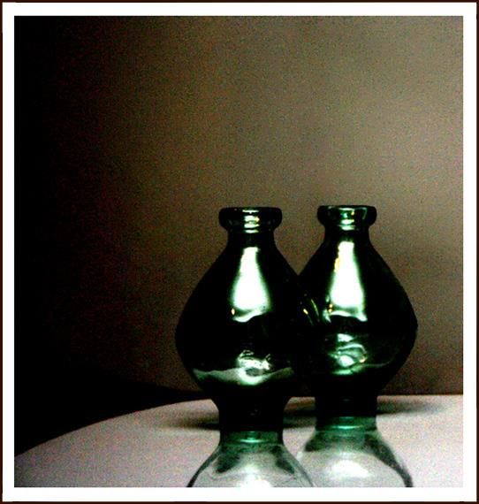

where W1 is the linear projection matrix and has di-
 × mension of d × d, headi = Attention(Qi , Ki , Vi ), and
 T
 Add & Norm Attention(Q, K, V ) = sof tmax( QK √ ) V . For the
Transformer Encoder Layer

 d0
 first Transformer encoder layer, the query, key, and value
 FFN
 matrices (Q, K, and V ) are all the same. Following the
 Add & Norm
 ⨂ Softmax encoder architecture design in [53], to strengthen the flow

 Self-Attention
 of information and improve the performance, a residual
 Multi-Head ⨀ connection followed by a layer normalization is added in
 Self-Attention each sub-layer in the encoder. Next, a feed-forward net-
 V K Q Linear Linear Linear work (FNN) is applied after the self-attention layers [53].
 FNN is consist of two linear transformation layers and a
 ReLU activation function within them, which can be de-
 + noted as F F N (X) = W3 σ(W2 X + b02 ) + b03 , where W2
 Image Positional
 and W3 are the two parameter matrices, and b02 and b03 are
 Features Encoding the biases.Pσ represents the ReLU activation function. Let
 4

Figure 3. Illustration of multi-head multi-layer self-attention
 F̂ ∈ Rb× i ci ×m4 ×n4 represent the output features from
module of the Transformer Encoder layer. N is a hyperparame- the final Transformer encoder layer.
ter that denotes the number of encoder layers In the Transformer 3.3. Feature Fusion and Quality Prediction
which stack together.
 To benefit from the extracted features from both local
 (convolution) and non-local (self-attention) operators we
over the multi-scale extracted features from different lay- use fully connected (FC) layers as fusion layers to map the
ers and model the dependencies among them. We follow aforementioned features and predict the perceptual quality
the encoder architecture of [59] (see Fig. 3). We model of the image (see Fig. 2). For each batch of images, B, we
the features from different layers of CNN as a sequence minimize the regression loss to train our network.
of information (F̃ ) and send them to the Transformer en-
 N
coder. Since the self-attention mechanism is a non-local 1 X
 LQuality,B = kqi − si k , (3)
operation, we use it to compute a non-local representation N i
of the image. In other words, we use Transformers to com-
pute information for each element of extracted features with where qi is the predicted quality score for ith image and si
respect to the others (not only the local neighbor features). is its corresponding ground truth (subjective quality score).
Transformer architecture contains no built-in inductive prior
to the locality of interactions and, is free to learn complex 3.4. Relative Ranking
relationships across the features. We also add positional Although the regression loss (Eq. 3) is effective for the
encoding (in a similar way as [75, 76]) to the input of the quality prediction task, it does not explicitly take into ac-
attention layers to deal with the permutation-invariant prop- count ranking and correlation among images. Here, our
erty of Transformers. The positional encoding will also let goal is to consider the relative ranking relation between the
our model be aware of the position of the features that con- samples within each batch. It is computationally expen-
tribute the most to the IQA task. sive to consider all the samples’ relative ranking informa-
 In detail, given an input (F̃ ) and the number of heads tion; therefore, we only enforce it for the extreme cases.
(h), the input is first transformed into three different groups 0
 Among images within the batch B, let qmax , qmax , qmin ,
of vectors, the query group, the key group and the value 0
 and qmin denote the predicted quality for images with
group. Given a multi-head attention module with h heads highest, second highest, lowest, and second lowest subjec-
and dimension of d, each of the aforementioned groups tive quality scores, respectively, i.e., sqmax > sqmax 0 >
 0
will have dimension of d = hd . Then, features derived sqmin
 0 > sqmin , where sqmax denotes the subjective quality
from different inputs are packed together into three different score corresponding to the image with the predicted qual-
groups of matrices Q0 , K 0 , and V 0 , where Q0 = {Qi }hi=1 = ity score qmax , and a similar notation rule applies to the
Concat(Q1 , ..., Qh ) and the same definition applies to K 0 rest. Our goal is to have d(qmax , qmax 0
 ) + margin1 ≤
and V 0 . Next, the process of multi-head attention is com- d(qmax , qmin ), here we define, d(x, y) as the absolute
puted as follows: value between x and y, d(x, y) = |x − y|. We utilize
 triplet loss to address the above inequality, where we mini-
M ultiHead(Q0 , K 0 , V 0 ) = Concat(head1 , ..., headh )W1 , mize max{0, d(qmax , qmax 0
 ) − d(qmax , qmin ) + margin1 }.
 0
 (2) In a similar way, we also want to have d(qmin , qmin )+

 5

margin2 ≤ d(qmax , qmin ). The margin values can be where τ (B) denote when the equivariant transformation ap-
selected empirically based on each dataset, but that is cum- plies on batch B.
bersome since each dataset have different distributions and
ranges for the quality scores. For a perfect prediction 3.6. Losses
where the estimated quality scores are the same as subjec- Our model trains in an end-to-end manner and minimizes
tive scores we will have the aforementioned losses together simultaneously. The to-
 tal loss for our model is defined as:
 margin1 + sqmax − sqmax
 0 ≤ sqmax − sqmin
 → margin1 + (sqmax − sqmax
 0 ) ≤ (sqmax − sqmin ) (4) Ltotal = LQuality + λ2 LRelative−Ranking +
 (7)
 → margin1 ≤ sqmax
 0 − sqmin . λ3 LSelf −Consistency ,

Therefore, we can consider sqmax0 − sqmin to be an upper- where λ1 , λ2 , λ3 are balancing coefficients.
bound for margin1 during the training, and set margin1 =
sqmax
 0 − sqmin in Eq. 5. Similarly, we define margin2 = 4. Experiments
sqmax − s0qmin . Finally, our relative ranking loss is defined 4.1. Datasets and Evaluation Metrics
as:
 We evaluate the performance of our proposed model ex-
 tensively on seven publicly available IQA datasets (four
LRelative−Ranking,B = synthetically distorted and three authentically distorted).
 0 0
Ltriplet (qmax , qmax , qmin ) + Ltriplet (qmin , qmin , qmax ) For synthetically distorted datasets, we use LIVE [77],
 0
 = max{0, d(qmax , qmax ) − d(qmax , qmin ) + margin1 } CSIQ [78], TID2013 [79], and KADID-10K [80], where
 0 among them KADID has the most number of distortion
 + max{0, d(qmin , qmin ) − d(qmax , qmin ) + margin2 }.
 typesand distorted images. For authentically distorted
 (5)
 datasets, we use CLIVE [9], KonIQ-10k [10], and LIVE-FB
3.5. Self-Consistency [11], where among them LIVE-FB has the most number of
 unique contents. Table 1 shows the summary of the datasets
 Last but not least, we propose to utilize the model’s un- that are used in our experiments.
certainty for the input image and its equivariant transforma-
tion during the training process. We exploit self-consistency Table 1. Summary of IQA datasets.
via the self-supervisory signal between each image and its Databases
 # of Dist. # of Dist. Distortions
equivariant transformation to increase the robustness of the Images Types Type
model. Let for an input I, fφ,conv (I) and fθ,atten (I) de- LIVE 799 5 synthetic
 CSIQ 866 6 synthetic
note the output logits belonging to outputs of the convo- TID2013 3,000 24 synthetic
lution and Transformer layers, respectively, where fφ,conv KADID 10,125 25 synthetic
and fθ,atten represent the CNN and Transformer with learn- CLIVE 1,162 - authentic
able parameters φ and θ, respectively. In our model, we KonIQ 10,073 - authentic
use the outputs of fφ,conv and fθ,atten to predict the im- LIVEFB 39,810 - authentic
age quality and since the human subjective scores stay the
same for the horizontal filliping version of the input im- For performance evaluation, we employ two commonly
age, we thus expect to have fφ,conv (I) = fφ,conv (τ (I)) and used criteria, namely Spearman’s rank-order correlation co-
fθ,atten (I) = fθ,atten (τ (I)), where τ represents the hori- efficient (SROCC) and Pearson’s linear correlation coeffi-
zontal filliping transformation. In this way, by applying our cient (PLCC). Both SROCC and PLCC range from 0 to 1,
consistency loss, the network learns to reinforce representa- and a higher value indicates a better performance. Follow-
tion learning of itself without additional labels and external ing Video Quality Expert Group (VQEG) [83], for PLCC,
supervision. We minimize the self-consistency loss that is logistic regression is first applied to remove nonlinear rating
defined as follows: caused by human visual observation.

 4.2. Implementation Details
 LSelf −Consistency =
 We implemented our model by PyTorch and conducted
 fφ,conv (I) − fφ,conv (τ (I)) + training and testing on an NVIDIA RTX 2080 GPU. Fol-
 fθ,atten (I) − fθ,atten (τ (I)) + lowing the standard training strategy from existing IQA al-
 gorithms, we randomly select multiple sample patches from
 λ1 LRelative−Ranking,B − LRelative−Ranking,τ (B) , each image and horizontally and vertically augment them
 (6) randomly. Particularly, we select 50 patches randomly with

 6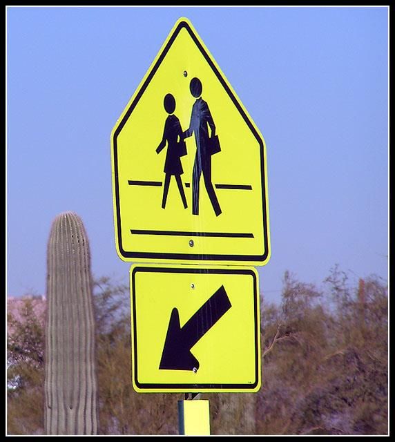

Table 2. Comparison of TReS v.s. state-of-the-art NR-IQA algorithms on synthetically and authentically distorted datasets. Bold entries in
black and blue are the best and second-best performers, respectively. * code were not available publicly.

 LIVE CSIQ TID2013 KADID CLIVE KonIQ LIVEFB Weighted Average
 PLCC SROCC PLCC SROCC PLCC SROCC PLCC SROCC PLCC SROCC PLCC SROCC PLCC SROCC PLCC SROCC
 HFD*[81] 0.971 0.951 0.890 0.842 0.681 0.764 - - - - - - - - - -
 PQR*[35] 0.971 0.965 0.901 0.873 0.864 0.849 - - 0.836 0.808 - - - - - -
 DIIVINE[5] 0.908 0.892 0.776 0.804 0.567 0.643 0.435 0.413 0.591 0.588 0.558 0.546 0.187 0.092 0.323 0.264
 BRISQUE[6] 0.944 0.929 0.748 0.812 0.571 0.626 0.567 0.528 0.629 0.629 0.685 0.681 0.341 0.303 0.457 0.430
 ILNIQE[8] 0.906 0.902 0.865 0.822 0.648 0.521 0.558 0.534 0.508 0.508 0.537 0.523 0.332 0.294 0.430 0.394
 BIECON[82] 0.961 0.958 0.823 0.815 0.762 0.717 0.648 0.623 0.613 0.613 0.654 0.651 0.428 0.407 0.527 0.507
 MEON[38] 0.955 0.951 0.864 0.852 0.824 0.808 0.691 0.604 0.710 0.697 0.628 0.611 0.394 0.365 0.514 0.479
 WaDIQaM[34] 0.955 0.960 0.844 0.852 0.855 0.835 0.752 0.739 0.671 0.682 0.807 0.804 0.467 0.455 0.595 0.584
 DBCNN[39] 0.971 0.968 0.959 0.946 0.865 0.816 0.856 0.851 0.869 0.869 0.884 0.875 0.551 0.545 0.679 0.671
 TIQA[60] 0.965 0.949 0.838 0.825 0.858 0.846 0.855 0.850 0.861 0.845 0.903 0.892 0.581 0.541 0.698 0.670
 MetaIQA[43] 0.959 0.960 0.908 0.899 0.868 0.856 0.775 0.762 0.802 0.835 0.856 0.887 0.507 0.540 0.634 0.656
 P2P-BM[11] 0.958 0.959 0.902 0.899 0.856 0.862 0.849 0.840 0.842 0.844 0.885 0.872 0.598 0.526 0.705 0.658
 HyperIQA[42] 0.966 0.962 0.942 0.923 0.858 0.840 0.845 0.852 0.882 0.859 0.917 0.906 0.602 0.544 0.715 0.676
 TReS (proposed) 0.968 0.969 0.942 0.922 0.883 0.863 0.858 0.859 0.877 0.846 0.928 0.915 0.625 0.554 0.732 0.685

the size of 224×224 pixels from each training image. Train- using the dataset sizes as weights for the performances, and
ing patches inherited quality scores from the source image, we observe that our proposed method outperforms existing
and we minimize Ltotal loss over the training set. We used methods on both PLCC and SROCC.
Adam [84] optimizer with weight decay 5 × 10−4 to train To evaluate the generalizability of our model, in Table
our model for at most 5 epochs, with mini-batch size of 53. 3, we conduct cross dataset evaluations and compare our
The learning rate is first set to 2 × 10−5 and reduced by 10 model to the competing approaches. Training is performed
after every epoch. During the testing stage, 50 patches with on one specific dataset, and testing is performed on a differ-
224 × 224 pixels from the test image are randomly sam- ent dataset without any finetuning or parameter adaptation.
pled, and their corresponding prediction scores are average For synthetic image datasets (LIVE, CSIQ, TID2013), we
pooled to get the final quality score. We use ResNet50 [30] select four distortion types (i.e., JPEG, JPEG2K, WN, and
for our CNN backbone unless mentioned otherwise, while Blur) which all the datasets have in common. As shown in
it is initialized with Imagenet weights. We use N = 2 for Table 3, our proposed method outperforms other algorithms
number of encoder layers in the Transformer, d = 64, and on four datasets among six, which indicate the strong gen-
set the number of heads h = 16. The hyper parameters eralization power of our approach.
λ1 , λ2 , λ3 are empirically set to 0.5, 0.05, 1, respectively.
 Following the common practice in NR-IQA, all experi- Table 3. SROCC evaluations on cross datasets, where bold entries
ments use the same setting, where we first select 10 random indicate the best performers.
 Train on LIVEFB CLIVE KonIQ LIVE
seeds, and then use them to split the datasets randomly to Test on KonIQ CLIVE KonIQ CLIVE CSIQ TID2013
train/test (80%/20%), so we have 10 different splits. Test- WaDIQaM[34] 0.708 0.699 0.711 0.682 0.704 0.462
 DBCNN[39] 0.716 0.724 0.754 0.755 0.758 0.524
ing data is not being used during the training. In the case of P2P-BM[11] 0.755 0.738 0.740 0.770 0.712 0.488
synthetically distorted datasets, the split is implemented ac- HyperIQA[42] 0.758 0.735 0.772 0.785 0.744 0.551
 TReS (Proposed) 0.713 0.740 0.733 0.786 0.761 0.562
cording to reference images to avoid content overlapping.
For all of the reported results we run the experiment 10
times with different random initialization and report the me- We evaluate the latent features learned by our model in
dian SROCC and PLCC values. Fig. 4, where we use the latent features from the last layer
 of the network for query images and collect the top three
4.3. Performance Evaluation nearest neighbor results for the corresponding query. As
 shown in Fig. 4, although we do not explicitly model the
 Table 2 shows the overall performance comparison in content or distortion types in our model, the nearest neigh-
terms of PLCC and SROCC on seven standard image qual- bor samples have similar content or artifacts in terms of
ity datasets, which cover both synthetically and authenti- perceptual quality and have close subjective scores to each
cally distorted images. Furthermore, our model outper- other, which represent the effectiveness of our model in
forms the existing methods by a significant margin on both terms of feature representation. Specifically, in the first row,
LIVEFB and KADID datasets that are currently the largest our model selects images with the same motion blur arti-
datasets for in-the-wild images and synthetically distorted facts as the nearest neighbor samples. In the second row,
images, respectively. Our model also achieves competitive our model selects images with low lighting condition which
results on the smaller datasets. In the last column, we pro- follow similar quality conditions as the query image. The
vide the weighted average performance across all datasets, third row demonstrates the query image that underwent se-

 7

vere JPEG2000 artifacts, and the selected nearest neighbors Table 4. Ablation experiments on the effects of different compo-
 nents for our proposed model.
show that our model has learned the distortion types implic- Psitional Relative Self KADID KonIQ
 Resnet50 Transformer
itly and selects images with the same artifacts as the nearest X
 Encoding Ranking Consistency PLCC SROCC
 0.809 0.802
 PLCC SROCC
 0.873 0.851
neighbors samples. X X X 0.822 0.820 0.896 0.884
 X X 0.833 0.820 0.886 0.872
 X X X 0.840 0.832 0.902 0.0.895
 Query Nearest Neighbor Images X X X X 0.851 0.850 0.918 0.911
 X X X X X 0.858 0.859 0.928 0.915

 Table 5. Ablation experiments on the performance of our proposed
 model via different backbones.
 Dataset Backbone PLCC SROCC Dataset Backbone PLCC SROCC
 Resnet-50 0.877 0.846 Resnet-50 0.942 0.922
 CLIVE Resnet-34 0.855 0.830 CSIQ Resnet-34 0.924 0.920
 MOS = 65.546 MOS = 65.680 MOS = 65.847 MOS = 63.296 Resnet-18 0.859 0.822 Resnet-18 0.911 0.914
 Resnet-50 0.928 0.915 Resnet-50 0.883 0.863
 KonIQ Resnet-34 0.922 0.909 TID2013 Resnet-34 0.847 0.813
 Resnet-18 0.909 0.898 Resnet-18 0.843 0.810
 Resnet-50 0.625 0.560 Resnet-50 0.858 0.859
 LIVEFB Resnet-34 0.619 0.554 KADID Resnet-34 0.851 0.855
 Resnet-18 0.611 0.550 Resnet-18 0.840 0.848

 MOS = 58.1957 MOS =59.3054 MOS = 58.2588 MOS = 59.98918

 4.4. Ablation Study
 In Table 4, we provide ablation experiments to illustrate
 the effect of each component of our proposed method by
 comparing the results on KADID and KonIQ datasets. Fur-
 DMOS = 0.956 DMOS = 0.967 DMOS = 0.977 DMOS = 0. 956 thermore, in Table 5, we evaluate the performance sensi-
Figure 4. Nearest neighbor retrieval results. In each row, the left- tivity of our model for smaller backbones. For a fair com-
most image is a query image, and the rest are the top 3 nearest parison to existing algorithms, we chose Resnet50 for all of
neighbors, using the latent features learned by our proposed mod- the experiments in this paper. However, as shown in Table
els. The nearest neighbor retrieval process is done on the test por- 5, for smaller backbones, our model still achieves compa-
tion of the datasets. Images in the first and second rows are taken rable results. As shown in Table 5, for large datasets (e.g.,
from the LIVEFB dataset, and those on the third row are taken LIVEFB or KonIQ), the performance of our model does not
from the CSIQ dataset. drop significantly and is still competitive when we use a
 smaller backbone, which demonstrates the learning capac-
 ity of our proposed model.

 4.5. Failure Cases and Discussion
 In Fig. 6, we show examples where our method fails
 to predict the image quality in agreement with the human
 subjective scores. All images in Fig. 6 have close ground
 truth scores, and our model predicted different scores for
 each image. From the modeling aspect, we think one rea-
 son for such a failure is that IQA models have to address the
 IQA task as either a regression and/or classification prob-
 lem (simply because the existing datasets provide only the
 quality score(s) for each image). Recently, LIVEFB [11]
 Poor High provides patch-wise quality scores for local patches of each
Quality Quality image and shows that incorporating patch scores leads to
Figure 5. Spatial quality maps generated using the our proposed better performance. As a future direction, we think what
model. Left: Original Images. Right: Quality maps blended with is missing from the existing IQA datasets is a description
the originals using viridis color. of the reasoning process from the subjects to explain the
 reason behind their selected quality score; this can help the
 Moreover, in Fig. 5, we show the spatial quality map future models be able to model the HVS and reasoning be-
generated from the layer with the highest activation in our hind the assigned quality scores in a better way for a more
model. The bright regions represent the poor quality regions precise perceptual quality assessment. On the other hand,
in the input images. from the subjective scores perspective, the subjects may be

 8

less forgiving of the blur artifact and grayscale images, so Transactions on image processing, vol. 21, no. 12, pp. 4695–
those artifacts have drawn their attentions similarly. How- 4708, 2012. 1, 2, 3, 7
ever, our model differentiates between different perceptual [7] W. Xue, L. Zhang, and X. Mou, “Learning without human
cues (color, sharpness, blurriness), which can explain the scores for blind image quality assessment,” in Proceedings
differences in the scores. of the IEEE Conference on Computer Vision and Pattern
 Recognition, 2013. 1
 [8] L. Zhang, L. Zhang, and A. C. Bovik, “A feature-enriched
 completely blind image quality evaluator,” IEEE Transac-
 tions on Image Processing, vol. 24, no. 8, pp. 2579–2591,
 2015. 1, 2, 3, 7
 [9] D. Ghadiyaram and A. C. Bovik, “Massive online crowd-
 sourced study of subjective and objective picture quality,”
 IEEE Transactions on Image Processing, vol. 25, 2015. 2,
 MOS = 62.407 MOS = 62.381 MOS = 62.378 6
 Prediction = 88.021 Prediction = 83.634 Prediction = 63.467
 [10] V. Hosu, H. Lin, T. Sziranyi, and D. Saupe, “Koniq-10k: An
Figure 6. Failure cases, where the predictions are different from
 ecologically valid database for deep learning of blind image
the subjective scores (MOS).
 quality assessment,” IEEE Transactions on Image Process-
 ing, vol. 29, 2020. 2, 3, 6
 [11] Z. Ying, H. Niu, P. Gupta, D. Mahajan, D. Ghadiyaram, and
5. Conclusion A. Bovik, “From patches to pictures (paq-2-piq): Mapping
 In this work, we present an NR-IQA algorithm that the perceptual space of picture quality,” in Proceedings of the
 IEEE Conference on Computer Vision and Pattern Recogni-
works based on a hybrid combination of CNNs and Trans-
 tion, IEEE, 2020. 2, 6, 7, 8
formers features to utilize both local and non-local feature
representation of the input image. We further propose a rel- [12] C.-H. Chou and Y.-C. Li, “A perceptually tuned subband im-
ative ranking loss that takes into account the relative ranking age coder based on the measure of just-noticeable-distortion
 profile,” IEEE Transactions on circuits and systems for video
information among the images. Finally, we exploit an ad-
 technology, vol. 5, 1995. 2
ditional self-consistency loss to improve the robustness of
our proposed method. Our experiments show that our pro- [13] Z. Wang and A. C. Bovik, “Mean squared error: Love it or
 leave it? a new look at signal fidelity measures,” IEEE signal
posed method performs well on several IQA datasets cover-
 processing magazine, vol. 26, no. 1, 2009. 2
ing synthetically and authentically distorted images.
 [14] M. M. Alam, K. P. Vilankar, D. J. Field, and D. M. Chandler,
References “Local masking in natural images: A database and analysis,”
 Journal of vision, vol. 14, 2014. 2
 [1] Y. Lou, Y. Bai, J. Liu, S. Wang, and L. Duan, “Veri-wild: A [15] D. Li, T. Jiang, W. Lin, and M. Jiang, “Which has better
 large dataset and a new method for vehicle re-identification visual quality: The clear blue sky or a blurry animal?,” IEEE
 in the wild,” in Proceedings of the IEEE Conference on Com- Transactions on Multimedia, vol. 21, no. 5, 2018. 2, 4
 puter Vision and Pattern Recognition, 2019. 1
 [16] A. K. Moorthy and A. C. Bovik, “A two-step framework for
 [2] T.-Y. Chiu, Y. Zhao, and D. Gurari, “Assessing image qual- constructing blind image quality indices,” IEEE Signal pro-
 ity issues for real-world problems,” in Proceedings of the cessing letters, vol. 17, no. 5, 2010. 2
 IEEE Conference on Computer Vision and Pattern Recog-
 [17] A. K. Moorthy and A. C. Bovik, “Blind image quality as-
 nition, 2020. 1
 sessment: From natural scene statistics to perceptual qual-
 [3] Z. Zhu, D. Liang, S. Zhang, X. Huang, B. Li, and S. Hu, ity,” IEEE transactions on Image Processing, vol. 20, no. 12,
 “Traffic-sign detection and classification in the wild,” in Pro- pp. 3350–3364, 2011. 2, 3
 ceedings of the IEEE conference on computer vision and pat-
 [18] A. Mittal, R. Soundararajan, and A. C. Bovik, “Making a
 tern recognition, 2016. 1
 “completely blind” image quality analyzer,” IEEE Signal
 [4] Z. Wang and A. C. Bovik, “Modern image quality assess- processing letters, vol. 20, no. 3, pp. 209–212, 2012. 2, 3
 ment,” Synthesis Lectures on Image, Video, and Multimedia
 [19] X. Gao, F. Gao, D. Tao, and X. Li, “Universal blind image
 Processing, vol. 2, 2006. 1
 quality assessment metrics via natural scene statistics and
 [5] M. A. Saad, A. C. Bovik, and C. Charrier, “Blind image qual- multiple kernel learning,” IEEE Transactions on neural net-
 ity assessment: A natural scene statistics approach in the dct works and learning systems, vol. 24, no. 12, 2013. 2
 domain,” IEEE transactions on Image Processing, vol. 21, [20] J. Xu, P. Ye, Q. Li, H. Du, Y. Liu, and D. Doermann, “Blind
 no. 8, 2012. 1, 2, 3, 7 image quality assessment based on high order statistics ag-
 [6] A. Mittal, A. K. Moorthy, and A. C. Bovik, “No-reference gregation,” IEEE Transactions on Image Processing, vol. 25,
 image quality assessment in the spatial domain,” IEEE no. 9, pp. 4444–4457, 2016. 2

 9

[21] D. Ghadiyaram and A. C. Bovik, “Perceptual quality predic- [36] K.-Y. Lin and G. Wang, “Hallucinated-iqa: No-reference im-
 tion on authentically distorted images using a bag of features age quality assessment via adversarial learning,” in Proceed-
 approach,” Journal of vision, vol. 17, no. 1, 2017. 2 ings of the IEEE Conference on Computer Vision and Pattern
[22] P. Ye and D. Doermann, “No-reference image quality assess- Recognition, pp. 732–741, 2018. 3
 ment using visual codebooks,” IEEE Transactions on Image [37] H. Talebi and P. Milanfar, “Nima: Neural image assessment,”
 Processing, vol. 21, no. 7, 2012. 2 IEEE Transactions on Image Processing, vol. 27, no. 8,
[23] P. Ye, J. Kumar, L. Kang, and D. Doermann, “Unsupervised pp. 3998–4011, 2018. 3
 feature learning framework for no-reference image qual- [38] K. Ma, W. Liu, K. Zhang, Z. Duanmu, Z. Wang, and
 ity assessment,” in Proceedings of the IEEE Conference on W. Zuo, “End-to-end blind image quality assessment using
 Computer Vision and Pattern Recognition, IEEE, 2012. 2, 3 deep neural networks,” IEEE Transactions on Image Pro-
[24] L. Zhang, Z. Gu, X. Liu, H. Li, and J. Lu, “Training quality- cessing, vol. 27, no. 3, pp. 1202–1213, 2017. 3, 7
 aware filters for no-reference image quality assessment,” [39] W. Zhang, K. Ma, J. Yan, D. Deng, and Z. Wang, “Blind
 IEEE MultiMedia, vol. 21, 2014. 2 image quality assessment using a deep bilinear convolutional
[25] P. Ye, J. Kumar, and D. Doermann, “Beyond human opinion neural network,” IEEE Transactions on Circuits and Systems
 scores: Blind image quality assessment based on synthetic for Video Technology, vol. 30, 2018. 3, 7
 scores,” in Proceedings of the IEEE Conference on Computer [40] S. Bianco, L. Celona, P. Napoletano, and R. Schettini, “On
 Vision and Pattern Recognition, pp. 4241–4248, 2014. 2 the use of deep learning for blind image quality assessment,”
[26] P. Zhang, W. Zhou, L. Wu, and H. Li, “Som: Semantic ob- Signal, Image and Video Processing, vol. 12, no. 2, 2018. 3
 viousness metric for image quality assessment,” in Proceed- [41] B. Yan, B. Bare, and W. Tan, “Naturalness-aware deep no-
 ings of the IEEE Conference on Computer Vision and Pattern reference image quality assessment,” IEEE Transactions on
 Recognition, pp. 2394–2402, 2015. 2, 3 Multimedia, vol. 21, no. 10, pp. 2603–2615, 2019. 3
[27] K. Ma, W. Liu, T. Liu, Z. Wang, and D. Tao, “dipiq: [42] S. Su, Q. Yan, Y. Zhu, C. Zhang, X. Ge, J. Sun, and Y. Zhang,
 Blind image quality assessment by learning-to-rank discrim- “Blindly assess image quality in the wild guided by a self-
 inable image pairs,” IEEE Transactions on Image Process- adaptive hyper network,” in Proceedings of the IEEE Confer-
 ing, vol. 26, no. 8, pp. 3951–3964, 2017. 2 ence on Computer Vision and Pattern Recognition, pp. 3667–
[28] E. P. Simoncelli and B. A. Olshausen, “Natural image statis- 3676, 2020. 3, 7
 tics and neural representation,” Annual review of neuro- [43] H. Zhu, L. Li, J. Wu, W. Dong, and G. Shi, “Metaiqa: deep
 science, vol. 24, no. 1, pp. 1193–1216, 2001. 2 meta-learning for no-reference image quality assessment,”
[29] A. Krizhevsky, I. Sutskever, and G. E. Hinton, “Imagenet in Proceedings of the IEEE Conference on Computer Vision
 classification with deep convolutional neural networks,” Ad- and Pattern Recognition, 2020. 3, 7
 vances in neural information processing systems, vol. 25, [44] W. Zhang, K. Zhai, G. Zhai, and X. Yang, “Learning to
 2012. 3 blindly assess image quality in the laboratory and wild,” in
[30] K. He, X. Zhang, S. Ren, and J. Sun, “Deep residual learning 2020 IEEE International Conference on Image Processing,
 for image recognition,” in Proceedings of the IEEE confer- pp. 111–115, IEEE, 2020. 3
 ence on computer vision and pattern recognition, pp. 770– [45] S. Bosse, D. Maniry, T. Wiegand, and W. Samek, “A deep
 778, 2016. 3, 7 neural network for image quality assessment,” in 2016 IEEE
[31] L. Kang, P. Ye, Y. Li, and D. Doermann, “Convolutional neu- International Conference on Image Processing, IEEE, 2016.
 ral networks for no-reference image quality assessment,” in 3
 Proceedings of the IEEE conference on computer vision and [46] J. Kim and S. Lee, “Deep learning of human visual sensi-
 pattern recognition, pp. 1733–1740, 2014. 3 tivity in image quality assessment framework,” in Proceed-
[32] J. Long, E. Shelhamer, and T. Darrell, “Fully convolutional ings of the IEEE conference on computer vision and pattern
 networks for semantic segmentation,” in Proceedings of the recognition, 2017. 3
 IEEE conference on computer vision and pattern recogni- [47] J. Deng, W. Dong, R. Socher, L.-J. Li, K. Li, and L. Fei-
 tion, pp. 3431–3440, 2015. 3 Fei, “Imagenet: A large-scale hierarchical image database,”
[33] J. Redmon, S. Divvala, R. Girshick, and A. Farhadi, “You in 2009 IEEE conference on computer vision and pattern
 only look once: Unified, real-time object detection,” in Pro- recognition, pp. 248–255, Ieee, 2009. 3
 ceedings of the IEEE conference on computer vision and pat- [48] L. Kang, P. Ye, Y. Li, and D. Doermann, “Simultaneous esti-
 tern recognition, 2016. 3 mation of image quality and distortion via multi-task convo-
[34] S. Bosse, D. Maniry, K.-R. Müller, T. Wiegand, and lutional neural networks,” in 2015 IEEE international con-
 W. Samek, “Deep neural networks for no-reference and full- ference on image processing, pp. 2791–2795, IEEE, 2015.
 reference image quality assessment,” IEEE Transactions on 3
 Image Processing, vol. 27, 2017. 3, 7 [49] L. Xu, J. Li, W. Lin, Y. Zhang, L. Ma, Y. Fang, and Y. Yan,
[35] H. Zeng, L. Zhang, and A. C. Bovik, “A probabilistic quality “Multi-task rank learning for image quality assessment,”
 representation approach to deep blind image quality predic- IEEE Transactions on Circuits and Systems for Video Tech-
 tion,” arXiv preprint arXiv:1708.08190, 2017. 3, 7 nology, vol. 27, no. 9, 2016. 3

 10

[50] J. Kim and S. Lee, “Fully deep blind image quality predic- [65] Z.-H. Zhou, Ensemble methods: foundations and algo-
 tor,” IEEE Journal of selected topics in signal processing, rithms. CRC press, 2012. 4
 vol. 11, 2016. 3 [66] A. R. Zamir, A. Sax, N. Cheerla, R. Suri, Z. Cao, J. Malik,
[51] J. Kim, A.-D. Nguyen, and S. Lee, “Deep cnn-based blind and L. J. Guibas, “Robust learning through cross-task consis-
 image quality predictor,” IEEE transactions on neural net- tency,” in Proceedings of the IEEE Conference on Computer
 works and learning systems, vol. 30, no. 1, pp. 11–24, 2018. Vision and Pattern Recognition, 2020. 4
 3 [67] D. E. Worrall, S. J. Garbin, D. Turmukhambetov, and G. J.
[52] D. Pan, P. Shi, M. Hou, Z. Ying, S. Fu, and Y. Zhang, “Blind Brostow, “Harmonic networks: Deep translation and rota-
 predicting similar quality map for image quality assessment,” tion equivariance,” in Proceedings of the IEEE Conference
 in Proceedings of the IEEE Conference on Computer Vision on Computer Vision and Pattern Recognition, 2017. 4
 and Pattern Recognition, pp. 6373–6382, 2018. 3
 [68] T. Cohen and M. Welling, “Group equivariant convolutional
[53] A. Vaswani, N. Shazeer, N. Parmar, J. Uszkoreit, L. Jones, networks,” in International conference on machine learning,
 A. N. Gomez, L. Kaiser, and I. Polosukhin, “Attention is all PMLR, 2016. 4
 you need,” arXiv preprint arXiv:1706.03762, 2017. 3, 4, 5
 [69] O. J. Hénaff and E. P. Simoncelli, “Geodesics of learned rep-
[54] D. Bahdanau, K. Cho, and Y. Bengio, “Neural machine resentations,” arXiv preprint arXiv:1511.06394, 2015. 4
 translation by jointly learning to align and translate,” arXiv
 [70] K. Ding, K. Ma, S. Wang, and E. P. Simoncelli, “Image qual-
 preprint arXiv:1409.0473, 2014. 3
 ity assessment: Unifying structure and texture similarity,”
[55] M. Chen and A. Radford, “Rewon child, jeff wu, heewoo jun, arXiv preprint arXiv:2004.07728, 2020. 4
 prafulla dhariwal, david luan, and ilya sutskever. generative
 [71] J. Bruna and S. Mallat, “Invariant scattering convolution net-
 pretraining from pixels,” in Proceedings of the 37th Interna-
 works,” IEEE transactions on pattern analysis and machine
 tional Conference on Machine Learning, vol. 1, 2020. 3
 intelligence, vol. 35, no. 8, 2013. 4
[56] A. Dosovitskiy, L. Beyer, A. Kolesnikov, D. Weissenborn,
 X. Zhai, T. Unterthiner, M. Dehghani, M. Minderer, [72] B. Vintch, J. A. Movshon, and E. P. Simoncelli, “A convolu-
 G. Heigold, S. Gelly, et al., “An image is worth 16x16 words: tional subunit model for neuronal responses in macaque v1,”
 Transformers for image recognition at scale,” arXiv preprint Journal of Neuroscience, vol. 35, no. 44, 2015. 4
 arXiv:2010.11929, 2020. 3 [73] M. D. Zeiler and R. Fergus, “Visualizing and understanding
[57] H. Chen, Y. Wang, T. Guo, C. Xu, Y. Deng, Z. Liu, S. Ma, convolutional networks,” in European conference on com-
 C. Xu, C. Xu, and W. Gao, “Pre-trained image processing puter vision, pp. 818–833, Springer, 2014. 4
 transformer,” arXiv preprint arXiv:2012.00364, 2020. 3 [74] I. Sutskever, O. Vinyals, and Q. V. Le, “Sequence to
[58] K. Han, Y. Wang, H. Chen, X. Chen, J. Guo, Z. Liu, Y. Tang, sequence learning with neural networks,” arXiv preprint
 A. Xiao, C. Xu, Y. Xu, et al., “A survey on visual trans- arXiv:1409.3215, 2014. 4
 former,” arXiv preprint arXiv:2012.12556, 2020. 3 [75] I. Bello, B. Zoph, A. Vaswani, J. Shlens, and Q. V. Le, “At-
[59] N. Carion, F. Massa, G. Synnaeve, N. Usunier, A. Kir- tention augmented convolutional networks,” in Proceedings
 illov, and S. Zagoruyko, “End-to-end object detection with of the IEEE International Conference on Computer Vision,
 transformers,” in European Conference on Computer Vision, 2019. 5
 Springer, 2020. 3, 4, 5 [76] N. Parmar, A. Vaswani, J. Uszkoreit, L. Kaiser, N. Shazeer,
[60] J. You and J. Korhonen, “Transformer for image quality as- A. Ku, and D. Tran, “Image transformer,” in International
 sessment,” arXiv preprint arXiv:2101.01097, 2020. 3, 7 Conference on Machine Learning, PMLR, 2018. 5
[61] F. Gao, D. Tao, X. Gao, and X. Li, “Learning to rank for [77] H. R. Sheikh, M. F. Sabir, and A. C. Bovik, “A statisti-
 blind image quality assessment,” IEEE transactions on neu- cal evaluation of recent full reference image quality assess-
 ral networks and learning systems, vol. 26, no. 10, pp. 2275– ment algorithms,” IEEE Transactions on image processing,
 2290, 2015. 3 vol. 15, 2006. 6
[62] X. Liu, J. van de Weijer, and A. D. Bagdanov, “Rankiqa: [78] E. C. Larson and D. M. Chandler, “Most apparent distortion:
 Learning from rankings for no-reference image quality as- full-reference image quality assessment and the role of strat-
 sessment,” in Proceedings of the IEEE International Confer- egy,” Journal of electronic imaging, vol. 19, no. 1, 2010. 6
 ence on Computer Vision, 2017. 3 [79] N. Ponomarenko, L. Jin, O. Ieremeiev, V. Lukin, K. Egiazar-
[63] K. Ma, X. Liu, Y. Fang, and E. P. Simoncelli, “Blind image ian, J. Astola, B. Vozel, K. Chehdi, M. Carli, F. Battisti, et al.,
 quality assessment by learning from multiple annotators,” in “Image database tid2013: Peculiarities, results and perspec-
 2019 IEEE International Conference on Image Processing, tives,” Signal processing: Image communication, vol. 30,
 pp. 2344–2348, IEEE, 2019. 3 2015. 6
[64] N. Srivastava, G. Hinton, A. Krizhevsky, I. Sutskever, and [80] H. Lin, V. Hosu, and D. Saupe, “Kadid-10k: A large-scale
 R. Salakhutdinov, “Dropout: a simple way to prevent neural artificially distorted iqa database,” in 2019 Eleventh Inter-
 networks from overfitting,” The journal of machine learning national Conference on Quality of Multimedia Experience
 research, vol. 15, 2014. 4 (QoMEX), IEEE, 2019. 6

 11

[81] J. Wu, J. Zeng, Y. Liu, G. Shi, and W. Lin, “Hierarchical fea-
 ture degradation based blind image quality assessment,” in
 Proceedings of the IEEE International Conference on Com-
 puter Vision, pp. 510–517, 2017. 7
[82] J. Kim and S. Lee, “Fully deep blind image quality predic-
 tor,” IEEE Journal on Selected Topics in Signal Processing,
 vol. 11, no. 1, pp. 206–220, 2017. 7
[83] J. Antkowiak, T. Jamal Baina, F. V. Baroncini, N. Chateau,
 F. FranceTelecom, A. C. F. Pessoa, F. Stephanie Colonnese,
 I. L. Contin, J. Caviedes, and F. Philips, “Final report from
 the video quality experts group on the validation of objective
 models of video quality assessment march 2000,” 2000. 6
[84] D. P. Kingma and J. Ba, “Adam: A method for stochastic
 optimization,” arXiv preprint arXiv:1412.6980, 2014. 7

 12