An adaptive method for speeding up the numerical integration of chemical mechanisms in atmospheric chemistry models: application to GEOS-Chem ...
←
→
Page content transcription
If your browser does not render page correctly, please read the page content below
Geosci. Model Dev., 13, 2475–2486, 2020
https://doi.org/10.5194/gmd-13-2475-2020
© Author(s) 2020. This work is distributed under
the Creative Commons Attribution 4.0 License.

An adaptive method for speeding up the numerical integration of
chemical mechanisms in atmospheric chemistry models:
application to GEOS-Chem version 12.0.0
Lu Shen1 , Daniel J. Jacob1 , Mauricio Santillana2,3 , Xuan Wang4 , and Wei Chen5
1 JohnA. Paulson School of Engineering and Applied Sciences, Harvard University, Cambridge, MA, USA
2 Computational Health Informatics Program, Boston Children’s Hospital, Boston, MA, USA
3 Department of Pediatrics, Harvard Medical School, Boston, MA, USA
4 School of Energy and Environment, City University of Hong Kong, Hong Kong SAR, China
5 Department of Physics, Harvard University, Cambridge, MA, USA

Correspondence: Lu Shen (lshen@fas.harvard.edu)

Received: 26 September 2019 – Discussion started: 29 October 2019
Revised: 28 March 2020 – Accepted: 17 April 2020 – Published: 28 May 2020

Abstract. The major computational bottleneck in atmo-            provides the same model output diagnostics (species produc-
spheric chemistry models is the numerical integration of         tion and loss rates, reaction rates) as the full mechanism, and
the stiff coupled system of kinetic equations describing the     can accommodate changes in the chemical mechanism or in
chemical evolution of the system as defined by the model         model resolution without having to reconstruct the chemical
chemical mechanism (typically over 100 coupled species).         regimes.
We present an adaptive method to greatly reduce the com-
putational cost of that numerical integration in global 3-D
models while maintaining high accuracy. Most of the atmo-
                                                                 1   Introduction
sphere does not in fact require solving for the full chemi-
cal complexity of the mechanism, so considerable simplifica-     Accurate representation of atmospheric chemistry is of cen-
tion is possible if one can recognize the dynamic continuum      tral importance for air quality and Earth system models
of chemical complexity required across the atmospheric do-       (National Research Council, 2016), but it is computation-
main. We do this by constructing a limited set of reduced        ally expensive. The complete Master Chemistry Mecha-
chemical mechanisms (chemical regimes) to cover the range        nism (MCM, version 3.3, http://mcm.leeds.ac.uk/MCMv3.
of atmospheric conditions and then pick locally and on the fly   3.1/, last access: November 2019) consists of 5832 species
which mechanism to use for a given grid box and time step        and 16 701 reactions. Atmospheric chemistry models use
on the basis of computed production and loss rates for indi-     greatly simplified mechanisms, which still include hundreds
vidual species. Application to the GEOS-Chem global 3-D          of species coupled through production and loss pathways
model for oxidant–aerosol chemistry in the troposphere and       and with lifetimes ranging from less than 1 s to many years.
stratosphere (full mechanism of 228 species) is presented.       Computing the kinetic temporal evolution of such systems
We show that 20 chemical regimes can largely encompass the       involves solving a stiff system of N coupled non-linear ordi-
range of conditions encountered in the model. Results from a     nary differential equations (ODEs) of the form
2-year GEOS-Chem simulation shows that our method can
reduce the computational cost of chemical integration by         dni
30 %–40 % while maintaining accuracy better than 1 % and             = Pi (n) − Li (n) ,                                    (1)
                                                                  dt
with no error growth. Our method retains the full complex-
ity of the original chemical mechanism where it is needed,       where n = (n1 , . . .nK )T is the vector of species concen-
                                                                 trations, expressed typically as number densities (e.g.,

Published by Copernicus Publications on behalf of the European Geosciences Union.
2476                                                    L. Shen et al.: An adaptive and more efficient chemical mechanism

molecules per cubic centimeter), and K is the number of          and are subject to error growth as simulation time progresses
species in the mechanism. Pi (n) and Li (n) are the produc-      (Keller and Evans, 2019).
tion and loss rates of species i that depend on the concen-         Santillana et al. (2010) combined these ideas in an adap-
trations of other species in the mechanism. Finite-difference    tive algorithm for 3-D models that determines locally at each
solution of the coupled system of ODEs requires an implicit      time step (“on the fly”) which species in the chemical mech-
scheme to avoid limitation of the time step by the short-        anism need to be solved in the coupled implicit system. This
est lifetime in the system (Brasseur and Jacob, 2017). Im-       was done by computing the local production (Pi ) and loss
plicit schemes involve repeated construction and inversion       rates (Li ) for all species at the beginning of the time step.
of the Jacobian matrix (K × K) for the system, and this is       Species with either Pi or Li above a given threshold were
computationally expensive for large K. But the full coupled      labeled “fast” and solved with an implicit scheme, while
chemical mechanism may not be needed everywhere in the           the others were labeled “slow” and solved with an explicit
model domain. For example, highly reactive volatile organic      scheme. The complexity of the chemical system to be solved
compounds (VOCs) have little influence far away from their       was thus adapted to the local environment. Here “fast” and
source regions. Here we show that we can obtain a substan-       “slow” refer to the rates in the chemical system, not the
tial reduction in computational cost in a global 3-D model       species lifetime. For example, short-lived VOCs may be con-
by adaptively adjusting the ensemble of species that actually    sidered slow outside of their source regions because they
need to be solved as a coupled system in a given model grid      have negligible influence on other species. Whether a species
box. We do so with a general algorithm that is readily appli-    is fast or slow depends on the changing local conditions,
cable to any chemical mechanism or numerical solver.             hence the need for an adaptive algorithm, The adaptive ap-
   As the simplest example of an implicit scheme, consider       proach does not prejudge the local environment, unlike in
the first-order method which approximates Eq. (1) as             Jacobson (1995), and instead resolves the dynamic contin-
                                                                 uum of complexity encountered in the atmosphere. Santil-
fi (n(t + 1t)) = ni (t + 1t)−ni (t)−si (n(t + 1t)) 1t, (2)
                                                                 lana et al. (2010) applied their algorithm to the GEOS-Chem
where 1t is the time step and si (n(t+1t)) = Pi (n(t+1t))−       global 3-D Eulerian chemical transport model (Bey et al.,
Li (n(t + 1t)) is the net source evaluated at the end of the     2001). While the computational savings were promising for
time step. This defines a vector function f = (f1 , . . .fK )T   the chemical integration within each grid box, the need to
and an algebraic system f (n(t + 1t)) = 0 that is solved iter-   construct a different system in every single grid box and at
atively by the Newton–Raphson method. The procedure in-          every time step canceled out some of the gains and led to
volves iterative calculation and inversion of the K × K Ja-      only small time savings when compared to the performance
cobian matrix J = ∂s/∂n. Most models use higher-order im-        of the standard full-chemistry model.
plicit algorithms designed for accuracy and speed, such as the      Here we draw from the approach introduced by Santillana
Gear (Gear, 1971; Hindmarsh, 1983) and Rosenbrock (Sandu         et al. (2010) but use a set of pre-defined chemical regimes
et al., 1997; Hairer and Wanner, 1991) solvers, but all re-      to take full advantage of the time savings from the adaptive
quire iteratively calculating the Jacobian matrix and solving    reduction mechanism algorithm. We start with the objective
the linear system using a matrix factorization. As a result,     identification of a limited number of chemical regimes that
the chemical operator that solves for the chemical evolution     encompass the range of atmospheric conditions encountered
of species concentrations from Eq. (1) is the most expen-        in the model. These regimes are defined by the subset of fast
sive component of atmospheric chemistry models (Eastham          species from the full mechanism that need to be considered
et al., 2018), and this computational cost has been a barrier    in the coupled system, and we pre-code the Jacobian matrix
for inclusion of atmospheric chemistry in Earth system mod-      and its inverse for each. The model then picks the appro-
els (National Research Council, 2012).                           priate chemical regime to be solved locally and on the fly.
   There are various ways to speed up the chemical operator,     We show that this approach can achieve large computational
all involving some loss of accuracy or generality (Brasseur      savings without significantly compromising accuracy when
and Jacob, 2017). A general approach is to reduce the di-        implemented in GEOS-Chem. Our method can be adapted to
mension of the coupled system of ODEs that needs to be           any mechanism and model, retains the complexity of the full
solved implicitly. This can be done by simplifying the chem-     mechanism where it is needed, and preserves full diagnos-
ical mechanism to decrease the number of species (Brown-         tic information on chemical evolution (such as reaction rates
Steiner et al., 2018; Sportisse and Djouad, 2000) or by          and production and loss of individual species).
isolating long-lived species for which a fast explicit solu-
tion scheme is acceptable (Young and Boris, 1977). Jacob-
son (1995) used different subsets of their full mechanism        2   Model description
to simulate the urban atmosphere, the troposphere, and the
stratosphere. Machine learning algorithms have been devel-       We use the GEOS-Chem 12.0.0 global 3-D
oped to replace the role of the conventional chemical solver;    model for tropospheric and stratospheric chemistry
but these methods have only been applied to simple scenarios     (https://doi.org/10.5281/zenodo.1343547) as a demon-

Geosci. Model Dev., 13, 2475–2486, 2020                                          https://doi.org/10.5194/gmd-13-2475-2020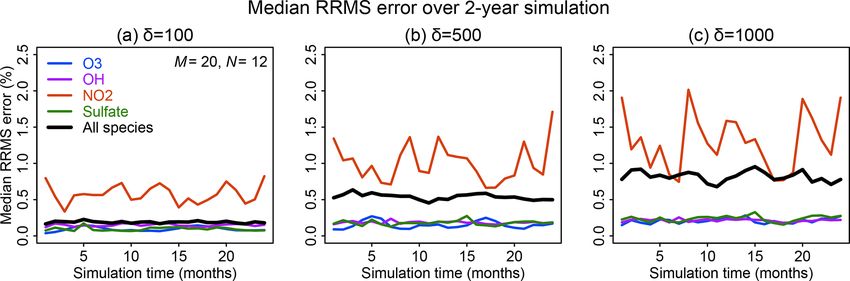
L. Shen et al.: An adaptive and more efficient chemical mechanism                                                              2477

stration for our algorithm. The model is applied here with            δ or Li (n) ≥ δ; slow if Pi (n) < δ and Li (n) < δ. Concen-
a horizontal resolution of 4◦ × 5◦ and 72 pressure levels             trations of the fast species are integrated as a coupled sys-
extending from the surface to 0.01 hPa. It is driven by               tem with the KPP Rosenbrock solver. Concentrations of
MERRA2 assimilated meteorological data from the NASA                  slow species are integrated by explicit analytical solution of
Global Modeling and Assimilation System (GMAO). The                   Eq. (1) assuming first-order loss with effective rate coeffi-
model includes coupled gas-phase and aerosol chemistry as             cient ki = Li /ni :
described by Sherwen et al. (2016) and Travis et al. (2016)
                                                                      dni
for the troposphere and Eastham et al. (2014) for the                       = Pi − ki ni ,                                       (3)
stratosphere. The chemical mechanism has 228 species                   dt
and 724 reactions. Among these species, 143 are volatile                              Pi (t)            Pi (t) −ki (t)1t
                                                                      ni (t + 1t) =          + ni (t) −          e       .       (4)
organic compounds (VOCs), 37 are inorganic reactive                                   ki (t)            ki (t)
halogen species, 24 are organic halogen species, and 24 are           Solving for ni (t + 1t) by Eq. (4) incurs negligible compu-
other inorganic and aerosol species. The chemical reactions           tational cost; therefore, there is considerable advantage in
are integrated using the Rosenbrock solver (Sandu et al.,             classifying species as slow if this can be done without signif-
1997; Hairer and Wanner, 1991) generated from the Kinetic             icant loss in accuracy. We select the threshold δ for species
PreProcessor 2.2.4 (KPP) (Damian et al., 2002) software.              to be classified as fast or slow by numerical testing, as de-
The model uses operator splitting between chemistry and               scribed in Sect. 4, but some basic chemical reasoning is use-
transport with a chemistry time step of 20 min (Philip et             ful. Consider the OH radical, which is a central species in
al., 2016). We use 12 cores with shared memory in the                 atmospheric chemistry mechanisms. OH has a daytime con-
simulations.                                                          centration of the order of 106 molecules cm−3 and a lifetime
   The key processes in the KPP chemical operator are as fol-         of the order of 1 s, implying production and loss rates of
lows. The operator first updates the reaction rate coefficients       the order of 106 molecules cm−3 s−1 . Species with produc-
on the basis of temperature, actinic flux, etc. It then passes        tion and loss rates that are orders of magnitude lower than
these reaction rate coefficients together with initial species        106 molecules cm−3 s−1 are therefore unlikely to influence
concentrations to the Rosenbrock solver, which solves for the         OH or other species in the coupled mechanism, as these are
temporal evolution of concentrations over the external time           all to some extent related to OH at least in the daytime. So
step 1t. In the process, the Rosenbrock solver approximates           we may expect an appropriate threshold δ to be of the order
the solution at multiple internal time steps, so it needs to          of 102 –103 molecules cm−3 s−1 . Santillana et al. (2010) rec-
repeatedly recompute the species production and loss rates,           ommended δ = 100 molecules cm−3 s−1 in their algorithm.
construct the corresponding Jacobian matrix, and solve the               One issue with the solution for the slow species by Eq. (4)
linear system numerically using a matrix factorization. The           is that it does not strictly conserve mass, because the loss
bulk of the cost in the overall chemical operator is in the re-       rate for a given species over the time step does not necessar-
peated computation of production or loss rates and in solving         ily match the production rate of the product species. This is
the linear system using a matrix factorization. Reducing the          usually inconsequential, but we found in early testing that it
number of species in the system to be solved can significantly        resulted in the total mass of reactive halogen species growing
reduce the computational cost.                                        slowly over time in the stratosphere. To avoid this effect, we
                                                                      treat all 37 reactive inorganic halogen species as fast above
                                                                      10 km altitude. This increases the computation cost of chem-
3     The adaptive algorithm for the chemical operator                ical integration by only 4 % relative to letting the algorithm
                                                                      set them as either fast or slow.
Our adaptive algorithm determines locally and on the fly
what degree of complexity is needed in the chemical mech-             3.2   Preselecting the chemical regimes
anism by diagnosing all species in the full chemical mech-
anism as either “fast” or “slow”, and choosing among                  Instead of building a local chemical mechanism subset at ev-
pre-constructed chemical mechanism subsets (“chemical                 ery time step as in Santillana et al. (2010), we greatly im-
regimes”) which is most appropriate for the local conditions.         prove the computational efficiency by preselecting a lim-
Here we present (1) the definition of fast and slow species           ited number (M) of chemical mechanism subsets (chemical
and the different treatments for each and (2) the approach            regimes) for which we pre-define the Jacobian matrix in KPP.
used to pre-construct the chemical regimes.                           We then determine locally which chemical regime to apply
                                                                      on basis of the ensemble of species classified as fast. This
3.1    Definition of fast and slow species                            approach reduces the computational overhead of repeatedly
                                                                      allocating and de-allocating memory in the method of San-
Following Santillana et al. (2010), we separate atmospheric           tillana et al. (2010).
species as fast or slow based on their production and loss                Construction of the chemical regimes can be done objec-
rates in Eq. (1) relative to a threshold δ: fast if either Pi (n) ≥   tively by searching for a minimum in the computational cost

https://doi.org/10.5194/gmd-13-2475-2020                                                Geosci. Model Dev., 13, 2475–2486, 2020
2478 L. Shen et al.: An adaptive and more efficient chemical mechanism
of the chemical operator over the global domain. But some
narrowing of the search is necessary. For the 228-species
mechanism in GEOS-Chem, there are in principle 2228 −1
possible combinations of species that would form mecha-
nism subsets. The vast majority of those combinations make
no chemical sense, but diagnosing this objectively would be
computationally unfeasible. Instead, we start by splitting the
mechanism species into N different blocks based on similar-
ity of chemical behavior. Then we classify a block as fast if
at least one species in the block is fast and slow if all species
in the block are slow. The chemical regime is defined as the
assemblage of fast blocks.
The partitioning of species into blocks can be optimized
by minimizing globally the number of fast species (and hence
the computation cost) for a given threshold δ. We use for this
purpose a training dataset from a GEOS-Chem simulation for
2013, consisting of the global ensemble of tropospheric and
stratospheric grid boxes for the first 10 d of February, May, Figure 1. The diagram for calculating the cost function Z2 .
August, and November sampled every 6 h (160 time steps in
total). To reduce the computational cost, we optimize the par-
titioning of species into blocks for each individual time step, ning the optimization multiple times and using different tem-
resulting in 160 different partitionings, and we then select the perature parameters.
partitioning that yields the lowest cost function when applied Once the blocks have been defined in the above manner,
to all time steps. we define the chemical regimes as different assemblages of
For each grid box j , we diagnose each individual species blocks. This yields 2N −1 possible chemical regimes. Indi-
i as fast or slow following Sect. 3.1. We then diagnose the vidual grid boxes in the model domain may correspond to
blocks as fast or slow with the indicator yi,j = 1 if the block any of these 2N –1 regimes at any given time depending on
is fast (at least one species in the block is fast) or yi,j = 0 which blocks are classified as fast or slow. We need to limit
if the block is slow (all species in the block are slow). The the number of regimes to a much smaller number Mof most
fraction Z1 of all species that needs to be treated as fast over useful regimes in order to keep the compilation of the code
the testing domain is then given by manageable. In fact, as we will see, the bulk of conditions
in the model domain can effectively be represented by just a
few regimes. Grid boxes that do not correspond to any of the
1 XX
Z1 = yi,j , (5) M regimes need to be matched to one of the M regimes by
j i moving some blocks from slow to fast, which will change the
values of the corresponding indicators yi,j from 0 to 1. We
where = 195 408 is the total number of grid boxes in check each of the M regimes and select the one that needs
the troposphere and stratosphere (195 408 grid boxes, cor- the least number of moves from slow to fast, and this se-
responding to the 59 lower levels of the model up to the lection can be pre-defined so it does not add extra compu-
∗ as the indicators adjusted by
tational time. We refer to yi,j
stratopause) multiplied by the total number of species (228 in
our case). We seek the partitioning of species into blocks that these changes. Thus, the fraction Z2 of species that needs to
will minimize Z1 , and we use for that purpose the simulated be treated as fast over the global domain is given by
annealing algorithm (Kirkpatrick et al., 1983). Starting from !
an arbitrary partitioning of the 228 species into N blocks, 1 XX XX
∗
Z2 = yi,j + yi,j , (6)
and at each iteration of the algorithm, we randomly move D i D i
1 2
one species from one block to another. If Z1 decreases, this
transition is accepted; if not, the transition is accepted with a where D1 is the grid boxes that can be represented by the
probability controlled by a parameter named temperature that M chemical regimes and D2 is the grid boxes that are rep-
decreases gradually as the algorithm proceeds. Among the resented by other regimes and must be matched to the M
N blocks, three are allocated to the reactive inorganic halo- regimes. At the beginning of each time step, we pick the
gen species, and N-3 are allocated to the other species. This chemical regime to use for each grid box on the basis of
forced separation of the reactive inorganic halogen species computed production and loss rates for individual species.
is because the corresponding blocks are imposed to be fast A diagram for this process can be found in Fig. 1.
above 10 km altitude (see Sect. 3.1). Throughout this study, We tested a range of values from 5 to 20 for the num-
we present the results with the lowest cost function after run- ber N of blocks. In this testing we used a threshold δ =
Geosci. Model Dev., 13, 2475–2486, 2020 https://doi.org/10.5194/gmd-13-2475-2020L. Shen et al.: An adaptive and more efficient chemical mechanism 2479
Figure 2. Minimum of cost function Z2 (global fraction of chemi-
cal species treated as fast) as a function of the number N of blocks
used to group the species for mechanism reduction. Values were
computed using the GEOS-Chem troposphere + stratosphere sim-
ulation on the first days of February, April, August, and Novem-
ber 2013, over 24 h and sampled every 6 h. Shaded area shows the
standard deviation of the cost function minimum computed for each
Figure 3. Speedup of the chemical computation as a function of the
sample.
number M of chemical mechanism subsets (chemical regimes) used
in the coupled implicit solver of the GEOS-Chem model for adap-
tive simulation of the troposphere and stratosphere. (a) Minimum
of cost function Z2 (global fraction of chemical species treated as
100 molecules cm−3 s−1 to partition fast and slow species, fast) as a function of the number of chemical regimes. (b) Percent-
following Santillana et al. (2010), and a number M = 20 of age of model grid boxes that can be represented by the M chemical
chemical regimes (see next paragraph for choice of M). Fig- regimes without adjustment (see Eq. 5 and related text). Dashed
ure 2 shows the fraction of fast species in the global domain lines show the values for M = 20. For both panels, results are for
(Z2 ) as a function of N. If N is low such that blocks are large, the first 10 d of February, May, August, and November sampled ev-
there is more likelihood that a species in a given block will ery 6 h (shaded area denotes 1 standard deviation of results sampled
be fast, causing all species in the block to be treated as fast. every 6 h).
If N is high, more blocks will need to be moved from slow
to fast in order to match the limited number M of chemical
regimes. For M = 20 we thus find an optimal value N = 12 (e.g., block 6). In addition, there are still noticeable changes
at which only 40 % of the species need to be treated as fast in species groups if we run the simulated annealing algorithm
in the global tropospheric and stratospheric domain. with different initializations and choices of the temperature
Table 1 lists the species of these 12 blocks. Oxidants such parameter, even though the optimized blocks can generally
as OH, O3 , and NO2 are important under all circumstances separate the oxidants, anthropogenic VOCs, and biogenic
so blocks 8 and 9 are fast in most grid boxes. Non-methane VOCs (Table S1 in the Supplement). These two shortcom-
VOC species often have low concentrations outside of the ings may be addressed by introducing regularization terms
continental boundary layer and very low concentrations in in the cost function to enforce known species relationships.
the stratosphere, so the dominant VOC blocks 1–7 are fast in We will implement this in follow-up work.
fewer than 40 % of grid boxes. Anthropogenic VOC species We tested different numbers of chemical regimes (M)
(blocks 4 and 5) are found to be fast in the boundary layer from 3 to 40 for combining the N = 12 blocks and again
and daytime mid-troposphere (Figs. S1–S2 in the Supple- selected the regimes to minimize the global fraction Z2 of
ment). Biogenic VOC species have shorter lifetimes, so they species to be included in the implicit solver. Z2 decreases
are found to be fast only in the lower and middle troposphere from 65 % to 40 % as M increases from 3 to 20 and flat-
over land (Figs. S3–S4). tens at higher values of M (Fig. 3a). This is because 88 %
This algorithm still has shortcomings. There are some un- of the grid boxes can be represented by 20 chemical regimes
expected groupings (such as sulfur species and peroxyacetyl (Fig. 3b). A larger number of blocks (N > 12) would extend
nitrate) and separations (such as HO2 and H2 O2 ). The blocks the improvement to higher values of M, but the size of M
are constructed by minimizing the number of fast species in is also limited by considerations of code manageability and
the optimization, so species tend to be in the same block as compilation speed. We use 20 chemical regimes in what fol-
long as they are fast or slow simultaneously. For example, lows.
isoprene products and CFCs are both slow in the stratosphere Table 2 shows the composition of the 20 chemical regimes
and clean regions, so they may be assigned to the same group as defined by the blocks of Table 1. For 72 % of the grid
https://doi.org/10.5194/gmd-13-2475-2020 Geosci. Model Dev., 13, 2475–2486, 20202480 L. Shen et al.: An adaptive and more efficient chemical mechanism
Table 1. Partitioning of GEOS-Chem chemical species into N = 12 blocks.a
Block Type of Number of Species Percentage of grid
speciesb species boxes where fastc
1 Aromatics 21 CH2I2, LBRO2H, LBRO2N, LTRO2H, LTRO2N, 33.4
SO4H2, IMAE, BENZ, TOLU, TRO2, BRO2, CH2Cl2,
IMAO3, RA3P, RP, PP, IPMN, GLYX, A3O2, PO2,
R4N1
2 Organic nitrates 7 INDIOL, SO4H1, PPN, IONITA, N, RCO3, R4N2 39.3
3 Isoprene, terpenes 30 CH2ICl, LISOPOH, LISOPNO3, MONITA, OCS, 13.9
CHBr3, CHCl3, HCFC22, PRPN, HPALD, HONIT,
RIPB, RIPA, LIMO, MONITS, ISOPNB, CH3CHOO,
MVKN, PRN1, MONITU, CH2OO, PROPNN, ISOP,
OLND, OLNN, HC5OO, ISN1, HC5, RIO2, INO2
4 Alkanes, alkenes, acetone 12 MSA, MAP, ETP, SO4, ATOOH, C2H6, ATO2, ACTA, 41.4
ACET, ETO2, PRPE, ALD2
5 Higher alkanes, methyl ethyl 14 CH3I, RB3P, CH3Cl, ALK4, R4P, C3H8, EOH, B3O2, 36.5
ketone KO2, MGLY, R4O2, HAC, RCHO, MEK
6 Halocarbons, isoprene products 55 CH2IBr, ISN1OA, ISN1OG, LVOCOA, LVOC, PYAC, 10.2
SOAMG, DHDN, CH3CCl3, H1301, H2402, PMNN,
CCl4, CFC11, CFC12, CFC113, CFC114, CFC115,
H1211, IEPOXD, CH2Br2, HCFC123, HCFC141b,
HCFC142b, CH3Br, DHPCARP, IAP, HPC52O2,
MOBA, ISNP, MAOP, MRP, RIPD, ETHLN, ISNO-
HOO, NPMN, MOBAOO, DIBOO, ISNOOB, INPN,
MACRNO2, MVKOO, GAOO, MGLYOO, MGLOO,
MAN2, ISNOOA, ISOPNDO2, MACROO, MACRN,
MAOPO2, LIMO2, ISOPNBO2, ISOPND, NMAO3
7 Secondary organic aerosol 25 LXRO2H, LXRO2N, SOAGX, SOAIE, SOAME, 15.6
DHDC, IEPOXA, IEPOXB, XRO2, XYLE, PIP,
HC187, VRP, DHMOB, MTPA, MTPO, ROH,
IEPOXOO, HCOOH, PIO2, GLYC, VRO2, MRO2,
MACR, MVK
8 Sulfur, peroxyacetyl nitrate 15 CO2, N2O, DMS, HNO4, HNO2, PAN, MP, H, CH4, 95.9
H2O2, MCO3, SO2, CO, O1D, O
9 Oxidants 12 MPN, N2O5, HNO3, CH2O, MO2, O3, NO, HO2, 100.0
NO3, NO2, H2O, OH
10 Iodine reservoirs 13 AERI, ISALA, ISALC, I2O4, I2O3, IBr, INO, HI, ICl, 69.5
ClNO2, BrSALC, BrSALA, I2
11 Bromine and chlorine inorganic 11 ClOO, BrCl, Br2, BrNO3, HOBr, HOCl, ClNO3, Cl, 99.9
species HBr, ClO, HCl
12 Bromine and iodine radicals 13 I2O2, BrNO2, Cl2O2, IONO, OIO, OClO, HOI, 85.0
IONO2, Cl2, I, IO, BrO, Br
a The full GEOS-Chem mechanism has 228 species. The full names of these acronyms can be found at
http://wiki.seas.harvard.edu/geos-chem/index.php/Species_in_GEOS-Chem (last access: November 2019). Results in columns 2–4 are obtained using data from the first 10 d of
February, May, August, and November sampled every 6 h. b Qualitative descriptor of the most important species in the block. c Global percentage of GEOS-Chem model grid
boxes in the troposphere and stratosphere where the block is treated as fast. Values are for 1 August 2013 sampled every 6 h.
Geosci. Model Dev., 13, 2475–2486, 2020 https://doi.org/10.5194/gmd-13-2475-2020L. Shen et al.: An adaptive and more efficient chemical mechanism 2481
boxes in the troposphere and stratosphere, we only need to
solve for fewer than 50 % of the species as fast. Only 3.6 %
of grid boxes need to use the full chemistry mechanism, as
defined by the 20th regime.
Figure 4 shows the distribution of these 20 chemical
regimes globally and for different altitudes and the corre-
sponding percentage of fast species that needs to be included
in the chemical solver. In continental surface air where VOC
emissions are concentrated, we find that over 80 % of species
generally need to be included. This percentage is reduced
to 20 %–60 % over the ocean and < 20 % over Antarctica.
At 5 km altitude, we find a distinct boundary between the
daytime and nighttime hemisphere; the daytime chemistry
is more active, and the percentage of fast species is higher
in the daytime (40 %–60 %) than at night (10 %–30 %). At
15 km altitude the extratropics are in the stratosphere, where
non-methane VOC chemistry is largely absent, but the model
still needs to solve 30 %–40 % species as fast because of
the halogens. Deep convection over tropical continents de-
livers short-lived VOCs and their oxidation products to the
upper troposphere, so that a large number of species needs
to be treated as fast in the convective outflow where and
when it occurs. The importance of deep convective outflow
for global atmospheric chemistry has been pointed out in a
number of studies (Prather and Jacob, 1997; Bechara et al.,
2010; Schroeder et al., 2014) and emphasizes the advantage
of reducing the mechanism adaptively on the fly rather than
with preset geographic boundaries.
Figure 4. Chemical mechanism complexity needed in different re-
gions of the atmosphere. The figure identifies the chemical regime
4 Error analysis from Table 2 needed to simulate a given GEOS-Chem grid box on
1 August 2013 at 00:00 and 12:00 GMT. The percentage of the 228
Here we quantify the errors in our adaptive reduced mecha- species treated as fast (requiring coupled implicit solution) in that
nism method by comparison with a standard GEOS-Chem chemical regime is shown on the color bar and more details are in
simulation for the troposphere and stratosphere (version Tables 1 and 2. Results are shown for different altitudes and using a
threshold δ of 100 molecules cm−3 s−1 .
12.0.0) including full chemistry (228 species). The compar-
ison is conducted for a 1-month simulation to examine the
sensitivity to the rate threshold δ and for a 2-year simula-
tation but at the expense of accuracy. We tested different rate
tion to evaluate the stability of the method. In both cases, we
thresholds ranging from 10 to 5000 molecules cm−3 s−1 in a
use the relative root mean square (RRMS) metric as given by
1-month GEOS-Chem simulation starting on 1 August 2013.
Sandu et al. (1997) to characterize the error:
Figure 5 shows the median RRMS error for all species on
v
u !2 1 September and the increased computational performance
u 1 X
u Qi nreduced
i,j − nfull
i,j for different rate thresholds δ. The best range for δ is be-
RRMSi = t , (7) tween 100 and 1000 molecules cm−3 s−1 , where the median
Qi j =1 nfull
i,j
RRMS error is below 1 % and the improvement in computa-
tional performance is in the 30 %–40 % range.
where nreduced
i,j and nfull
i,j are the concentrations for species i Figure S5 further shows the distribution of RRMS
and grid box j in the reduced and full chemical mechanisms, errors over all species for different rate thresholds δ.
and the sum is over the Qi grid boxes where nfull i,j is greater The 90th percentile RRMS error stays below 5 % if
than a threshold a. Here we use a = 1 × 10⁶ molecules cm−3 δ ≤ 1000 molecules cm−3 s−1 but exceeds 10 % for δ =
as in Eller et al. (2009) and Santillana et al. (2010). 5000 molecules cm−3 s−1 . The 99th percentile RRMS error
A critical parameter to select in the algorithm is the rate is less than 20 % for δ ≤ 1000 molecules cm−3 s−1 but rises
threshold δ separating fast and slow species on the basis of to 80 % for δ = 5000 molecules cm−3 s−1 . The largest errors
their production and loss rates. A high threshold decreases are usually from the tropospheric halogen species (Fig. S6).
the number of fast species and hence speeds up the compu- When near the day–night terminator, the sharp transition of
https://doi.org/10.5194/gmd-13-2475-2020 Geosci. Model Dev., 13, 2475–2486, 20202482 L. Shen et al.: An adaptive and more efficient chemical mechanism
Table 2. Composition and frequency of the 20 chemical regimes in the adaptive algorithma .
Regime no. Block Percentage of Percentage of
fast speciesb grid boxesc
1 2 3 4 5 6 7 8 9 10 11 12
1 0 0 0 0 0 0 0 0 1 0 0 0 5.6 0.1
2 0 0 0 0 0 0 0 0 1 0 1 0 10.3 3.9
3 0 0 0 0 0 0 0 0 1 0 1 1 15.8 0.1
4 0 0 0 0 0 0 0 1 1 0 1 0 18.4 5.4
5 0 1 0 0 0 0 0 1 1 0 1 0 21.4 2.2
6 0 0 0 0 0 0 0 1 1 0 1 1 23.9 0.5
7 0 1 0 0 0 0 0 1 1 0 1 1 26.9 0.2
8 0 1 0 1 0 0 0 1 1 0 1 0 26.9 1.1
9 0 0 0 0 0 0 0 1 1 1 1 1 29.5 46.3
10 0 0 0 1 0 0 0 1 1 0 1 1 29.5 0.5
11 0 0 0 1 0 0 0 1 1 1 1 1 35.0 3.3
12 0 0 0 1 1 0 0 1 1 0 1 1 35.5 0.7
13 0 1 0 1 1 0 0 1 1 0 1 1 38.5 2.4
14 1 1 0 1 1 0 0 1 1 0 1 1 47.4 5.2
15 1 1 0 1 1 0 0 1 1 1 1 1 53.0 12.7
16 1 1 0 1 1 0 1 1 1 0 1 1 58.1 1.7
17 1 1 1 1 1 0 1 1 1 1 1 1 76.5 3.7
18 1 1 1 1 1 1 1 1 1 0 1 0 88.9 2.3
19 1 1 1 1 1 1 1 1 1 0 1 1 94.4 4.4
20 1 1 1 1 1 1 1 1 1 1 1 1 100.0 3.6
a The chemical regimes are defined by the ensemble of fast species that need to be treated as a coupled system with an implicit solution in
the chemical operator. The species are assembled into blocks as listed in Table 1, and here we identify the blocks treated as fast in the
chemical regime (1 ≡ fast, 0 ≡ slow). b Percentage of the 228 species in the GEOS-Chem chemical mechanism treated as fast in the
chemical regime. c Global percentage of GEOS-Chem tropospheric and stratospheric grid boxes for which the chemical regime is
selected. Values are for 1 August 2013 sampled every 6 h.
production and loss rates is not properly captured by the first- 5 Conclusions
order explicit equations, resulting in high relative errors.
Figure 6 shows the time evolution over 2 years of sim-
ulation of the median RRMS error for all species and also We have presented an adaptive method to speed up the tem-
for the selected species OH, ozone, sulfate, and NO2 . The poral integration of chemical mechanisms in global atmo-
median RRMS for all species is 0.2 %, 0.5 %, and 0.8 % for spheric chemistry models. This integration (“chemical op-
rate thresholds δ of 100, 500, and 1000 molecules cm−3 s−1 erator”) involves the implicit solution of a stiff coupled sys-
respectively. There is no error growth over time. Among tem of ordinary differential equations (ODEs) representing
the four representative species, the RRMS is highest for the kinetic evolution of individual species in the mecha-
NO2 , ranging from 1.0 % to 2.0 % for δ ranging from 100 nism. With typical mechanisms including over 100 coupled
to 1000 molecules cm−3 s−1 . For OH, ozone, and sulfate, species, this chemical integration is the principal computa-
the RRMSs are below 0.3 % in call cases. Figure 7 dis- tional bottleneck in atmospheric chemistry models and hin-
plays the spatial distribution of the relative error on the last ders the adoption of detailed atmospheric chemistry in Earth
day of the 2-year simulation, using a rate threshold δ of system models.
500 molecules cm−3 s−1 as an example. The relative errors Our method takes advantage of the fact that different re-
are below 0.5 % everywhere for O3 , OH, and sulfate. The er- gions of the atmosphere need different levels of detail in the
ror for NO2 reaches 1 %–10 % at high latitudes, but this is chemical mechanism and that greatly reduced mechanisms
still well within other systematic sources of errors in esti- can be used in most of the atmosphere. We do this reduction
mating NO2 concentrations (Silvern et al., 2018). Results for locally and on the fly by choosing from a portfolio of prese-
rate thresholds δ of 100 and 1000 molecules cm−3 s−1 can be lected reduced chemical mechanisms (chemical regimes) on
found in Figs. S7–8. Running the optimizing algorithm may the basis of species production and loss rates, distinguishing
produce different groupings of species (e.g., Table S1), but between “fast” species that need to be in the coupled mech-
they show similar errors. anism and “slow” species that can be solved explicitly. Our
method has six advantages over other methods proposed to
speed up the chemical computation. (1) It does not sacri-
Geosci. Model Dev., 13, 2475–2486, 2020 https://doi.org/10.5194/gmd-13-2475-2020L. Shen et al.: An adaptive and more efficient chemical mechanism 2483
100–1000 molecules cm−3 maintain an accuracy better than
1 % relative to a model simulation with the full mechanism
and decrease the computational cost of the chemical solver
by 32 %–41 %. Comparison testing with a 2-year global
GEOS-Chem simulation for the troposphere and stratosphere
including the full mechanism shows errors of less than 1 %
for critical species and no significant error growth over the
2 years.
The performance tests presented here were for a single-
node implementation of GEOS-Chem using 12 CPUs in a
shared-memory Open Message Passing (Open-MP) parallel
environment. High-performance GEOS-Chem (GCHP) sim-
ulations can also be conducted in massively parallel envi-
ronments with Message Passing Interface (MPI) commu-
Figure 5. Performance and accuracy of the adaptive chemi- nication between nodes and domain decomposition across
cal mechanism reduction method for different rate thresholds δ nodes by groups of columns (Eastham et al., 2018). In prin-
(molecules per cubic centimeter per second) to separate fast and ciple, the chemical operator scales perfectly across nodes
slow species. The performance is measured by the reduction in com- because it does not need to exchange information between
puting processor unit (CPU) time for the chemical operator, and columns (Long et al., 2015). However, differences in compu-
the accuracy is measured by the median relative root mean square tational costs between columns (due to differences in chem-
(RRMS) error for species concentrations relative to a global GEOS- ical regimes) could result in load imbalance between nodes,
Chem simulation for the troposphere and stratosphere using the full
degrading performance. In the current implementation of
chemical mechanism (228 species treated as fast). The second x
GCHP, the MPI domain decomposition is by clustered ge-
axis gives the global fraction of species that need to be treated as
fast depending on the value of δ. The number of blocks (N ) is 12 ographical columns in order to minimize the exchange of in-
and the number of chemical regimes (M) is 20. formation across nodes in the advection operator (Eastham
et al., 2018). Such a decomposition would penalize our ap-
proach since different geographical domains may have differ-
ent computational loads for chemistry (e.g., oceanic vs. con-
fice the complexity of the chemical mechanism where it is tinental regions). This could be corrected by using different
needed, while greatly simplifying it over much of the world MPI domain decompositions for different model operators,
where it is not. (2) It conserves all of the meaningful diagnos- and tailoring the domain decomposition for the chemical op-
tic information of the chemical system, such as production erator to balance the number of fast species across nodes.
and loss rates of species and families, and individual reac- Such an approach is used for example in the NCAR Commu-
tion rates. (3) It can be tailored to achieve the level of simpli- nity Earth System Model (CESM) where different domain
fication that one wishes. (4) It is robust against small mech- decompositions are done for advection (clustered geographi-
anistic changes, as these may not alter the choice of chem- cal regions) and for radiation (number of daytime columns).
ical regimes or may be accommodated by minor tweaking Several improvements could be made to our method.
of the regimes (new species may be assigned to their most (1) The blocks of species used to construct the reduced
appropriate groups on the basis of chemical logic). (5) It is chemical mechanisms are optimized to minimize the num-
robust against increases in model resolution, where source ber of fast species but are not always chemically logical,
grid boxes (e.g., urban areas) may simply default to the full which could be improved by applying prior regularization
mechanism. (6) If an adjoint is available for the full chemical constraints to the optimization. (2) Optimization in the def-
solver, then it can also be used in our method since the soft- inition of the reduced mechanisms could take into account
ware code of the full chemical solver (e.g., KPP) is retained. not only the number of species but also their lifetimes that
We applied the method to the GEOS-Chem global 3-D affect the stiffness of the system. (3) Separation between fast
model for oxidant–aerosol chemistry in the troposphere and and slow species could take into account species lifetimes,
stratosphere. The full chemical mechanism in GEOS-Chem because species with long lifetimes but high loss rates (such
has 228 coupled species. We developed an objective numer- as methane or CO) can be solved explicitly. (4) Mass con-
ical method to preselect the reduced chemical regimes on servation in the explicit solution could be enforced to en-
the basis of time slices of full-mechanism model results. We able more species (in particular stratospheric halogens) to
showed that 20 regimes could efficiently cover the range of be treated explicitly when they play little role in the cou-
atmospheric conditions encountered in the model. We then pled system. (5) Besides removing the slow species from the
pick appropriate regimes for the chemical operator on the fly implicit chemical operator, we could also remove unimpor-
by comparing the local production and loss rates of individ- tant reactions, which would reduce the cost in updating the
ual model species to a threshold δ. Values of δ in the range
https://doi.org/10.5194/gmd-13-2475-2020 Geosci. Model Dev., 13, 2475–2486, 20202484 L. Shen et al.: An adaptive and more efficient chemical mechanism
Figure 6. Accuracy of the adaptive reduced chemistry mechanism algorithm over a 2-year GEOS-Chem simulation (see text). The accuracy
is measured by the 24 h mean RRMS error on the end day of each month relative to a simulation including the full chemical mechanism. Rate
thresholds δ of (a) 100, (b) 500, and (c) 1000 molecules cm−3 s−1 are used to partition the fast and slow species in the reduced mechanism.
Results are shown for the median RRMS across all 228 species of the full mechanism and more specifically for ozone, OH, NO2 , and sulfate.
production or loss rates and the Jacobian matrix. These im-
provements will be the target of future work.
Code availability. The standard GEOS-Chem code is available
through https://doi.org/10.5281/zenodo.1343547 (The International
GEOS-Chem User Community, 2018). The updates for the adaptive
mechanism can be found at https://doi.org/10.7910/DVN/IM5TM4
(Shen, 2019).
Data availability. All datasets used in this study are publicly acces-
sible at https://doi.org/10.7910/DVN/IM5TM4 (Shen, 2019).
Supplement. The supplement related to this article is available on-
line at: https://doi.org/10.5194/gmd-13-2475-2020-supplement.
Author contributions. LS and DJJ designed the experiments and LS
carried them out. LS and DJJ prepared the paper with contributions
from all co-authors.
Competing interests. The authors declare that they have no conflict
of interest.
Figure 7. Relative error from the adaptive mechanism reduction Acknowledgements. This work was funded by the NASA Model-
method after 2 years of simulation in the GEOS-Chem global 3- ing and Analysis Program (NASA-80NSSC17K0134) and by the
D model for tropospheric-stratospheric chemistry. The figure shows US EPA Science to Achieve Results (STAR) Program (EPA-G2019-
relative differences of 24 h average OH, ozone, sulfate, and NO2 STAR-C1).
concentrations relative to the full-chemistry simulation on the last
day of the 2-year simulation (2013–2014). The relative error for
surface NO2 can be up to ±10 % in polar regions. The calculation Financial support. This research has been supported by the NASA
uses a rate threshold δ = 500 molecules cm−3 s−1 to partition the Modeling and Analysis Program (NASA-80NSSC17K0134) and by
species between fast and slow. The number of blocks (N) is 12 and the US EPA Science to Achieve Results (STAR) Program (EPA-
the number of chemical regimes (M) is 20. G2019-STAR-C1).
Geosci. Model Dev., 13, 2475–2486, 2020 https://doi.org/10.5194/gmd-13-2475-2020L. Shen et al.: An adaptive and more efficient chemical mechanism 2485
Review statement. This paper was edited by Christoph Knote and Keller, C. A. and Evans, M. J.: Application of random forest regres-
reviewed by Mathew Evans and one anonymous referee. sion to the calculation of gas-phase chemistry within the GEOS-
Chem chemistry model v10, Geosci. Model Dev., 12, 1209–
1225, https://doi.org/10.5194/gmd-12-1209-2019, 2019.
Kirkpatrick, S., Gelatt, C. D., and Vecchi, M. P.: Optimization by
simulated annealing, Science, 220, 671–680, 1983.
References Long, M. S., Yantosca, R., Nielsen, J. E., Keller, C. A., da
Silva, A., Sulprizio, M. P., Pawson, S., and Jacob, D. J.:
Bechara, J., Borbon, A., Jambert, C., Colomb, A., and Perros, Development of a grid-independent GEOS-Chem chemical
P. E.: Evidence of the impact of deep convection on reactive transport model (v9-02) as an atmospheric chemistry module
Volatile Organic Compounds in the upper tropical troposphere for Earth system models, Geosci. Model Dev., 8, 595–602,
during the AMMA experiment in West Africa, Atmos. Chem. https://doi.org/10.5194/gmd-8-595-2015, 2015.
Phys., 10, 10321–10334, https://doi.org/10.5194/acp-10-10321- National Resarch Council: A National Strategy for Advancing Cli-
2010, 2010. mate Modeling, National Academies Press, Washington DC,
Bey, I., Jacob, D. J., Yantosca, R. M., Logan, J. A., Field, B. D., 2012.
Fiore, A. M., Li, Q., Liu, H. Y., Mickley, L. J., and Schultz, National Resarch Council: The Future of Atmospheric Chemistry
M. G.: Global modeling of tropospheric chemistry with assim- Research: Remembering Yesterday, Understanding Today, An-
ilated meteorology: Model description and evaluation, J. Geo- ticipating Tomorrow, National Academies Press, Washington
phys. Res., 106, 23073–23095, 2001. DC, 2016.
Brasseur, G. P. and Jacob, D. J.: Modeling of atmospheric chem- Philip, S., Martin, R. V., and Keller, C. A.: Sensitivity of chemistry-
istry, Cambridge University Press, 2017. transport model simulations to the duration of chemical and
Brown-Steiner, B., Selin, N. E., Prinn, R., Tilmes, S., Emmons, transport operators: a case study with GEOS-Chem v10-01,
L., Lamarque, J.-F., and Cameron-Smith, P.: Evaluating sim- Geosci. Model Dev., 9, 1683–1695, https://doi.org/10.5194/gmd-
plified chemical mechanisms within present-day simulations of 9-1683-2016, 2016.
the Community Earth System Model version 1.2 with CAM4 Prather, M. J. and Jacob, D. J.: A persistent imbalance in HOx and
(CESM1.2 CAM-chem): MOZART-4 vs. Reduced Hydrocarbon NOx photochemistry of the upper troposphere driven by deep
vs. Super-Fast chemistry, Geosci. Model Dev., 11, 4155–4174, tropical convection, Geophys. Res. Lett., 24, 3189–3192, 1997.
https://doi.org/10.5194/gmd-11-4155-2018, 2018. Sandu, A., Verwer, J. G., Blom, J. G., Spee, E. J., Carmichael, G. R.,
Damian, V., Sandu, A., Damian, M., Potra, F., and Carmichael, G. and Potra, F. A.: Benchmarking stiff ode solvers for atmospheric
R.: The kinetic preprocessor KPP – a software environment for chemistry problems II: Rosenbrock solvers, Atmos. Environ., 31,
solving chemical kinetics, Comput. Chem. Eng., 26, 1567– 1579, 3459–3472, 1997.
2002. Santillana, M., Le Sager, P., Jacob, D. J., and Brenner, M. P.: An
Eastham, S. D., Weisenstein, D. K., and Barrett, S. R. H.: De- adaptive reduction algorithm for efficient chemical calculations
velopment and evaluation of the unified tropospheric– strato- in global atmospheric chemistry models, Atmos. Environ., 44,
spheric chemistry extension (UCX) for the global chemistry- 4426–4431, 2010.
transport model GEOS-Chem, Atmos. Environ., 89, 52–63, Schroeder, J. R., Pan, L. L., Ryerson, T., Diskin, G., Hair,
https://doi.org/10.1016/j.atmosenv.2014.02.001, 2014. J., Meinardi, S., Simpson, I., Barletta, B., Blake, N., and
Eastham, S. D., Long, M. S., Keller, C. A., Lundgren, E., Yan- Blake, D. R.: Evidence of mixing between polluted con-
tosca, R. M., Zhuang, J., Li, C., Lee, C. J., Yannetti, M., Auer, vective outflow and stratospheric air in the upper tropo-
B. M., Clune, T. L., Kouatchou, J., Putman, W. M., Thompson, sphere during DC3, J. Geophys. Res., 119, 11477–11491,
M. A., Trayanov, A. L., Molod, A. M., Martin, R. V., and Ja- https://doi.org/10.1002/2014JD022109, 2014.
cob, D. J.: GEOS-Chem High Performance (GCHP v11-02c): Shen, L.: Replication Data for: An adaptive method for
a next-generation implementation of the GEOS-Chem chemi- speeding up the numerical integration of chemical mech-
cal transport model for massively parallel applications, Geosci. anisms in atmospheric chemistry models: application
Model Dev., 11, 2941–2953, https://doi.org/10.5194/gmd-11- to GEOS-Chem version 12.0.0, Harvard Dataverse, V4,
2941-2018, 2018. https://doi.org/10.7910/DVN/IM5TM4, 2019.
Eller, P., Singh, K., Sandu, A., Bowman, K., Henze, D. K., and Sherwen, T., Schmidt, J. A., Evans, M. J., Carpenter, L. J., Groß-
Lee, M.: Implementation and evaluation of an array of chemical mann, K., Eastham, S. D., Jacob, D. J., Dix, B., Koenig, T. K.,
solvers in the Global Chemical Transport Model GEOS-Chem, Sinreich, R., Ortega, I., Volkamer, R., Saiz-Lopez, A., Prados-
Geosci. Model Dev., 2, 89–96, https://doi.org/10.5194/gmd-2- Roman, C., Mahajan, A. S., and Ordóñez, C.: Global impacts
89-2009, 2009. of tropospheric halogens (Cl, Br, I) on oxidants and composi-
Gear C. W.: Numerical Initial Value Problems in Ordinary Differ- tion in GEOS-Chem, Atmos. Chem. Phys., 16, 12239–12271,
ential Equations, Prentice-Hall, Englewood Cliffs, NJ, 1971. https://doi.org/10.5194/acp-16-12239-2016, 2016.
Hairer, E. and Wanner, G.: Solving Ordinary Differential Equations Silvern, R. F., Jacob, D. J., Travis, K. R., Sherwen, T., Evans,
II. Stiff and Differential-Algebraic Problems, Springer, Berlin, M. J., Cohen, R. C., Laughner, J. L., Hall, S. R., Ullmann,
1991. K., Crounse, J. D., Wennberg, P. O., Peischl, J., and Pollack,
Hindmarsh, A. C.: ODEPACK: A systematized collection of ODE I. B.: Observed NO/NO2 Ratios in the Upper Troposphere
solvers, Sci. Comput., 55–64, 1983. Imply Errors in NO−NO2 −O3 Cycling Kinetics or an Unac-
Jacobson, M. Z.: Computation of global photochemistry with
SMVGEAR II, Atmos. Environ., 29, 2541–2546, 1995.
https://doi.org/10.5194/gmd-13-2475-2020 Geosci. Model Dev., 13, 2475–2486, 20202486 L. Shen et al.: An adaptive and more efficient chemical mechanism counted NOx Reservoir, Geophys. Res. Lett., 45, 4466–4474, Young, T. R. and Boris, J. P.: A numerical technique for solving https://doi.org/10.1029/2018gl077728, 2018. stiff ordinary differential equations associated with the chemical Sportisse, B. and Djouad, R.: Reduction of chemical kinetics in air kinetics of reactive flow problems, J. Phys. Chem., 81, 2424– pollution modeling, J. Comput. Phys., 164, 354–376, 2000. 2427, 1977. The International GEOS-Chem User Community: geoschem/geos- chem: GEOS-Chem 12.0.0 release (Version 12.0.0), Zenodo, https://doi.org/10.5281/zenodo.1343547, 2018. Travis, K. R., Jacob, D. J., Fisher, J. A., Kim, P. S., Marais, E. A., Zhu, L., Yu, K., Miller, C. C., Yantosca, R. M., Sulprizio, M. P., Thompson, A. M., Wennberg, P. O., Crounse, J. D., St. Clair, J. M., Cohen, R. C., Laughner, J. L., Dibb, J. E., Hall, S. R., Ullmann, K., Wolfe, G. M., Pollack, I. B., Peischl, J., Neuman, J. A., and Zhou, X.: Why do models overestimate surface ozone in the Southeast United States?, Atmos. Chem. Phys., 16, 13561– 13577, https://doi.org/10.5194/acp-16-13561-2016, 2016. Geosci. Model Dev., 13, 2475–2486, 2020 https://doi.org/10.5194/gmd-13-2475-2020
You can also read