ECOGRAPHY Research Occupancy-based diversity profiles: capturing biodiversity complexities while accounting for imperfect detection.
←
→
Page content transcription
If your browser does not render page correctly, please read the page content below
ECOGRAPHY
Research
Occupancy-based diversity profiles: capturing biodiversity
complexities while accounting for imperfect detection.

Jesse F. Abrams, Rahel Sollmann, Simon L. Mitchell, Matthew J. Struebig and Andreas Wilting

J. F. Abrams (https://orcid.org/0000-0003-0411-8519) ✉ (j.abrams@exeter.ac.uk) and A. Wilting (https://orcid.org/0000-0001-5073-9186), Leibniz
Inst. for Zoo and Wildlife Research, Berlin, Germany. JFA also at: Global Systems Inst., College of Life and Environmental Sciences, Univ. of Exeter, Exeter,
UK. – R. Sollmann (https://orcid.org/0000-0002-1607-2039), Dept of Wildlife, Fish and Conservation Biology, Univ. of California Davis, Davis, CA,
USA. – S. L. Mitchell (https://orcid.org/0000-0001-8826-4868) and M. J. Struebig (https://orcid.org/0000-0003-2058-8502), Durrell Inst. of
Conservation and Ecology (DICE), School of Anthropology and Conservation, Univ. of Kent, Canterbury, Kent, UK.

Ecography                                         Measuring the multidimensional diversity properties of a community is of great
44: 1–12, 2021                                    importance for ecologists, conservationists and stakeholders. Diversity profiles, a plot-
doi: 10.1111/ecog.05577                           ted series of Hill numbers, simultaneously capture the common diversity indices.
                                                  However, diversity metrics require information on species abundance, often relying on
Subject Editor: Tamara                            raw count data without accounting for imperfect and varying detection. Hierarchical
Munkemuller                                       occupancy models account for variation in detectability, and Hill numbers have been
Editor-in-Chief: Miguel Araújo                    expanded to allow estimation based on occupancy probability. But the ability of occu-
Accepted 5 March 2021                             pancy-based diversity profiles to reproduce patterns in abundance-based diversity has
                                                  not been investigated. Here, we fit community occupancy models to simulated animal
                                                  communities to explore how well occupancy-based diversity profiles reflect patterns
                                                  in true abundance-based diversity. Because we expect occupancy-based diversity to be
                                                  overestimated, we further tested a occupancy thresholding approach to reduce poten-
                                                  tial biases in the estimated diversity profiles. Finally, we use empirical bird community
                                                  data to present how the framework can be extended to consider species similarity. The
                                                  simulation study showed that occupancy-based diversity profiles produced among-
                                                  community patterns in diversity similar to true abundance diversity profiles, although
                                                  within-community diversity was generally overestimated. Applying an occupancy
                                                  threshold reduced positive bias, but resulted in negative bias in richness estimates and
                                                  slightly reduced the ability to reproduce true differences among the simulated com-
                                                  munities; thus, we do not recommend application of this threshold. Application of
                                                  our approach to a large bird dataset indicated differential species diversity patterns
                                                  in communities of different habitat types. Accounting for phylogenetic and ecologi-
                                                  cal similarities between species reduced variability in diversity among habitats. Our
                                                  framework allows investigating the complexity of diversity from species detection data,
                                                  while accounting for imperfect and varying detection probabilities, as well as species
                                                  similarities. Visualizing results in the form of diversity profiles facilitates comparison
                                                  of diversity between sites or across time. The approach offers opportunities for fur-
                                                  ther development, for example by using local abundances estimated using the Royle–
                                                  Nichols or N-mixture models and further exploration of thresholding methods. In
                                                  spite of some challenges, occupancy-based diversity profiles are useful for studying and
                                                  monitoring patterns in biodiversity.
                                                  ––––––––––––––––––––––––––––––––––––––––
                                                  © 2021 The Authors. Ecography published by John Wiley & Sons Ltd on behalf of Nordic Society Oikos
www.ecography.org                                 This is an open access article under the terms of the Creative Commons
                                                  Attribution License, which permits use, distribution and reproduction in any
                                                  medium, provided the original work is properly cited.                                            1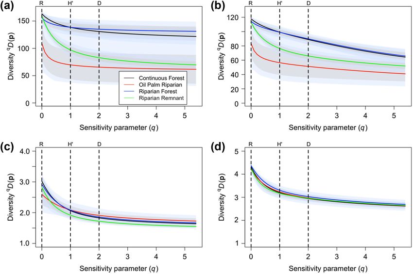
Keywords: biodiversity, diversity index, diversity profile, occupancy, presence, species distribution modeling, specificity, threshold

Introduction                                                         Cobbold 2012). Obtaining information on species abun-
                                                                     dance can, however, be challenging. Raw count data are
Biological diversity represents the variety of organisms or traits   typically fraught with detection bias (Nichols et al. 1998,
and plays a central role in ecological theory (Loreau et al.         MacKenzie and Kendall 2002, Sollmann et al. 2013), and
2001, Tilman et al. 2014). Mathematical functions known as           inference about diversity from indices based on count-
diversity indices aim to summarize properties of communi-            based relative abundance estimates that do not account for
ties that allow comparison among different regions, taxa and         imperfect and varying detectability may therefore be biased.
trophic levels (Morris et al. 2014, Daly et al. 2018). They          Estimating abundance of all species in a community while
are often used in conservation as indicators of the integrity        accounting for varying detection, for example using capture–
or stability of ecosystems, and are, therefore, of fundamental       recapture methods (Royle and Dorazio 2008), is extremely
importance for environmental monitoring and conservation             difficult as different organisms require different sampling
(Morris et al. 2014). Diversity is, however, a generic term          methods to obtain sufficient data for reliable abundance
describing the complex multidimensional properties of a              estimation. Thus, community studies often resort to the col-
community. Any diversity index reduces these multidimen-             lection of much cheaper and easier to obtain species detec-
sional properties to a single number (Morris et al. 2014),           tion/non-detection data. Even with these incidence data
which is problematic (Daly et al. 2018).                             we must consider that species may be detected imperfectly
    The most commonly used diversity indices are species             (MacKenzie et al. 2002, 2006).
richness, Shannon’s diversity H′ and Simpson’s diversity D;              Occupancy modelling provides a framework to handle the
the latter two combine measures of richness and abundance,           problem of imperfect and varying detection, producing unbi-
whereas species richness solely presents the number of spe-          ased estimates of species occurrence (MacKenzie et al. 2002,
cies. It is not uncommon that diversity increases according to       2006). The development of hierarchical multi-species occu-
one index, but decreases according to another (Patil 2014),          pancy models (Dorazio and Royle 2005, Dorazio et al. 2006)
demonstrating the difficulties in quantifying biodiversity in        has enabled estimation of richness at the level of the study
a single number (Purvis and Hector 2000, Daly et al. 2018).          area and survey location (Sollmann et al. 2017), and to model
    To address this shortcoming, several researchers have sug-       variation in richness across areas as a function of covariates
gested using parametric families of diversity indices (Hill          (Sutherland et al. 2016). However, it has been shown that
1973, Patil and Taillie 1982, Gattone and Battista 2009,             multi-species occupancy models overestimate true species
Leinster and Cobbold 2012). Jost (2006) proposed the use             richness (Zipkin et al. 2012), and only a few applications
of Hill numbers (Hill 1973) that incorporate relative abun-          for other diversity indices exist (Broms et al. 2016, Guillera-
dance and species richness to show the number of equally             Arroita et al. 2019). Consequently, accounting for imperfect
abundant species necessary to produce the observed value of          detection has often been neglected in calculating diversity
diversity. Individual Hill numbers differ by the parameter q,        metrics in the past.
which quantifies how much the measure discounts rare spe-                Only recently, Chao et al. (2014) described a method to
cies when calculating diversity (the higher q, the less these        calculate Hill numbers from incidence data, and Broms et al.
rare species contribute to diversity). Leinster and Cobbold          (2015) followed with a formulation to calculate detection-
(2012) further developed this framework to incorporate               corrected occupancy-based Hill numbers. Here, we extend
similarity between species and present them along a gradi-           this framework to facilitate the calculation, visualization, and
ent of q that includes Rao’s quadratic entropy and species           thus, interpretation of occupancy-based diversity profiles. We
richness. The naive similarity collapses diversity to the Hill       first explored how occupancy-based diversity profiles compare
number of order q (Hill 1973). Hill numbers include typical          to true abundance-based diversity profiles using simulated
diversity indices, where q = 0 reflects species richness, q = 1 is   data. Because of the asymptotic relationship between occu-
the exponential of the Shannon entropy and q = 2 represents          pancy and abundance (i.e. occupancy approaches 1 as abun-
the inverse of Simpson’s concentration. Plotting the effec-          dance increases, thus decreasing differences between species),
tive number of species as a function of q allows us to view          we expect occupancy-based profiles to overestimate diversity
diversity from multiple vantage points (Hill 1973, Leinster          for q > 0 (i.e. suggest a more even community). Moreover,
and Cobbold 2012) and the resulting curves have become               based on previous work (Zipkin et al. 2012, Broms et al.
known as diversity profiles. These curves display different          2016, Guillera-Arroita et al. 2019) we expect occupancy-
properties of diversity and often drop sharply between q = 0         based profiles to overestimate richness, due to characteris-
and q = 1 and level off soon after q = 2, indicating that many       tics of the underlying community occupancy models (see
communities are dominated by a few highly abundant species           ‘Occupancy threshold’ section for details) and that likely
(Preston 1948).                                                      inflates diversity at q > 0 as well. But because this affects all
    To calculate diversity indices (except for species richness),    communities, we expect occupancy-based profiles to still be
as well as diversity profiles, information about the relative        able to correctly order areas by their diversity. Therefore, we
abundances of species, or evenness, is required (Leinster and        tested their ability to compare communities across landscapes

2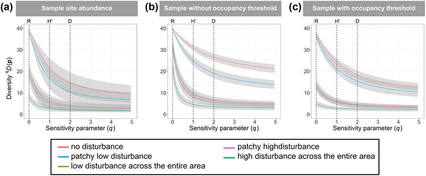
with varying levels of habitat disturbance, associated with of the performance of the occupancy-based diversity profiles
varying levels of diversity. We then used an empirical dataset by comparing them to true community abundance diver-
of diverse bird communities collected in Sabah, Malaysian sity profiles. In the second part of our study, we applied
Borneo, to demonstrate how the framework can be extended the community occupancy diversity profiles to an empirical
to a trait-based diversity analysis of occupancy-data by incor- bird dataset from Malaysian Borneo and demonstrate how
porating measures of similarity as proposed by Leinster and these profiles can account for phylogenetic or ecological trait
Cobbold (2012). similarities.
Forest degradation and community simulation
Methods
We simulated five virtual 10 × 10 km forest landscapes,
Our study was divided into a simulation study and an appli- with 200 × 200 m grid cells (50 × 50 cells). We simulated
cation of occupancy-based diversity profiles to an empirical a habitat covariate representing ‘habitat disturbance’ (where
dataset. The simulation study followed six steps: 1) simula- 0 represents undisturbed forest and 5 represents complete
tion of a forest degradation gradient, 2) simulation of animal deforestation) for each landscape (Fig. 1A) by drawing ran-
communities, and detection data of those communities, 3) dom samples from a multivariate normal distribution. To
community occupancy analysis of simulated detection data, increase realism by simulating nonrandom habitat, we explic-
4) utilization of community occupancy model output to con- itly included spatial autocorrelation in the simulation of the
struct occupancy-based diversity profiles, 5) application of habitat covariate by using the distance matrix as our variance-
thresholding to occupancy-based profiles and 6) evaluation covariance matrix and a decay function with a decay constant
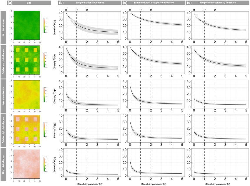
Figure 1. Results from the simulation study. (A) Simulated ‘forest quality’ habitat covariate for five virtual landscapes. Average diversity
profiles (solid line) for simulated data generated using data from only the 100 surveyed stations for (B) the simulated true abundance, and
the community occupancy predictions for the entire landscape (C) without thresholding and (D) with thresholding using the maxSSS
method for the entire study landscape, showing the standard deviation (grey shading).
3
ϕ to specify how the relationship to other cells changes with
distance (Supporting information). The five landscapes con-             ( )
                                                                   logit rijk = a0i       Detection probability
stitute a habitat degradation gradient representative of three
different logging regimes and two ‘patchy’ landscapes that         where yijk is the observed count data and rijk is the probability
simulate activities such as compartmental logging: 1) no dis-      of detection of an individual present at site j. We repeated the
turbance, 2) patchy low disturbance (i.e. low impact logging       observation process for 10 occasions, k. The average detec-
restricted to a few logging compartments), 3) low disturbance      tion probability for the community for all landscapes was set
across the entire area (i.e. low impact logging conducted          to 0.5. Species-specific intercepts for detection on the logit
throughout the logging concession), 4) patchy high distur-         scale, α0, were drawn from a normal distribution describing
bance (i.e. conventionally logging restricted to a few logging     the community (µα = 0, σα = 1).
compartments) and 5) high disturbance across the entire area          Finally, we reduced the observed count data y to detec-
(i.e. conventional logging conducted throughout the logging        tion/non-detection data. We chose to represent the detection
concession).                                                       process in two steps (generating counts, then reducing these
    We then simulated the cell-level abundance of 40 virtual       to binary detection/non-detection data) to reflect how data
species distributed within our five landscapes. We simulated       from typical non-invasive survey methods, such as bird point
abundance to generate true abundance-based diversity pro-          counts or camera-trapping, are prepared for occupancy mod-
files. Abundance was simulated for each of the 40 species, i, at   eling. We compared the performance of the occupancy-based
grid cell j (j = 1, 2,…nT) in each of our five landscapes under    diversity profiles to true community abundance diversity
the following model:                                               profiles. We repeated the simulation process to generate 100
                                                                   communities. All calculations were carried out in R ver. 3.6.0
                                                                   ().
                ( )
N ij ~ Poisson lij            True abundance
                                                                   Community occupancy model

    ( )
log lij = b0i + b1i ´ habitat j        Expected abundance
                                                                   We adopted the hierarchical formulation of occupancy models
                                                                   by Royle and Dorazio (2008) extended to a community occu-
                                                                   pancy model (Dorazio and Royle 2005, Dorazio et al. 2006).
where the species-specific intercepts (β0) and dependence          To analyze our simulated data, we combined data from all five
on the habitat covariate (β1) are simulated as normally dis-       landscapes and, following common practice in analyzing field
tributed with community hyperparameters (Supporting                data, modelled occupancy probability as having species-specific
information):                                                      random intercepts, β0is, with landscape specific (indicated by
                                                                   s indexing) hyperparameters (µβ0,s, σβ0,s), to allow for different
                (
b0i ~ Normal m0 , s02    )                                         baseline occupancy in the different landscapes and among spe-
                                                                   cies. We further modelled species-specific effects on occupancy
                                                                   of the simulated habitat ‘disturbance’ covariate (β1i). Detection
                                                                   probability included a species-specific random intercept with
               (
b1i ~ Normal m1 , s12   )                                          landscape specific hyperparameters, to allow for differences in
                                                                   baseline detection among landscapes. In our case, the different
                                                                   landscapes had different abundances of animals, which leads
We set the average response of species to habitat disturbance      to differences in species-level detection (Royle and Nichols
as negative (µ1 = −2) since most forest-adapted species will       2003) and likely also to differences in species-level baseline
respond to logging negatively (Supporting information).            occupancy probability. When fewer than the 40 simulated
We allowed this to vary, generating a community of species         species were observed across all landscapes, we augmented the
with mostly negative responses, but with few species that          observed data set with 40 minus the number of observed spe-
responded positively to habitat disturbance. Average expected      cies with all-0 detection data (note that this implies more data
abundance per species per grid cell in undisturbed forests was     augmentation, and thus a higher potential for positive bias in
0.37. This resulted in five communities with species richness      diversity estimates, in more disturbed landscapes with fewer
ranging from 17.2 (± 2.8) for the most disturbed site to 40        species, compared to less disturbed landscapes where more
(± 0) for the undisturbed site.                                    species were present). The formal model description can be
    We then generated detection/non-detection data by simu-        found in the Supporting information. We implemented the
lating systematic repeated sampling of the community. For          model in a Bayesian framework using JAGS (Plummer 2003)
each landscape, we picked 100 sampling points in a grid            accessed via the R packages rjags (Plummer 2019). We ran
spaced 2 km apart. At each point, we then simulated the            three parallel Markov chains with 250 000 iterations, of which
observation process with imperfect detection:                      we discarded 50 000 as burn-in, and we thinned the remain-
                                                                   ing iterations by 20 to make the output more manageable. We
                                                                   assessed chain convergence using the Gelman–Rubin statistic
                    (
yijk ~ Binomial N ij , rijk   )   Observed count data              (Gelman et al. 2004). Values under 1.1 indicate convergence,

4
and all parameters in our models had a Gelman–Rubin statis- æ ö
( Z y )i = å h =1Zih çç Sy( yh ) ÷÷
M
tic < 1.1. We tested whether the model adequately fit the data (4)
by calculating a Bayesian p-value (Gelman et al. 1996). We è ø
observed no lack of fit for any of our models. where M is again the number of species in the assemblage,
Diversity profiles yi is the average occupancy probability of species i, the ith
yi
species has relative occupancy and Z is the similar-
In order to investigate the performance of estimating diver- S (y )
sity profiles with occupancy-based information, we first ity matrix. This adjustment is similar to that developed by
constructed diversity profiles for the simulated abundance Broms et al. (2015) but extends their approach by allow-
across the sampling stations. Diversity profile values (qDZ) for ing occupancy probability to be modeled as a function of
abundance data can be calculated according to Leinster and covariates.
Cobbold (2012) as: We used the parameter estimates from the occupancy
model fit to our simulated data to calculate species occupancy
1 for the sample stations in the five simulated landscapes and
æ li ö1-q then constructed diversity profiles using the mean occupancy
å
M
q
DZ | l = ç
ç i =1 S ( l )
( Z l )iq -1 ÷÷ (1) probability across sampling stations for each species using Eq.
è ø 3 and 4 for all posterior samples of the community occupancy
where model. This effectively creates posterior distributions for the
diversity profiles themselves and allowed us to determine
their standard deviations (SDs) and 95% Bayesian credible
æ lh ö
( Z l )i = å h =1Z ih çç
M
÷÷ (2) intervals. We then compared estimates of R, H′ and D from
è S (l) ø the occupancy-based profiles against indices based on the
true abundance profiles by evaluating the diversity profiles at
where λ represents abundance, M is the number of species q = 0, q = 1 and q = 2, respectively. Specifically, for each land-
in lthe assemblage and the ith species has relative abundance scape, we present the average relative bias (occupancy-based
i
. The parameter q determines the sensitivity of the mea- index minus true abundance index divided by true index)
S ( to) the relative abundances of species. This allows us to cal-
sure l across all 100 communities and coverage, i.e. the proportion
culate diversity along a continuum of values of q. At q = 0, qDZ of communities for which the 95% CI of the occupancy-
equals species richness where all species are considered equally. based index estimate included the true-abundance based
As q becomes larger, more weight is placed on common species index. We also generated occupancy-based diversity pro-
thereby incorporating evenness into the diversity measure and files for landscape wide predictions of occupancy generated
resulting in a lower value of qDZ for more uneven assemblages using the parameters estimated in the community occupancy
than for more even assemblages. The diversity profile frame- model. We did this to compare the results between the sam-
work from Leinster and Cobbold (2012) allows for the consid- pling station-based profiles and the landscape-wide profiles.
eration of similarity between species through the inclusion of To evaluate how well occupancy-based diversity profiles
an M × M similarity matrix Z which represents the similarity were able to order landscapes by site diversity rank, we com-
between the ith and hth species. Values of 0 in Z indicate total pared them to the diversity ranking in the true abundance-
dissimilarity, whereas values of 1 indicate identical species. This based profiles. Since not all communities were different in
matrix can be used to adjust the profiles by incorporating any the true abundance-based profiles (e.g. no disturbance and
measure of similarity (such as phylogenetic or trait) between patchy low disturbance landscapes both had an average spe-
different species or taxonomic groups. In our simulation study, cies richness of 40 (Supporting information) and could,
we use a naive similarity matrix (an identity matrix with all therefore, not be distinguished in the true-abundance based
cells on the diagonal equal to 1 and all other values = 0). In the profiles), we first determined how many sites we could reli-
empirical dataset (below) we adjusted the profiles using a diet, ably distinguish. To do so we used the results of the true
taxonomic and a phylogenetic similarity matrix. We refer to abundance-based simulations and checked which landscapes
q = 0 as ‘richness’ (R), which, depending on the nature of Zih, could be distinguished in 95% of the 100 simulations for R,
can represent species richness, or trait richness. H′ and D. We were able to distinguish between 3, 4 and 3
To use occupancy probabilities instead of abundances to of the 5 sites in the true abundance profiles for R, H′ and D,
construct diversity profiles we altered the diversity profile respectively (Supporting information). We then calculated
method of Leinster and Cobbold (2012) as follows: the proportion of communities for which occupancy-based
diversity profiles resulted in the same rank order of these dis-
1
tinguishable landscapes as true abundance-based profiles.
æ yi q -1 ö1- q
å ( )i
M
q
DZ | y = ç Z ÷÷ (3) Occupancy threshold
ç i =1 S (y) y
è ø
Community occupancy models have been shown to over-
where estimate diversity through several processes: when data
5Table 1. Percentage of the 100 simulated communities within each of five landscapes where occupancy-based diversity profiles were
ordered the same as the true abundance-based diversity profiles. The maximum number of landscapes that could be reliably separated in
the true abundance profiles was 3, 4 and 3 of the 5 landscapes for R, D and H′, respectively (Supporting information).
Landscape-wide Landscape-wide occupancy Sample-station Sample-station occupancy
Index occupancy with threshold occupancy with threshold
Species richness (R, q = 0) 97% 100% 97% 100%
Shannon diversity (H′, q = 1) 96% 94% 96% 92%
Simpson’s index (D, q = 2) 94% 90% 94% 82%
augmentation is used to estimate richness including species Case study
never observed, it induces a non-0 probability of occurrence
for augmented species, which can inflate richness (and likely We sampled bird communities at 307 point-count locali-
other diversity) estimates. Further, because rare species bor- ties in and around the Stability of altered forest ecosystems
row information from common species (through shared (SAFE) project (117°5'N, 4°6'E) in Sabah, Malaysian
hyperparameters), their occupancy probability may be over- Borneo (Mitchell et al. 2018). Thirty-eight localities were
estimated (Broms et al. 2016, Guillera-Arroita et al. 2019). in continuous logged forest (CF) of the Ulu Segama Forest
Finally, for data sparse species, detection probability may be Reserve, with an additional 156 in the neighboring SAFE
underestimated, and occurrence probability consequently landscape, in forest that had been logged several times and
overestimated, which has been shown to lead to positive bias recently salvage logged. A further 113 localities were sampled
in occupancy-based Hill numbers (Broms et al. 2015). To alongside rivers in oil palm plantations, including 88 with
explore methods to account for the expected overestima- riparian forest remnants (RR) on each riverbank and 15 with
tion of diversity profiles in community occupancy models, no natural vegetation (OPR). Localities are classified by habi-
we tested the use of an occupancy threshold. An occupancy tat into four categories: non-riparian continuous forest (CF),
threshold is traditionally used to transform occupancy prob- riparian forest (RF), riparian remnant (RR) and oil palm river
abilities into binary outputs. Here, we explore the use of a (OPR). Forest quality, based on aboveground carbon den-
threshold to determine at which occupancy levels we can sity measured via LiDAR, also varied substantially across the
consider a species to truly occupy a landscape, thus reducing landscape.
the overestimation in richness. Point counts were undertaken by a single experienced
When using presence/absence data, the identities of observer (SLM) for 15 min on mornings without rain, record-
both presence and absence data are (assumed to be) known ing all birds heard or seen within a 50-m radius. Each point
(Liu et al. 2016). However, with detection/non-detection was sampled three times, typically within a few weeks, dur-
data we have no information about ‘true absences’, which ing field work undertaken 2015–2018 (for details, Mitchell
presents challenges for threshold selection. Liu et al. (2016) et al. 2018).
identified the maxSSS method, which maximizes the sum We observed a total of 169 bird species. Two species,
of sensitivity and specificity, as the most suitable objective Leptocoma brasiliana and Zanclostomus javanicus, were
approach for determining thresholds with incidence data excluded because there is no phylogenetic information avail-
(presence-only data). able, which is necessary for the trait-based analysis. Further,
The maxSSS method described by Liu et al. (2016) requires three species of swift (Aerodramus maximus, A. salangana and
the use of ‘pseudo-absences’, which are randomly picked A. fuciphagus) could not be reliably separated and are consid-
from the sampling stations with no detections. Here, we use ered as Aerodramus spp.
the estimates from the occupancy model to draw ‘pseudo- To analyze the case study data, we used a similar com-
absences’ randomly for stations without detections but munity occupancy model structure as used for the simulation
weighed by the probability of a station being unoccupied, study. Following Mitchell et al. (2018), we modeled occu-
1 − ψ. pancy using above-ground carbon density, forest cover and
We calculated the maxSSS (Supporting information) thresh- riparian remnant width as predictors, with species-specific
old for each species for each landscape based on the mean random intercepts with habitat-specific hyperparameters.
occupancy estimate using the optimal.thresholds function Covariates were derived using remotely sensed data and cal-
from the R package PresenceAbsence (Freeman and Moisen culated following Mitchell et al. (2018). Detection probabil-
2008). We set occupancy probabilities for stations with esti- ity included a species-specific random intercept with habitat
mates below the occupancy threshold to zero. We then aver- specific hyperparameters and accounted for the effect of time
aged the threshold-adjusted occupancy for each species across and date of a survey on the probability of detection (Ellis and
landscapes for each model iteration and generated new diver- Taylor 2018).
sity profiles using the adjusted dataset. We compared thresh- We separated species communities according to the four
old occupancy-based profiles against true-abundance based habitat-types described above for diversity profile construc-
profiles as described for non-threshold profiles and evaluate if tion with and without occupancy thresholds. We used the
using a threshold improves our ability to distinguish between occupancy probabilities for each sampling station to con-
the landscapes. struct the diversity profiles. Additionally, we constructed
6similarity matrices according to diet, taxonomy and phylog- information). Applying the threshold reduced positive bias
eny (Supporting information) to demonstrate how similar- and improved coverage of diversity for q > 0, but resulted in a
ity can be incorporated into the occupancy-based diversity negative bias and poorer coverage of species richness, particu-
profile framework. larly in more disturbed landscapes (Supporting information).
For both abundance and occupancy-based profiles, we did
not find great discrepancies between the sampling station-
Results based profiles and the landscape-wide profiles, even though
the sampling stations only covered about 4% of the study area
Simulation results (for landscape wide profiles see the Supporting information).
For the comparison across landscapes the occupancy-
The number of species present in the simulated true abun- based diversity profiles generally maintained the same rank
dance data in each landscape ranged between, on average, order of diversity amongst the landscapes (Fig. 2A, for an
17 and 40, whereas the number of species detected in each example of results from a single site see the Supporting infor-
landscape ranged between, on average, 8 and 39, indicating mation) as the abundance-based diversity profiles. The three
that our simulation of the detection process resulted in the communities that showed significantly different species rich-
detection of between 47 and 99% of the species present in ness based on true abundance data were ordered the same by
the five landscapes. On average across the five landscaped, six occupancy-based richness estimates in 97% of the simulated
species were missed due to imperfect detection. We present communities (Fig. 2B, Table 1). Similarly, the four and three
the average and standard deviation (as a measure of variability landscapes that could be significantly distinguished for H′
among simulated communities) for the true abundance and and D were ordered the same as occupancy-based profiles in
occupancy-based profiles generated for the sample stations in 96% and 94% of all simulations, respectively. The occupancy
100 simulated communities in Fig. 1. The occupancy-based threshold slightly increased the ability to correctly rank simu-
diversity profiles (Fig. 1C without thresholding and Fig. 1D lated landscapes by species richness (to 100%), but slightly
with the threshold, for the application of this method to a sin- reduced it for H′ and D (Fig. 2C, Table 1).
gle site see the Supporting information) showed similar trends
in diversity as the diversity profiles based on true abundance Borneo bird community results
(Fig. 1B). Occupancy-based species richness estimates without
thresholding corresponded well to true richness for all but the We detected 143, 118, 121 and 30 species in continuous
most disturbed landscape (average bias of 38%). As expected, forest, riparian forest, riparian remnant and oil palm river,
for q > 0.5 (including H′ and D), occupancy-based diversity respectively. In the diversity profiles, species richness was
profiles showed consistent positive bias (Fig. 1B, Supporting highest in continuous forest, followed by (in decreasing
information). Patterns in coverage mirrored patterns in bias, order) riparian remnant, riparian forest and oil palm river.
with nominal (> 95%) coverage of richness, but poor cover- At q < 1, continuous forest was the most diverse habitat
age (between 0 and 27%) of the other two indices (Supporting type, while at q > 1.5 riparian forest was the most diverse
Figure 2. Comparison among landscapes of diversity profiles generated using (A) the true abundance at the 100 sample stations in each
landscape, (B) occupancy based predictions at the 100 sample stations in each landscape without thresholding, (C) occupancy based predic-
tions at the 100 sample stations in each landscape with thresholding. All results are shown as averages (solid line) of the 100 simulations
with the uncertainty shown as standard deviations (grey shading).
7(Fig. 3A), although the 95% CIs of the profiles for these communities in the riparian remnant and the oil palm river,
two more diverse habitats overlapped. Although species were less distinct.
richness in the riparian remnant was similar to continu-
ous forests and riparian forest, the diversity decline of the
profile was much greater, so that riparian remnants were Discussion and conclusion
significantly (non-overlapping 95% CIs) distinct from con-
tinuous forest and riparian forest at q > 0.5. Oil palm river Diversity profiles allow researchers to characterize and com-
and riparian remnant were always the habitats with the pare communities while considering the contributions of
lowest and second lowest biodiversity, respectively, and at abundant and rare species, thus acknowledging the mul-
q > 2 the 95% CIs of these two profiles largely overlapped. tidimensional nature of diversity (Morris et al. 2014).
When we incorporated similarity (diet, taxonomic and Occupancy-based diversity profiles provide a reliable infer-
phylogenetic), the overall community diversity was reduced ence framework for estimating biodiversity based on output
for all habitat types. In line with species richness, the taxo- from community occupancy models, which take into account
nomic richness (Fig. 3C) was similar for the riparian remnant, imperfect and varying species detection. As expected, we
continuous forest and riparian forest. Continuous forest and found that occupancy-based diversity profiles generally mir-
riparian forest showed very similar overlapping profiles. The rored true among-community patterns well, albeit with some
shape of the riparian remnant and oil palm river taxonomic shortcomings that are primarily related to overestimations of
profiles were very similar to the original profiles but overlap non-richness diversity measures.
in the 95% CIs was even greater. When we considered dietary Using occupancy model estimates of average occupancy
(Fig. 3B) and phylogenetic (Fig. 3D) similarity, we also saw a probability to construct diversity profiles, with or without
large reduction in the diversity of the communities. In both thresholding, generally maintained the same inter-landscape
cases, all habitats showed very similar diversity profiles with diversity pattern as observed in the true abundance diversity
widely overlapping 95% CIs. profiles (Fig. 2). Further, the two simulated landscapes that
With thresholding (Supporting information), the esti- had very similar abundance-based profiles (landscape-wide
mated species richness was lower for all habitat types. low disturbance and local high disturbance) also showed
Profiles with the threshold showed similar patterns, but dif- very similar occupancy-based profiles. The general agreement
ferences among habitats, particularly for the more depleted of the occupancy and true abundance profiles suggests that
Figure 3. Diversity profiles for a bird community from Malaysian Borneo in four habitat types calculated using the occupancy predictions
without thresholding. (A) Naive similarity matrix, (B) taxonomic similarity, (C) diet similarity, (D) phylogenetic similarity. The standard
deviations (grey shading) and 95% credible intervals (blue shading) are included to quantify uncertainty.
8detection/non-detection surveys may be sufficient to com- our ability to correctly replicate true underlying differences
pare the multidimensional properties of diversity between in diversity among landscapes (Table 1). In the empirical
landscapes. Similarly, the repeated collection of detection/ dataset, we saw a similar reduction in the distinctiveness of
non-detection data from one landscape will likely allow com- diversity profiles for the riparian remnants and the oil palm
parison of diversity through time, an important aspect of bio- rivers, whose 95% CIs largely overlapped for q > 1 when a
diversity monitoring. threshold was applied. As we expect that the main objective
Within a landscape, occupancy-based profiles generally of most biodiversity research and monitoring projects is the
overestimated diversity for q > 0. This is expected because comparison of profiles between sites or of the same site across
occupancy approaches 1 as abundance increases; conse- time, we recommend to not use the threshold we applied. In
quently, occupancy-based diversity should suggest more even this case, researchers should be aware that species richness
communities (i.e, be higher) than abundance-based diversity. and potentially entire diversity profiles may be overestimated
Further, Broms et al. (2015) also found positive bias when when detection is low for many species. We acknowledge that
comparing their occupancy-based to true incidence-based we only explored one threshold and that effects may be differ-
Hill numbers and attributed that to positively biased esti- ent for other threshold methods; this is an avenue for future
mates of occupancy in species with low detection rates. This development of this approach.
bias is caused by the structure of the community occupancy Acknowledging the differences between abundance and
framework, as rare species borrow information from common occupancy, we do not suggest that occupancy probability can
species (Broms et al. 2016, Guillera-Arroita et al. 2019), and simply be used as an index or surrogate for abundance. Our
may also contribute to the positive bias we observed. Similar results do, however, indicate that occupancy-based diversity
to Broms et al. (2015), we saw no or low negative bias in esti- measures and profiles can reflect patterns in diversity despite
mates of species richness (q = 0), with exception of the most the loss of information entailed in using occupancy rather
disturbed landscape, which had 33.8% positive bias in rich- than abundance data. This is a promising finding for bio-
ness estimates, on average. Several factors likely contribute to diversity research and monitoring, as community-wide spe-
this positive bias: First, the rarity of many of the species in cies detection/non-detection data are generally much easier
this landscape translates into low species detection probabili- and cheaper to obtain than data for abundance estimation
ties and thus, likely positive bias in occupancy, as explained (Joseph et al. 2006, Kéry and Schmidt 2008). In addition
above. Second, our approach to analyze data from all land- to traditional methods used to detect wildlife, such as points
scapes combined implies augmenting data for the most dis- counts and visual transects, a growing number of technolo-
turbed site with a large number of all-0 encounter histories gies are available for detecting and identifying biodiversity,
(reflecting the implicit assumption that all species from such as automated acoustic recorders (Bush et al. 2017) or
the regional pool could potentially occur in the disturbed eDNA and metabarcoding (Bush et al. 2017). These new
landscapes). Occupancy probability for these species, even technologies present powerful methods to collect community
if low, is non-0, and thus contributes to richness estimates. level detection/non-detection data that could be combined
The potential for this source of bias is lower in landscapes with occupancy-based diversity profiles.
where true richness is closer to the 40-species threshold. As an It is important to note that with an average detection
alternative, we could have analyzed data from each landscape probability of 0.5 and 10 sampling occasions, our simulated
separately, conditioning on the number of species observed in data represent a scenario where most species in a community
each landscape. That, however, would have induced negative are detected. These conditions are representative of typical
bias in richness (and possibly other diversity) estimates, as camera-trap surveys in which the number of possible repeat
not all species present were always observed. visits is much less limited by logistics than methods requir-
We attempted to overcome the overestimation of diver- ing a human observer to return to each sampling location
sity from community occupancy models by implementing an on each occasion (e.g. point counts). Based on our findings
occupancy threshold. Liu et al. (2016) suggest the use of ran- for the most disturbed landscape (e.g. strong positive bias in
domly selected points as pseudo-absences for threshold deter- richness estimates from community occupancy models), we
mination with incidence data. Here, we used the output of expect sparser data from surveys with lower species detectabil-
the occupancy model to generate pseudo-absences based on ity and/or fewer repeated visits to increase the potential for
estimated occupancy probability. This approach likely leads positive bias in diversity profiles. Further studies are needed
to more realistic pseudo-absences than completely random to explore the effects of varying p and k on occupancy-based
generation as the use of modeled occupancy probabilities diversity profiles.
allows for a more informed selection. Incorporating a thresh- The diversity profile framework presented here also allows
old into occupancy-based diversity profile calculation had for the incorporation of trait similarities between species
mixed results. The threshold reduced the overestimation of by defining a similarity matrix. Incorporating species trait
diversity at q > 0.5 (Supporting information). At the same similarities can be an additional way to display diversity in
time, however, thresholding often resulted in underestimated a community as it puts a greater emphasis on more dissimi-
species richness, particularly for more disturbed landscapes lar species (Leinster and Cobbold 2012). From an ecological
(Supporting information) for q > 0. Interestingly, the use perspective, accounting for such similarities reduces the func-
of a threshold did not improve, but rather slightly reduced tional redundancies in the community, for example, species
9having the same dietary niche could functionally replace each species detection probability to estimate local abundance
other (Rosenfeld 2002, Olden et al. 2004). Phylogenetically from detection/non-detection data. At the same time, our
and functionally diverse communities are known to better results highlights that even a basic community occupancy
maintain ecosystem stability (Cadotte et al. 2011, 2012). model will in most cases be sufficient to compare different
Therefore, considering these additional dimensions of sites in terms of diversity.
diversity provides a more complete picture of a community In practice, information on species occurrence is often
(Rodrigues and Gaston 2002) and may improve predictions used to help develop management decisions and conser-
of ecosystem function and resilience. vation strategies (Guisan et al. 2013). For many species of
Our empirical data showed that considering dietary, taxo- conservation concern, the detection/non-detection surveys
nomic or phylogenetic similarities among bird species led to underlying estimates of occurrence are the main source of
very similar diversity profiles for all habitat types. In the case information on their population status, and therefore have a
of this bird dataset, all taxonomic, phylogenetic and dietary significant role in setting conservation priorities (MacKenzie
groups were present in all habitats. As a result, even at con- 2005, Joseph et al. 2006). They are useful for a wide range of
siderably lower species diversity, disturbed habitats such as oil purposes from estimating changes in occurrence to identify-
palm plantations maintained dietary and phylogenetic diver- ing high conservation priority areas (Zipkin et al. 2010, Olea
sity of birds essentially identical to that of continuous for- and Mateo-Tomas 2011, Tilker et al. 2020). Occupancy-
ests. This is surprising, given that previous studies have found based diversity profiles are an important contribution to the
that dietary traits and taxonomy (among other characteris- occupancy toolkit as they allow comparing biodiversity across
tics) can affect response to habitat alterations and extinction space and time while accounting for imperfect and varying
risk in birds (Russell et al. 1998, Boyer 2010, Frishkoff et al. detection. Specifically, these profiles can be used to: 1) moni-
2014). Despite this apparent maintenance of phylogenetic tor the diversity of a community over time and to evaluate
and functional diversity, the loss of overall species diversity in the effectiveness of management/conservation efforts, and 2)
more disturbed habitats suggest a loss in redundancy, another compare general patterns of diversity according to different
measure that has been associated with ecosystem stability habitat, disturbance or trait regimes, helping to set conser-
(Naeem 1998). vation priorities. Incorporating this approach into conserva-
The diversity profiles of the bird communities reinforced tion should improve biodiversity assessments of species and
the findings by Mitchell at el. (2018) that riparian remnants communities.
supported similar diversity value to continuous logged for-
est habitats (both riparian and non-riparian). However, when Data availability statement
evenness of the community is given more weight (i.e. when
q > 1), riparian remnants have reduced diversity compared to Scripts and model code are available on github (). For access to the
habitat remnants (such as when measured via species richness data used in this study please contact the corresponding
directly), manifests from a number of species occurring rarely. author.
If a greater proportion of the community in remnant occurs
only rarely, this suggests such remnants may not sustain cer-
tain species in the long-term (i.e. we may be observing an Acknowledgements – We thank the German Federal Ministry
extinction debt) and effectively act as population sinks from of Education and Research (BMBF FKZ: 01LN1301A; FKZ:
continuous forest habitats, a finding which is not apparent 01LC1703A) and the Leibniz Institute for Zoo and Wildlife
from assessing only species richness and community integrity Research for funding this research. SLM and MJS were funded
as undertaken by Mitchell et al. (2018). by the UK Natural Environment Research Council (NERC: NE/
K016407/1). SLM was supported by a PhD scholarship jointly
Beyond exploring alternative threshold approaches and
funded by University of Kent and NERC. We thank the Sabah
the effects of sample size on occupancy-based diversity pro- Biodiversity Council, Sabah Forest Department, Yayasan Sabah,
files, there are several opportunities to further develop the Sime Darby, Benta Wawasan, Sabah Softwoods and Innoprise
application of detection-corrected diversity profiles to typical Foundation for permitting site access. We are grateful to David
wildlife survey data. We focused on detection/non-detection Coombs and Tom Swinfield for providing LiDAR data used as
data as these are the most easily collected for communities covariates in the occupancy model. Open access funding enabled
of difficult-to-study species (though ‘easy’ is a relative term). and organized by Projekt DEAL.
When repeated count data are available, as is often the case Conflict of interest – The authors declare no conflict of interests.
for bird surveys, a community N-mixture model (Royle 2004,
Yamaura et al. 2016) could be used to construct detection- Author contributions
corrected abundance-based diversity profiles. Distance sam-
pling data on a community of species (Sollmann et al. 2016) Jesse F. Abrams: Conceptualization (equal); Data cura-
could be used for that same purpose. Even with species-level tion (equal); Formal analysis (lead); Methodology (equal);
detection/non-detection data, researchers could employ the Visualization (lead); Writing – original draft (lead);
Royle–Nichols occupancy model (Royle and Nichols 2003), Writing – review and editing (equal). Rahel Sollmann:
which exploits the relationship between abundance and Conceptualization (equal); Formal analysis (supporting);
10Methodology (supporting); Writing – original draft (sup- Jost, L. 2006. Entropy and diversity. – Oikos 113: 363–375.
porting); Writing – review and editing (equal). Simon L. Kéry, M. and Schmidt, B. R. 2008. Imperfect detection and its
Mitchell: Data curation (equal); Writing – original draft (sup- consequences for monitoring for conservation. – Commun.
porting); Writing – review and editing (equal). Matthew J. Ecol. 9: 207–216.
Stuebig: Funding acquisition (lead); Writing – original draft Leinster, T. and Cobbold, C. A. 2012. Measuring diversity: the
importance of species similarity. – Ecology 93: 477–489.
(supporting); Writing – review and editing (equal). Andreas Liu, C. et al. 2016. On the selection of thresholds for predicting
Wilting: Conceptualization (equal); Formal analysis (sup- species occurrence with presence-only data. – Ecol. Evol. 6:
porting); Funding acquisition (lead); Writing – original draft 337–348.
(supporting); Writing – review and editing (equal). Loreau, M. et al. 2001. Biodiversity and ecosystem functioning:
current knowledge and future challenges. – Science 294:
804–808.
References MacKenzie, D. I. 2005. What are the issues with presence–absence
data for wildlife managers? – J. Wildl. Manage. 69: 849–860.
Boyer, A. G. 2010. Consistent ecological selectivity through time MacKenzie, D. I. and Kendall, W. L. 2002. How should detection
in Pacific island avian extinctions. – Conserv. Biol. 24: 511–519. probability be incorporated into estimates of relative abun-
Broms, K. M. et al. 2015. Accounting for imperfect detection in dance? – Ecology 83: 2387–2393.
Hill numbers for biodiversity studies. – Methods Ecol. Evol. 6: MacKenzie, D. I. et al. 2002. Estimating site occupancy rates when
99–108. detection probabilities are less than one. – Ecology 83:
Broms, K. M. et al. 2016. Model selection and assessment for 2248–2255.
multi-species occupancy models. – Ecology 97: 1759–1770. MacKenzie, D. I. et al. 2006. Occupancy estimation and modeling:
Bush, A. et al. 2017. Connecting Earth observation to high- inferring patterns and dynamics of species occurrence. – Aca-
throughput biodiversity data. – Nat. Ecol. Evol. 1: 0176. demic Press.
Cadotte, M. W. et al. 2011. Beyond species: functional diversity Mitchell, S. L. et al. 2018. Riparian reserves help protect forest bird
and the maintenance of ecological processes and services. – J. communities in oil palm dominated landscapes. – J. Appl. Ecol.
Appl. Ecol. 48: 1079–1087. 55: 2744–2755.
Cadotte, M. W. et al. 2012. Phylogenetic diversity promotes eco- Morris, E. K. et al. 2014. Choosing and using diversity indices:
system stability. – Ecology 93: S223–S233. insights for ecological applications from the German Biodiver-
Chao, A. et al. 2014. Rarefaction and extrapolation with Hill num- sity Exploratories. – Ecol. Evol. 4: 3514–3524.
bers: a framework for sampling and estimation in species diver- Naeem, S. 1998. Species redundancy and ecosystem reliability. –
sity studies. – Ecol. Monogr. 84: 45–67. Conserv. Biol. 12: 39–45.
Daly, A. et al. 2018. Ecological diversity: measuring the unmeasur- Nichols, J. D. et al. 1998. Inference methods for spatial variation
able. – Mathematics 6: 119. in species richness and community composition when not all
Dorazio, R. M. and Royle, J. A. 2005. Estimating size and compo- species are detected. – Conserv. Biol. 12: 1390–1398.
sition of biological communities by modeling the occurrence of Olden, J. D. et al. 2004. Ecological and evolutionary conse-
species. – J. Am. Stat. Assoc. 100: 389–398. quences of biotic homogenization. – Trends Ecol. Evol. 19:
Dorazio, R. M. et al. 2006. Estimating species richness and accu- 18–24.
mulation by modeling species occurrence and detectability. – Olea, P. P. and Mateo-Tomas, P. 2011. Spatially explicit estima-
Ecology 87: 842–854. tion of occupancy, detection probability and survey effort
Ellis, M. V. and Taylor, J. E. 2018. Effects of weather, time of day needed to inform conservation planning. – Divers. Distrib.
and survey effort on estimates of species richness in temperate 17: 714–724.
woodlands. – Emu-Austral Ornithol. 118: 183–192. Patil, G. P. 2014. Diversity profiles. – In: Balakrishnan, N. et al.
Freeman, E. A. and Moisen, G. 2008. PresenceAbsence: an R package (eds), Wiley StatsRef: statistics reference online. Wiley.
for presence–absence model analysis. – J. Stat. Softw. 23: 1–31. Patil, G. P. and Taillie, C. 1982. Diversity as a concept and its
Frishkoff, L. O. et al. 2014. Loss of avian phylogenetic diversity in measurement. – J. Am. Stat. Assoc. 77: 548–561.
neotropical agricultural systems. – Science 345: 1343–1346. Plummer, M. 2003. JAGS: a program for analysis of Bayesian
Gattone, S. A. and Battista, T. D. 2009. A functional approach to graphical models using Gibbs sampling. – In: Proc 3rd Int.
diversity profiles. – J. R. Stat. Soc. Ser. C 58: 267–284. workshop on distributed statistical computing, pp. 20–22.
Gelman, A. et al. 1996. Posterior predictive assessment of model .
fitness via realized discrepancies. - Stat. Sin. 6: 733-760. Plummer, M. 2019. rjags: Bayesian graphical models using MCMC.
Gelman, A. et al. 2004. Bayesian data analysis. - Chapman and – R package ver. 4-9.
Hall. Preston, F. W. 1948. The commonness, and rarity, of species. –
Guillera-Arroita, G. et al. 2019. Inferring species richness using Ecology 28: 254–283.
multispecies occupancy modeling: estimation performance and Purvis, A. and Hector, A. 2000. Getting the measure of biodiversity.
interpretation. – Ecol. Evol. 9: 780–792. – Nature 405: 212.
Guisan, A. et al. 2013. Predicting species distributions for conserva- Rodrigues, A. S. and Gaston, K. J. 2002. Maximising phylogenetic
tion decisions. – Ecol. Lett. 16: 1424–1435. diversity in the selection of networks of conservation areas. –
Hill, M. O. 1973. Diversity and evenness: a unifying notation and Biol. Conserv. 105: 103–111.
its consequences. – Ecology 54: 427–432. Rosenfeld, J. S. 2002. Functional redundancy in ecology and con-
Joseph, L. N. et al. 2006. Presence–absence versus abundance data servation. – Oikos 98: 156–162.
for monitoring threatened species. – Conserv. Biol. 20: Royle, J. A. 2004. N-mixture models for estimating population size
1679–1687. from spatially replicated counts. – Biometrics 60: 108–115.
11Royle, J. A. and Dorazio, R. M. 2008. Hierarchical modeling and Sutherland, C. et al. 2016. A multiregion community model for
inference in ecology. – Academic Press. inference about geographic variation in species richness. –
Royle, J. A. and Nichols, J. D. 2003. Estimating abundance from Methods Ecol. Evol. 7: 783–791.
repeated presence–absence data or point counts. – Ecology 84: Tilker, A. et al. 2020. Identifying conservation priorities in a defau-
777–790. nated tropical biodiversity hotspot. – Divers. Distrib. 26: 426–440.
Russell, G. J. et al. 1998. Present and future taxonomic selectivity Tilman, D. et al. 2014. Biodiversity and ecosystem functioning.
in bird and mammal extinctions. – Conserv. Biol. 12: – Annu. Rev. Ecol. Evol. Syst. 45: 471–493.
1365–1376. Yamaura, Y. et al. 2016. Study of biological communities subject
Sollmann, R. et al. 2013. Risky business or simple solution–relative to imperfect detection: bias and precision of community
abundance indices from camera-trapping. – Biol. Conserv. 159: N-mixture abundance models in small-sample situations. –
405–412. Ecol. Res. 31: 289–305.
Sollmann, R. et al. 2016. A hierarchical distance sampling model Zipkin, E. F. et al. 2010. Multi-species occurrence models to eval-
to estimate abundance and covariate associations of species and uate the effects of conservation and management actions. –
communities. – Methods Ecol. Evol. 7: 529–537. Biol. Conserv. 143: 479–484.
Sollmann, R. et al. 2017. Quantifying mammal biodiversity co- Zipkin, E. F. et al. 2012. Evaluating the predictive abilities of com-
benefits in certified tropical forests. – Divers. Distrib. 23: munity occupancy models using AUC while accounting for
317–328. imperfect detection. – Ecol. Appl. 22: 1962–1972.
12You can also read