LOCAL TESTS FOR IDENTIFYING ANISOTROPIC DIFFUSION AREAS IN HUMAN BRAIN WITH DTI
←
→
Page content transcription
If your browser does not render page correctly, please read the page content below
The Annals of Applied Statistics
2013, Vol. 7, No. 1, 201–225
DOI: 10.1214/12-AOAS573
© Institute of Mathematical Statistics, 2013

     LOCAL TESTS FOR IDENTIFYING ANISOTROPIC DIFFUSION
              AREAS IN HUMAN BRAIN WITH DTI

              B Y TAO Y U1 , C HUNMING Z HANG2 , A NDREW L. A LEXANDER3
                               AND R ICHARD J. DAVIDSON 3

National University of Singapore, University of Wisconsin-Madison, University of
           Wisconsin-Madison and University of Wisconsin-Madison
                      Diffusion tensor imaging (DTI) plays a key role in analyzing the physi-
                 cal structures of biological tissues, particularly in reconstructing fiber tracts
                 of the human brain in vivo. On the one hand, eigenvalues of diffusion ten-
                 sors (DTs) estimated from diffusion weighted imaging (DWI) data usually
                 contain systematic bias, which subsequently biases the diffusivity measure-
                 ments popularly adopted in fiber tracking algorithms. On the other hand,
                 correctly accounting for the spatial information is important in the construc-
                 tion of these diffusivity measurements since the fiber tracts are typically spa-
                 tially structured. This paper aims to establish test-based approaches to iden-
                 tify anisotropic water diffusion areas in the human brain. These areas in turn
                 indicate the areas passed by fiber tracts. Our proposed test statistic not only
                 takes into account the bias components in eigenvalue estimates, but also in-
                 corporates the spatial information of neighboring voxels. Under mild regular-
                 ity conditions, we demonstrate that the proposed test statistic asymptotically
                 follows a χ 2 distribution under the null hypothesis. Simulation and real DTI
                 data examples are provided to illustrate the efficacy of our proposed methods.

   1. Introduction. Diffusion tensor imaging (DTI) has been widely used by
neuroscientists to reconstruct the pathways of white matter fibers in human brain
in vivo. DTI data are usually estimated from diffusion weighted imaging (DWI)
data acquired in magnetic resonance experiments by some statistical model (see
Section 2.1). A set of DTI data is typically composed of diffusion tensors (DTs),
each contained in a corresponding voxel. Here, a voxel stands for a volume el-
ement in a 3D imaging space. Each DT, denoted by D, can be represented by
a 3 × 3 symmetric positive definite matrix, which together with its decomposed
eigenvalue–eigenvector pairs {(λ(k) , v(k) ) : λ(3) ≥ λ(2) ≥ λ(1) , k = 1, 2, 3} geomet-
rically characterizes the degree and orientation of the water diffusion in that partic-
ular voxel. More specifically, the eigenvectors and the square root of eigenvalues

     Received September 2011; revised April 2012.
   1 Supported in part by NUS Grant R-155-000-100-133.
   2 Supported in part by NSF Grant DMS-11-06586; Wisconsin Alumni Research Foundation.
   3 Supported in part by National Institute of Mental Health Grants R01-MH43454 and P50-
MH069315 to RJD and by Grant P30 HD003352 to the Waisman Center (PI: M. Seltzer).
    Key words and phrases. Brain tissue, diffusion tensor, eigenvalue, fiber tracts, local test, quanti-
tative scalar.
                                                       201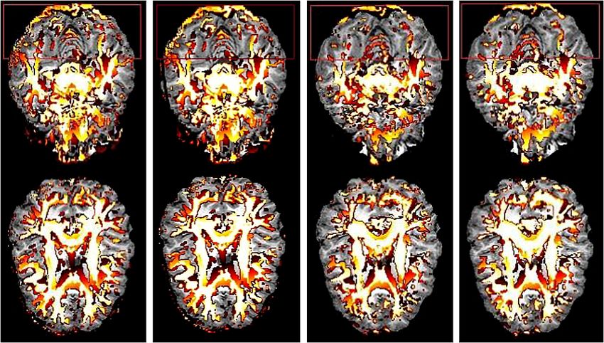
202                  YU, ZHANG, ALEXANDER AND DAVIDSON

                        F IG . 1.   Ellipsoid representation of a DT.

of D, respectively, correspond to the orientations and the lengths of axes in an
ellipsoid representation (see Figure 1). The distance between the center and any
point on the surface of the ellipsoid measures the rate of the water diffusion along
that particular orientation in the voxel.
   One of the main themes in DTI research is to identify the anisotropic water dif-
fusion brain areas, which facilitates the downstream fiber tracking process. There
are two general strategies aiming to address this problem. The first is to construct
scalar measurements. The anisotropic water diffusion areas are then identified
based on thresholding these scalar measurements. Reviews of this type of method
can be found in Moseley et al. (1990), Douek et al. (1991), van Gelderen et al.
(1994), Basser and Pierpaoli (1996), Johansen-Berg and Behrens (2009), among
others. Thresholding the fractional anisotropy (FA) and the relative anisotropy
(RA) [see Section 2.3; Basser and Pierpaoli (1996)] has gained popularity and
has been widely adopted by neuroscientists in the past decade. Nonetheless, FA
and RA are essentially defined as functions of the eigenvalues of the DT estimate
in every brain voxel. These eigenvalues typically carry systematic bias [see Sec-
tion 3; Pierpaoli and Basser (1996), Zhu et al. (2007), Jones (2003), Lazar and
Alexander (2003)], the magnitudes of which are sensitive to the distribution of
the noise carried in raw DWI data, and therefore significantly affect the effective-
ness and validity of FA (RA) based methods in practice. The second is to classify
the morphologies of DTs via test-based approaches [Zhu et al. (2006), Zhu et al.
(2007)], which not only quantify the degree of water diffusivity in each voxel,
but also lend theoretical supports to statistical inference. However, to the best of
our knowledge, all existing approaches on this respect are single-voxel based. The
validity and performance of these methods rely essentially on the technical re-
quirement that the number of diffusion gradients in the DWI experiment is large
and ultimately diverging to infinity. Moreover, the DTI data are typically spatially
structured. Ignoring the spatial information may diminish the effectiveness of the
methods.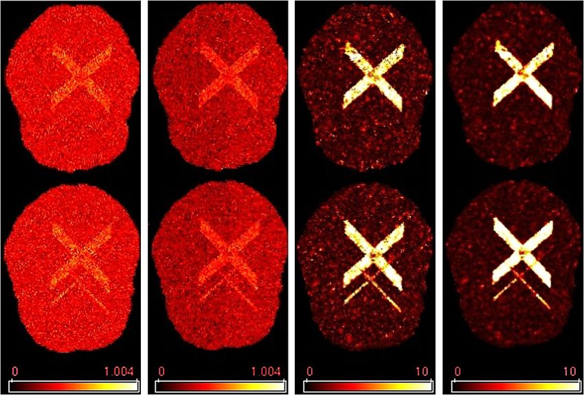
LOCAL TESTS FOR ANISOTROPIC AREAS                          203

   In this paper, we develop new test-based approaches to identify the anisotropic
water diffusion brain areas, which are usually associated with areas passed by fiber
tracts. To this end, for each voxel, we examine the testing problem “all three eigen-
values are equivalent” against “at least two eigenvalues are different.” The former
corresponds to isotropically diffused DTs, whereas the latter includes anisotropi-
cally diffused DTs with morphologies of prolate, oblate and nondegenerate. Our
proposed test statistic accommodates the spatial information of the imaging space
by taking into account eigenvalues in neighboring voxels. Under mild regularity
conditions, we demonstrate that our proposed test statistic asymptotically follows
a χ 2 distribution. Therefore, the performance of our methods in the identification
of fiber areas is not affected by the bias components carried in the eigenvalue es-
timates. In theory, one of the main technical requirements is the divergence of the
number of neighboring voxels involved in the construction of the statistic. This
differs from the divergence of the number of diffusion gradients typically assumed
by test-based approaches. Therefore, our methods shed light on alternative ways of
improving the identification accuracy of anisotropic water diffusion areas. Further-
more, an adaptive procedure to select varied neighborhoods is proposed to solidify
the performance of our proposed approaches when the acquired imaging data have
limited resolution. Simulation studies and real data examples are provided to illus-
trate the efficacy of our proposed methods.
   The rest of the paper is organized as follows. Section 2 introduces the back-
ground related to our study. Section 3 establishes a statistical model based on
eigenvalues in the selected neighborhood of a single voxel. Section 4 describes the
procedure of constructing our proposed test statistic, and an adaptive method for
selecting neighboring voxels. Section 5 explores the theoretical properties of our
proposed test statistic. Section 6 presents simulation results. There, our methods
are compared with FA-threshold and Smooth-FA-threshold approaches. Section 7
applies all approaches on real brain DTI data. Section 8 discusses our findings in
this paper. Technical conditions and proofs are given in a supplemental document.

  2. Background. We begin with a brief introduction of DWI data, DTI data
and existing statistical models for estimating DTI data from DWI data. Then, we
summarize the associations among fiber tracts, tissue types, water diffusivity and
DT types. After that, we overview the quantitative scalars, FA and RA, popularly
used in fiber tracking algorithms.

   2.1. From DWI to DTI. In this section we first give a brief introduction of the
structures of DWI and DTI data, where the former are acquired from the diffusion
weighted magnetic resonance experiment, while the latter are estimated from the
former based on some statistical model. Then, we summarize the existing statisti-
cal models for estimating DTI data from DWI data.
   We assume that the DWI data over the brain of a given subject contain N
voxels, each of which consists of diffusion-weighted measurements. Denote by
204                  YU, ZHANG, ALEXANDER AND DAVIDSON

φ0 , b, {(φi , gi )}ri=1 , the acquired diffusion-weighted measurements at a given
voxel over the brain in a DWI experiment. Here, the ith diffusion gradient gi =
(gi,1 , gi,2 , gi,3 )T , with gTi gi = 1, is chosen by the experimenter before the DWI
experiment starts, and serves as a scanning direction in the experiment [Hasan,
Parker and Alexander (2001)]; b is the b-factor, whose value is determined by a
function of parameter settings in the DWI experiment [Stejskal and Tanner (1965),
Moseley et al. (1990), Anderson (2001)]; both gi and b usually adopt the same
values over all voxels in a DWI experiment; φi denotes the diffusion attenuated
signal, acquired on the ith diffusion gradient gi at b; φ0 is the reference signal
obtained at b = 0; {φi }ri=1 and φ0 compose the responses of the DWI experiment
for each voxel; r is the number of acquired attenuated signals for each voxel.
   Accordingly, a single-voxel of the DTI data contains a 3 × 3 symmetric, positive
definite DT matrix,
                                ⎡
                                 D1,1     D1,2   D1,3 ⎤
                           D = ⎣ D1,2     D2,2   D2,3 ⎦ ,
                                 D1,3     D2,3   D3,3
which carries the intrinsic information of water diffusion in that particular voxel.
The elements of D can be reorganized as a 6 × 1 vector d = (D1,1 , D2,2 , D3,3 ,
D1,2 , D1,3 , D2,3 )T .
   The connections between DWI and DTI data are first investigated by the seminal
work of Basser, Mattiello and LeBihan (1994), in which the following multivariate
linear and nonlinear regression models are proposed. For a single-voxel,
(2.1)      multivariate linear model:    log(φi ) = log(φ0 ) − bxTi d + εi ,

(2.2)      multivariate nonlinear model:     φi = φ0 exp −bxTi d + ηi ,
where i = 1, . . . , r, xi = (gi,1
                               2 , g 2 , g 2 , 2g g , 2g g , 2g g )T , ε and η
                                    i,2 i,3      i,1 i,2 i,1 i,3 i,2 i,3    i      i
are random errors. d is then estimated from either model by regression techniques.
   A number of alternative statistical models as well as fitting procedures, besides
Basser, Mattiello and LeBihan (1994), have been proposed to obtain sophisticated
DT estimates from DWI data concerning various aspects, such as robustness, bias,
non-Gaussian errors, spatial smoothness, model validity, etc. Examples include
Mangin et al. (2002), Chang, Jones and Pierpaoli (2005), Salvador et al. (2005),
Heim et al. (2007), Zhu et al. (2007), Tabelow et al. (2008) and many others.

   2.2. Fiber tracts, tissue types, water diffusivity and DT types. The associations
among fiber tracts, tissue types, water diffusivity and DT types are summarized as
follows. For voxels located in fiber tracts, that is, white matter brain areas, water
tends to present higher diffusivity along the dominant orientation of fibers than
that in other orientations. DTs in these voxels are anisotropic, characterized by
the heterogeneity in lengths of axes in the corresponding ellipsoid representations.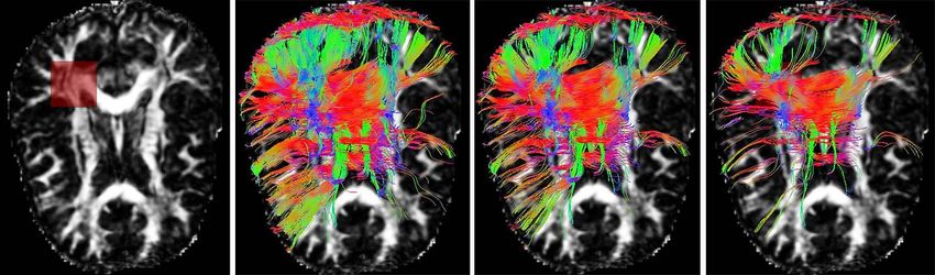
LOCAL TESTS FOR ANISOTROPIC AREAS                                       205

                        F IG . 2.   An illustrative example of fiber tracts.

In contrast, for voxels in brain areas without fiber tracts, that is, grey matter ar-
eas, DTs are isotropic. In these areas, the diffusivity of water in all orientations is
roughly the same. Therefore, the corresponding represented ellipsoids are spheri-
cally shaped. The morphology of an anisotropic DT can usually be classified into
one of the three categories, namely, prolate, oblate and nondegenerate, respec-
tively, corresponding to brain voxels located in uniquely orientated fiber tracts
(Area 1 in Figure 2), crossed fiber tracts with similar intensities on two or more
different orientations (Area 2 in Figure 2, characterized by similar fiber denseness
for the red and blue bundles in their intersected parts) and crossed fiber tracts with
distinct intensities on different orientations (Area 3 in Figure 2, characterized by
the scenario that the denseness of blue tracts is higher than that of green tracts in
their intersected parts).
   A vast number of tractography algorithms have been proposed in order to re-
construct fiber tracts in the human brain based on DTI data. A list of examples
of these algorithms can be found in Conturo et al. (1999), Gössl et al. (2002), Xu
et al. (2002), Behrens et al. (2007), O’Donnell and Westin (2007) and many others.
We observe that most of these approaches are founded on the derived voxel-wise
scalar quantities, such as FA and RA, which summarize/extract microstructural
information of water diffusion carried by DWI or DTI data.

   2.3. Quantitative scalars: FA and RA. The fractional anisotropy (FA) and rel-
ative anisotropy (RA) [Basser and Pierpaoli (1996)] are quantitative scalars widely
used by neuroscientists to measure the water diffusivity in brain tissues and con-
struct algorithms for tracking fibers, since they are computationally simple and
invariant in the choice of the laboratory coordinate system and diffusion gradients.
For a given voxel, FA and RA are defined as

                                                                        k=1 {λ(k) − λ(·) }
                                                                        3                 2
                      k=1 {λ(k) − λ(·) }
                      3                 2
                  3                                      3
       FA =                3    2
                                          ,         RA = √                  3
                                                                                            ,
                  2        k=1 λ(k)                       2                 k=1 λ(k)
206                       YU, ZHANG, ALEXANDER AND DAVIDSON

where λ(·) = {λ(1) + λ(2) + λ(3) }/3, with λ(3) ≥ λ(2) ≥ λ(1) being the ordered eigen-
values of the DT estimate.
   Under the ideal but unrealistic assumption that the estimated DT is noise
free, RA√ = 0 and FA = 0 in isotropic voxels [i.e., λ(1) = λ(2) = λ(3) ], whereas
RA = 3 and FA = 1 in purely anisotropic voxels [i.e., λ(3)  λ(2) = λ(1) ].
However, the noise carried by the DWI data contaminates the DT estimates, and
subsequently introduces systematic bias into the derived eigenvalues [Pierpaoli
and Basser (1996)]. Although these bias components have been investigated by
numerical evaluations [Jones (2003), Lazar and Alexander (2003)] as well as
in theory [Zhu et al. (2007)], the magnitudes are sensitive to the distribution
of the noise in DWI experiments. Consequently, these bias components intro-
duce uncertainty into the constructed FA and RA. In practice, brain areas with
small but nonvanishing FA (RA) usually correspond to grey matter areas, whereas
those with large FA (RA) are typically areas passed by fiber tracts. Some trac-
tography algorithms are based on FA or RA with thresholds (e.g., the trac-
tography algorithm integrated in MedINRIA, a publicly available software at
http://www-sop.inria.fr/asclepios/software/MedINRIA). The thresholds, however,
are usually manually chosen by investigators based on their historical knowledge
of the DTI data and the structure of the human brain.
   Figure 3 illustrates how the fiber tracking results are affected by distinct ex-
periential thresholds of the FA, where the detailed data information is given in
Section 7. We use a region of interest (ROI) with 30 × 30 voxels, which is high-
lighted by a red rectangle shown in the leftmost panel of Figure 3. The tracked
fibers passing through the ROI using distinct FA thresholding criteria, namely,
FA > c with c = 0.3, 0.45 and 0.6, are displayed in the remaining three panels of
Figure 3. All sub-figures in Figure 3 are constructed by MedINRIA, where differ-
ent colors stand for different principal orientations of the corresponding DTs. We
observe that the fiber tracking results are sensitive to the FA threshold, the choice
of which, owing to the uncertainty of the bias magnitudes in eigenvalue estimates,

F IG . 3. Fiber tracking results by distinct FA thresholds. From left to right: FA map with a ROI high-
lighted; constructed fibers passing through the ROI by FA thresholds 0.3, 0.45 and 0.6, respectively.
LOCAL TESTS FOR ANISOTROPIC AREAS                            207

is not well supported in theory. In other words, there is lack of a criterion to choose
the threshold for FA, and justify the goodness of the tracking results.
   A more sophisticated approach based on FA is due to Zhu et al. (2006), in
which the asymptotic distribution of a test statistic established on FA is investi-
gated. Therefore, it is capable of suggesting a threshold to be used. This approach,
however, is not applicable in our study, since the theory needs the assumption
that the number of gradients for every brain voxel is diverging to infinity, that is,
r → ∞. In contrast, in our study r = 12.
   Another limitation of FA and RA with threshold approaches is that the DTI data
are typically spatially structured. FA and RA, however, are defined as functions of
the eigenvalues of the DT in every single voxel. These approaches identify the ex-
istence of fibers in each voxel while ignoring the spatial information, and therefore
may diminish the effectiveness in the downstream fiber tracking algorithms.
   We observe that there exist approaches which accommodate the spatial infor-
mation in the stage of DT estimation, such as Heim et al. (2007) and Tabelow
et al. (2008). Intuitively, by incorporating the spatial information, these methods
improve the DT estimation, and therefore the accuracy of FA and RA. Hereafter,
we refer to the FA based on DT estimated by the approach in Tabelow et al. (2008)
and Polzehl and Tabelow (2009) (implement in R package dti) as Smooth-FA. In
our numerical studies, Smooth-FA with threshold, namely, Smooth-FA-threshold,
is employed as an approach to identify anisotropic brain voxels, and is compared
with our proposed methods.

    3. Statistical model on local eigenvalues. We consider the DTI data of a
given subject with N voxels. In each voxel v ∈ {1, . . . , N}, denote by D(v) (with-
out confusion, we concisely denote D) the DT estimated from a statistical model
in Section 2.1. Let λ(3) ≥ λ(2) ≥ λ(1) be the ordered eigenvalues of D. In practice,
these eigenvalues are adopted to estimate the ordered true eigenvalues, denoted by
λ∗(3) ≥ λ∗(2) ≥ λ∗(1) .
    It has been demonstrated both in numerical studies and in theory that E{λ(3) } >
λ(3) and E{λ(1) } < λ∗(1) . Such a bias is actually caused by the sorting procedure in
  ∗

the decomposition of D. In other words, we can postulate that one of the eigen-
values of D, that is, λk ∈ {λ(k) : k = 1, 2, 3}, is associated with λ∗(k) (but we don’t
know which one it is). Here, “associated” means there exists a random error εk
with E(εk ) = 0 such that
(3.1)                              λk = λ∗(k) + εk .
However, λ∗(k) is estimated by λ(k) instead of λk . Therefore, E{λ(3) } > E(λ3 ) =
λ∗(3) . Similar arguments lead to E{λ(1) } < λ∗(1) . The magnitudes of the bias compo-
nents are sensitive to the distribution of the noise in DWI experiments, introducing
uncertainty into the quantitative scalars, such as FA and RA.
    In our approach, instead of using the eigenvalues at a single voxel v only,
we choose a set of n neighboring voxels located adjacent to v. Denote by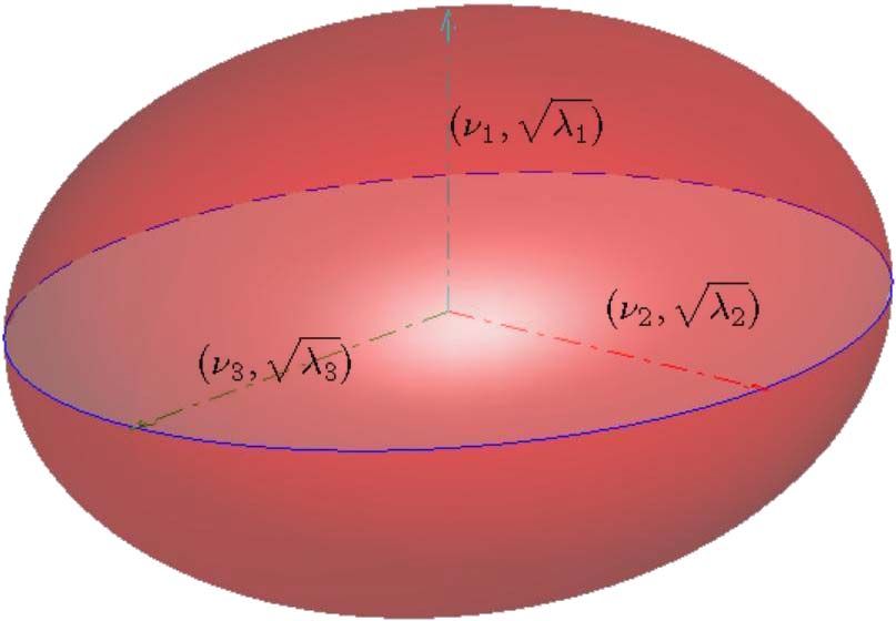
208                     YU, ZHANG, ALEXANDER AND DAVIDSON

{λj,(k) (v) : k = 1, 2, 3}nj=1 [i.e., λj,(k) ] the eigenvalue estimates in the selected
neighboring voxels, whose permuted version associated with the set of true eigen-
values is denoted by {λj,k (v) : k = 1, 2, 3}nj=1 (i.e., λj,k ). Here, j = 1 corresponds
to voxel v, that is, λ1,k = λk .
   Similar in spirit to the random complete block design, we model E(λj,k ), the
expected eigenvalue of the j th neighboring voxel of v, as the addition of two com-
ponents, namely, the true eigenvalue λ∗(k) for voxel v and the difference of eigen-
values between voxel v and its j th neighboring voxel, denoted by βj . That is,
E(λj,k ) = λ∗(k) + βj , which leads to the additive model,
(3.2)                            λj,k = λ∗(k) + βj + εj,k ,
where the eigenvalues {λ∗(k) : k = 1, 2, 3} in voxel v are of primary interest and
therefore treated as the treatment effects, whereas the differences of eigenvalues
between voxel v and its neighboring voxels {βj }nj=1 are the blocking effects and
serve as nuisance parameters; {εj,k : k = 1, 2, 3}nj=1 are random errors. Clearly,
β1 = 0, such that (3.2) complies with (3.1) when j = 1.
   Nonetheless, as discussed above, based on the DT estimates, we can only ob-
tain {λj,(k) , k = 1, 2, 3}, the ordered version of {λj,k , k = 1, 2, 3}. In other words,
the values of λj,k are not available in practice. Therefore, the well-developed tech-
niques for the additive model in a complete block design are not directly applicable
in analyzing model (3.2). We borrow its basic idea and integrate the corresponding
contrast test statistic as one of the main parts in our proposed test statistic. The
technical properties of our proposed test statistic in isotropically diffused DT vox-
els, that is, λ∗(3) = λ∗(2) = λ∗(1) , then rely on the fact that λj,(k) = λ∗(1) + βj + εj,(k) .

   4. Local test based on neighboring eigenvalues.

    4.1. Test of hypotheses. Classifying the tissue types for a particular brain
area plays a key role in the downstream fiber tracking algorithms. In voxels
without fibers, water tends to diffuse in an isotropic manner, characterized by
the eigenvalue property λ∗(3) ≈ λ∗(2) ≈ λ∗(1) . In contrast, water in voxels passed
by fiber tracts usually presents anisotropic diffusion. DTs in these voxels typi-
cally have three possible morphologies, namely, prolate λ∗(3) > λ∗(2) ≈ λ∗(1) , oblate
λ∗(3) ≈ λ∗(2) > λ∗(1) and nondegenerate λ∗(3) > λ∗(2) > λ∗(1) , respectively, correspond-
ing to brain voxels located in uniquely oriented fiber areas, crossed fiber areas with
roughly the same fiber intensities and crossed fiber areas with distinct fiber inten-
sities. In summary, anisotropy is characterized by either λ∗(3) > λ∗(2) or λ∗(2) > λ∗(1) .
Therefore, we consider the hypothesis testing problem,
(4.1)     H0 : λ∗(3) = λ∗(2) = λ∗(1)   vs.   H1 : λ∗(3) > λ∗(2)   or   λ∗(2) > λ∗(1)
for each voxel v. This testing problem can be reformulated as a form of contrast
test,
(4.2)   H0 : Aλ∗ = 0 vs.        H1 : A(l, ·)λ∗ > 0         for l = 1, or, . . . , or μ,
LOCAL TESTS FOR ANISOTROPIC AREAS 209
where λ∗ = (λ∗(3) , λ∗(2) , λ∗(1) )T , A is a full row rank matrix with rank(A) = μ and
l2 =1 A(l1 , l2 ) = 0 for l1 = 1, . . . , μ. There exists more than one possible choice
3
of A, such that hypothesis testing problems (4.1) and (4.2) are equivalent. For
example,
1 −1 0
(4.3) A= ,
0 1 −1
which is adopted in our numerical studies. Clearly, μ = 2.
To test (4.2), for each voxel v, we propose the test statistic K, represented by
(4.4) K = n(Un − −1 (Un −
θ Un )T θ Un ),
√
where Un = (Aλ· / MSE) · S·2 ; λ· = (λ·,(3) , λ·,(2) , λ·,(1) )T ; λ·,(k) = n
j =1 λj,(k) /
n, k = 1, 2, 3; S·2 is the mean of Sj2 over the neighboring voxels of v; Sj2 =
k=1 {λj,(k) − λj,(·) } /2, j = 1, . . . , n; MSE = j =1 k=1 {λj,(k) − λ·,(k) −
3 2 n 3
0 be an estimate of V0 , the set of isotropic voxels
λj,(·) + λ·,(·) }2 /{2(n − 1)}; let V
over the entire brain; θ Un denotes the sample median of Un over V 0 ;
denotes the
√
sample covariance of nUn over V0 . V0 is obtained from the following iteration
steps:
(i) Evaluate Un ’s over all voxels of interest. For some pre-given significant
2
level α, let χμ;1−α be the (1 − α)th quantile of the chi-square distribution with μ
degrees of freedom.
0,0 include all voxels of interest.
(ii) Let V
denote the statistic computed
(iii) In the sth iteration (s = 1, 2, . . .), let K
from (4.4) based on V 0,s−1 , and let K = cK.
(iv) Include voxel v in V0,s if the corresponding statistic K < χμ;1−α
2 .
(v) Repeat steps (iii) and (iv) until θ Un converges.
In step (iii) above, the constant c is to correct the bias in the evaluation of K.
This is because in the sth iteration,
θ Un in K is constructed by only using voxels in
V0,s−1 , which includes voxels with K capped by χμ,1−α2 in the (s − 1)th iteration.
The value of c is derived as follows:
1
cK
E KI < χ2
μ;1−α ≈ n(Un − −1 (Un −
θ Un )T θ Un )
|V0,s−1 |
v:cK210 YU, ZHANG, ALEXANDER AND DAVIDSON
is the sample covariance of
where “=” is followed by the fact that in step (iii),
√
nUn over V0,s−1 ; I(·) is the indicator function. Therefore,
E KI K < χμ;1−α cK
= E cKI < χ2
μ;1−α ≈ cμ.
2
(4.5)
On the other hand, according to Theorem 1 in Section 5, K is approximately χμ2
distributed,
χ2
t μ/2
e−t/2 dt.
μ;1−α
(4.6) E KI K < χμ;1−α
2
≈
0 2μ/2 (μ/2)
1 χμ;1−α
2
t μ/2
Combining (4.5) and (4.6), we set c = μ 0 2μ/2 (μ/2)
e−t/2 dt.
R EMARK 1. We now make some remarks concerning the construction of the
statistic in (4.4). The main term Un in K consists of two parts:
√
• The first part Aλ· / MSE mimics the t statistic of the contrast test for the
additive model in a complete block design. Referring to the proofs of Theo-
rems 1 and 2, under certain regularity conditions, it approaches infinity with rate
√
n, when there are significant differences among {λ∗(k) : k = 1, 2, 3}, whereas it
converges to a fixed constant when λ∗(3) = λ∗(2) = λ∗(1) . Therefore, it has good
statistical power in identifying the differences among {λ∗(k) : k = 1, 2, 3}, when
model (3.2) is valid.
• The second part S·2 is added to increase the power of the test statistic K on
the boundary of fibers. For any voxel on the boundary of fibers, in the sense that
its selected neighborhood contains voxels belonging to both fiber and nonfiber
areas, the assumption that the collected eigenvalues in the selected√neighboring
voxels follow model (3.2) may not be appropriate. In this case, MSE √ tends
to inflate and, consequently, the statistical power of the √
first part Aλ· / MSE is
limited. The second part then counteracts the effect of MSE, and therefore is
particularly useful when the resolution of the DTI data is limited.
• Furthermore, θ Un , the sample median instead of sample mean of Un , is adopted
just to ensure the robustness of the approach.
R EMARK 2. In this paper we establish testing procedures for identifying the
brain areas with fiber tracts. However, for voxels located in fiber tracts, their DTs
have three possible morphologies, namely, prolate, oblate, and nondegenerate, re-
spectively, corresponding to eigenvalue properties λ∗(3) > λ∗(2) ≈ λ∗(1) , λ∗(3) ≈ λ∗(2) >
λ∗(1) , and λ∗(3) > λ∗(2) > λ∗(1) . One may also implement similar testing procedures as
those in this paper to further classify these three possibilities. We leave the details
out for presentational brevity.LOCAL TESTS FOR ANISOTROPIC AREAS 211
4.2. Adaptive selection of neighborhood. Following Sections 4.1 and 5, the
asymptotic theories for K need that the neighborhood size n is large and that
model (3.2) is satisfied. From the experimental point of view, as long as the reso-
lution in a DWI experiment is sufficiently good, such that the proportion of vox-
els located on the boundary of fibers over the entire brain shrinks, we can sim-
ply employ a fix-shaped neighborhood in the construction of K (e.g., choose the
neighborhood as a fixed cube). However, for experiments with limited resolution,
a fix-shaped neighborhood may not be a good choice, because in this case, the
assumption that the eigenvalues in the neighboring voxels follow model (3.2) may
not be well satisfied, in order to ensure n large required by Theorem 1. Such a
problem is particularly severe for voxels located on the boundary of fibers. There-
fore, development of a varied neighborhood is necessary.
We propose an adaptive method to select the neighboring voxels based on the
philosophy below. First, the adjacent voxels of v should have a better chance to
be selected as neighboring voxels than those far away. Second, to ensure the va-
lidity of model (3.2), if the tensor in v is isotropic, the selected neighborhood
should mainly consist of voxels with isotropic tensors. Likewise, if the tensor
in v is anisotropic, the selected neighborhood should be in favor of voxels with
anisotropic tensors. Therefore, we incorporate the physical distances and similar-
ity measures of DTs between voxel v and its nearby neighbors to establish the
criteria for selecting neighboring voxels.
For each voxel v and fixed number n of neighboring voxels, we summarize our
proposed adaptive neighborhood selection approach as follows:
(1) Fix a cube-shaped domain centered at v with reasonably large size x ×y ×z,
whose voxels are candidates. Here x, y, z are integers and xyz ≥ n.
(2) Define the similarity score function f between voxel v and its neighboring
candidate vl , l = 1, . . . , xyz, as
f (v, vl ) = dD D(v), D(vl ) exp C · dp (v, vl ) ,
where dp (v, vl ) denotes the physical distance between voxels v and vl ; dD (D(v),
D(vl )) = trace[{D(v) − D(vl )}2 ] is a measurement of the diffusion similarity be-
tween tensors in voxels v and vl [Alexander, Gee and Bajcsy (1999)]; C ≥ 0 is
added to balance the contribution of dp (v, vl ) and dD (D(v), D(vl )).
(3) Select n voxels with the lowest f values as the neighboring voxels.
We observe that C in f is adopted to balance the contribution of dD (D(v),
D(vl )) and dp (v, vl ). When the resolution of the DTI data is high, dp (v, vl ) is close
to 0. Consequently, for any fixed C, exp{C · dp (v, vl )} approaches the constant 1.
Therefore, for high resolution DTI data, the proposed approach is not sensitive to
the choice of C. Throughout our numerical studies, we fix C = 0.1.
We would like to point out that the proposed approach above is similar in spirit
to the adaptive approaches in Tabelow et al. (2008) and Li et al. (2011), where it-
erative testing procedures are used to adaptively control the contribution of neigh-
boring voxels in their proposed algorithms. Compared with their approaches, our212 YU, ZHANG, ALEXANDER AND DAVIDSON
approach is computationally more economic. The effectiveness of our proposed
approach above has been demonstrated in Yu (2009) by simulation studies.
We summarize our proposed procedure of constructing K in the supplemental
document [Yu et al. (2013)].
5. Theoretical properties. In this section we explore the theoretical proper-
ties of our proposed test statistic K. The technical details are given in the supple-
mental document [Yu et al. (2013)]. Theorem 1 below establishes the asymptotic
null distribution of K, when the number n of neighboring voxels is large.
T HEOREM 1. Assume model (3.2) and Condition A in the supplemental doc-
ument. Then for K defined in (4.4), under the null hypothesis in (4.2), as n → ∞,
L
K → χμ2 .
We would like to point out that the construction of K and the theoretical
derivations of Theorem 1 are nontrivial and challenging. Following the discussion
in Section 3, for each voxel v, we postulate that there exist unobservable one-
to-one correspondences, that is, {(λk , λ∗(k) ) : k = 1, 2, 3}, between the estimated
and true eigenvalues. The ordered eigenvalue estimates λ(3) ≥ λ(2) ≥ λ(1) , how-
ever, are neither unbiased estimates for λ∗(3) ≥ λ∗(2) ≥ λ∗(1) , nor independent. We
address these bias components in the construction of K and the corresponding
proof of Theorem 1 based on the intuition as follows. Referring to model (3.2),
for an isotropic voxel v, the collected neighboring voxels can be modeled as
λj,(k) = λ∗(1) + βj + εj,(k) . As such, the bias components of eigenvalue estimates
in the neighboring voxels of v are carried by εj,(k) , whose effects in our test statis-
tic are counteracted by θ Un constructed based on spatial information of the entire
brain.
To appreciate the discriminating power of K in the identification of anisotropic
brain areas, the asymptotic power of K is established in Theorem 2 below.
T HEOREM 2. Assume model (3.2) and Condition A in the supplemental doc-
ument. Then for voxel v, under the fixed alternative H1 in (4.2), as n → ∞,
P
n−1 K → M,
where M is given by (A.4.3) in the supplemental document.
P
Theorem 2 shows that as long as g( a(v)) = g(b), M > 0 and K → +∞ at
rate n, under the fixed alternative H1 . Here, g(·) is defined by (A.3.2) in the supple-
mental document; a(v) = (E{2S12 (v)}, E{λ1,(3) (v)}, E{λ1,(2) (v)}, E{λ1,(1) (v)})T ;
b = (E(2Sε2 ), E{ε1,(3) (1)}, E{ε1,(2) (1)}, E{ε1,(1) (1)})T ; S12 (v) and Sε2 are, respec-
tively, the sample variances of {λ1,(k) (v), k = 1, 2, 3} and {ε1,(k) (1), k = 1, 2, 3}.LOCAL TESTS FOR ANISOTROPIC AREAS 213
Thus, under the fixed alternative, the power of our proposed test statistic K tends
to 1 except in rare situations. Corollary 1 below gives one specific example of
M > 0. The proof is straightforward and omitted.
C OROLLARY 1. Assume conditions in Theorem 2. Suppose that εj,k has a
symmetric distribution about 0, that is, εj,k has the same distribution as −εj,k ,
and E{λ1,(3) } − E{λ1,(2) } = E{λ1,(2) } − E{λ1,(1) }. Then M > 0.
6. Simulation study.
6.1. Basic settings for numerical work. Since in a real DTI data set, the num-
ber of voxels, each of which corresponds to a hypothesis test, is typically large,
false discovery rate (FDR) techniques [Benjamini and Hochberg (1995), Storey
(2002), Storey, Taylor and Siegmund (2004), Zhang, Fan and Yu (2011)] are in-
corporated in our numerical works to control the error rates. Two FDR procedures
are employed in our study, namely, the conventional FDR procedure by Storey
(2002) and the FDRL procedure by Zhang, Fan and Yu (2011), which is capable of
capturing the spatial information in imaging data. A short summary of the FDRL
procedure is provided in the supplemental document [Yu et al. (2013)].
Some settings of parameters throughout our numerical works are given as fol-
lows. For FDR and FDRL procedures, set false discovery control level as 0.01
and tuning parameter λ = 0.2. The neighborhood for the FDRL procedure is set
as the nearest 7 voxels shown in the left panel of Figure 4. When evaluating K
for each voxel, A is given by (4.3). Apply the adaptive neighborhood selection ap-
proach proposed in Section 4.2 to select neighboring voxels, where the domain for
F IG . 4. Left panel—neighbors of a voxel used in the FDRL procedure. Right panel—gometry of
the simulated brain.214 YU, ZHANG, ALEXANDER AND DAVIDSON
the candidate neighboring voxels is set as a 5 × 5 × 3 cube centered at v. There,
n = 25 voxels are selected based upon f with C = 0.1. The choice of n is referred
to in the results in Section 6.3: when n = 25, the sampling distribution of K agrees
reasonably well with the χ 2 distribution.
6.2. Data simulation. We simulate several sets of DWI data over the entire
brain. For each set, a 3D imaging space with the same brain areas as the real
DWI data in Section 7 is simulated, where fiber tracts are simulated to have the
geometrical structure displayed in the right panel of Figure 4. DTs are simulated
according to the locations of voxels in the imaging space. To this end, four dis-
tinct sets of eigenvalues, namely, [0.7, 0.7, 0.7], [1.0, 0.55, 0.55], [0.8, 0.8, 0.5]
and [0.9, 0.7, 0.5] (units: 10−3 mm2 /s), are adopted to, respectively, simulate DTs
with morphologies of isotropic (nonfiber areas), prolate (single blue and red bun-
dles), oblate (intersected areas of blue bundles) and nondegenerate (intersected
areas between blue and red bundles), such that all simulated DTs share the same
mean diffusivity λ̄∗(·) = 0.7 × 10⁻³ mm2 /s, a typical value in real human brains
[Pierpaoli et al. (1996), Anderson (2001)].
Since the acquired attenuated signal intensity, φi (v), at each voxel v and gra-
dient gi in real DWI data is typically generated by the square-root of the sum
of squares of two random numbers in the DWI experiment [Henkelman (1985),
Salvador et al. (2005), Zhu et al. (2007)], we simulate a reference signal (i = 0)
and r = 12 diffusion attenuated signals (i = 1, . . . , 12) in each v [= (vx , vy , vz )]
as
2
φi (v) = φ0∗ (v) exp −bgTi D∗ (v)gi + εi,x (v) + εi,y
2 (v),
where φ0∗ (v) = 1200 when vx ∈ (0, 128], φ0∗ (v) = 1800 when vx ∈ (128, 256];
the b factor b = 1000 when i > 0, b = 0 when i = 0; diffusion gradients
{gi : i = 1, . . . , 12} are adopted from the real DWI data in Section 7; D∗ (v) =
Q(v) ∗ (v)QT (v); ∗ (v) = diag(λ∗(3) (v), λ∗(2) (v), λ∗(1) (v)); Q(v) is a 3 × 3 or-
thogonal matrix whose column vectors are composed of the eigenvectors of the
simulated D∗ (v),
⎡ √ √ ⎤ ⎡ √ √ ⎤
1/ √2 1/√2 0 1/√2 −1/√ 2 0
Q(v) = ⎣ −1/ 2 1/ 2 0 ⎦ or Q(v) = ⎣ 1/ 2 1/ 2 0 ⎦ .
0 0 1 0 0 1
Clearly, the former corresponds to the red and the corresponding parallel narrow
blue bundles in the right panel of Figure 4, while the latter models the other two
blue bundles. The random errors εi,x (v) and εi,y (v) are simulated as independent
and normally distributed with variance σ 2 , which is varied to provide signal to
noise ratios (SNRs), where SNR = φ0∗ (v)/σ . We examine four distinct SNRs, {5,
10, 15, 20}, each corresponding to one set of the simulated DWI data.LOCAL TESTS FOR ANISOTROPIC AREAS 215 F IG . 5. Empirical percentiles of K (y-axis) versus percentiles of χμ2 distribution (x-axis). Top panels—candidate cubic 5 × 5 × 3, n = 25. Bottom panels—candidate cubic 11 × 11 × 3, n = 81. From left to right panels: SNR = 10, 15 and 20. Solid line—the 45 degree reference line. 6.3. Agreement between χ 2 distribution and K. With the DWI data sets sim- ulated in Section 6.2, we estimate the DT in each voxel by regression model (2.1) and the corresponding eigenvalues by Schur decomposition. For each DWI data set, two sets (I and II) of K are constructed according to different settings of the adaptive neighborhood selection approach in Section 4.2. In particular, for Set I, the size of the candidate neighborhood and the number of selected neighboring voxels are, respectively, chosen as 5 × 5 × 3 and n = 25, while those for Set II as 11 × 11 × 3 and n = 81. Other settings are given in Section 6.1. For each simulated data set, we collect all K’s whose corresponding voxels are located inside the simulated nonfiber areas. The QQ plots of the (1st to 99th) percentiles of these K’s against those of the χμ2 distribution are displayed in Fig- ure 5, with top panels based on Set I, bottom panels on Set II. The left, middle and right panels correspond to SNR = 10, 15 and 20, respectively. Results in Figure 5 demonstrate that the sampling distributions of K, under both n = 25 and n = 81, agree reasonably well with the χ 2 distribution. 6.4. Receiver operating characteristic curve. We compare our methods (K- FDR and K-FDRL ) with FA with threshold (i.e., FA-threshold) and Smooth-FA with threshold (i.e. Smooth-FA-threshold) approaches by the receiver operating characteristic (ROC) curve, a widely adopted statistical tool for evaluating the ac- curacy of continuous diagnostic tests [Pepe (2003)].
216                    YU, ZHANG, ALEXANDER AND DAVIDSON

   Let {T1 , . . . , TN } be the set of statistics for all voxels over the entire brain, where
Tv for any voxel v ∈ {1, . . . , N} is the FA or Smooth-FA value, if the FA-threshold
or Smooth-FA-threshold approach is used; is the p-value based on K, if the K-
FDR approach is used; is the p        -value if the K-FDRL approach is used, where p
stands for the median smoothed p-value of K [Zhang, Fan and Yu (2011)]. For
any given threshold t, if we classify a voxel v as anisotropic based on Tv ∈ R(t),
where R(t) = {Tv : Tv ≥ t, v = 1, . . . , N} when Tv is the FA or Smooth-FA value;
R(t) = {Tv : Tv ≤ t, v = 1, . . . , N} when Tv is the p- or p      -value, then,

                                            v=1 I {Tv   ∈ R(t), H1 is true}
                                            N
                sensitivity:    se(t) ≡                                     ,
                                                         |V0 |

                                            v=1 I {Tv  ∈
                                            N
                                                       / R(t), H0 is true}
                specificity:    sp(t) ≡                                    ,
                                                      N − |V 0 |
where |V0 | is the number of isotropic voxels over the entire brain. The ROC curve
is then constructed as the 2D curve (se(t), 1 − sp(t)) when t ranges between 0
and 1. The area under the ROC curve (AUC) is a popularly adopted measure of
the accuracy of the test. More precisely, AUC is ranging between 0 and 1, and the
larger the AUC, the better the method.
   Following Sections 6.1 and 6.2, the ROC curves for FA, Smooth-FA, p and p
are displayed in Figure 6 for data sets with SNR = 5, 10, 15 and 20, respectively.
It has been seen from Figure 6 that the ROC curves of p    (dotted blue lines) and p
(dashed black lines) are consistently located above those of FA (solid red lines)
and Smooth-FA (dash-dotted green lines) for all simulated data sets, indicating
that K-FDR and K-FDRL are capable of achieving better classification accuracy
than FA-threshold and Smooth-FA-threshold approaches. Furthermore, the AUCs
of p in all examined data sets are superior to those of p, suggesting that K-FDRL
performs the best among all four approaches.

   6.5. Test results. In this section we present our test results in simulated data
sets. Settings of our computations are given in Section 6.1. For the sake of clarity,
we only present the results of SNR = 10. Those of SNR = 5, 15 and 20 display
similar phenomenon and are omitted.
   The FA threshold (>0.3003) and Smooth-FA threshold (>0.2803) are tenta-
tively chosen such that their identified results share the same sensitivity as K-
FDRL . The results of sensitivity and specificity by all four methods are displayed
in Table 1. Clearly, K-FDRL maximizes both the sensitivity (0.8845) and the
specificity (0.9982) in this example. K-FDR achieves similar specificity (0.9957)
but slightly smaller sensitivity (0.7522) compared to K-FDRL . However, in order
to yield comparable sensitivity (0.8845) as K-FDRL , FA-threshold and Smooth-
FA-threshold approaches produce much lower specificities (0.4012 for FA; 0.6242
for Smooth-FA).
LOCAL TESTS FOR ANISOTROPIC AREAS 217
F IG . 6. ROC curves for SNR = 5, 10, 15 and 20. Dashed black line—p-value of K; dotted blue
line—p -value of K; solid red line—FA; dash-dotted green line—Smooth-FA.
The performances of the four methods are further compared on two selected
axial slices. Throughout our simulation and real data examples, we apply the same
registration transformations from the brain data to the T1 high-resolution image of
the subject’s brain. The two slices with the simulated brain anisotropic areas high-
lighted are given in the leftmost panel of Figure 8. Figure 7 displays the color maps
of the FA, Smooth-FA, − log(p) and − log(p ), with all − log(p) and − log(p) val-
ues greater than 10 set equal to 10 to improve the visualization. Figure 8 compares
the detected anisotropic areas by FA > 0.3003, Smooth-FA > 0.2803, K-FDR and
K-FDRL for SNR = 10.
TABLE 1
Sensitivity and specificity, SNR = 10, the FDR control level is 0.01
Sensitivity Specificity
FA > 0.3003 0.8849 0.4012
Smooth-FA > 0.2803 0.8852 0.6242
K-FDR 0.7522 0.9957
K-FDRL 0.8845 0.9982218 YU, ZHANG, ALEXANDER AND DAVIDSON
F IG . 7. Comparison of color maps for simulated data set. From left to right: FA; Smooth-FA;
) by K. SNR = 10.
− log(p) by K; − log(p
As clearly evidenced in Figures 7 and 8, K-FDR and K-FDRL not only provide
detected results with better accuracy than FA-threshold and Smooth-FA-threshold
approaches, but also yield better contrasts between the significant areas and the
nonsignificant ones. In contrast, the results from FA (>0.3003) and Smooth-FA
(>0.2803) not only fail to detect some truly significant voxels, but also present
tiny scattered faulty findings, which expect to contaminate the downstream fiber
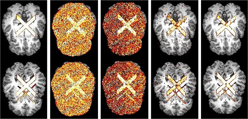
F IG . 8. Comparison of brain anisotropic areas discovered for the simulated data set. From left to
right: simulated brain anisotropic areas; FA > 0.3003; Smooth- FA > 0.2803; K-FDR; K-FDRL .
SNR = 10. The control level is 0.01.LOCAL TESTS FOR ANISOTROPIC AREAS 219
tracking results. It has been seen in the second to right and rightmost panels of
Figures 7 and 8 that the detected results by K-FDR and K-FDRL well capture the
primary features of the simulated anisotropic areas. Compared with K-FDR, the
K-FDRL approach offers slightly more accurate identifications in both isotropic
and anisotropic water diffusion areas.
7. Real data example. We apply our proposed testing procedures on five sub-
jects, whose DWIs were acquired by the magnetic resonance (MR) experiments
described below.
The brain magnetic resonance images (MRIs, including DWI and fMRI) of each
subject were acquired with a GE SIGNA 3-T scanner equipped with high-speed
gradients and a whole-head transmit-receive quadrature birdcage headcoil (GE
Medical Systems). The anatomical scan for each subject took approximately 20
minutes [Dalton et al. (2005)]. In the anatomical scanning, the size of each voxel
in an xy-plane is 0.9375 mm × 0.9375 mm, field of view = 24 cm2 , matrix =
256 × 256; 30 axial slices are acquired along the z-axis, slice thickness = 3 mm.
A single reference image at b = 0 and 12 diffusion-attenuated images with non-
collinear directions of diffusion gradients at b = 1000 s/mm2 were obtained. Since
we focus on the analysis of the anatomical structures of the human brain in this pa-
per, the detailed information for the functional scans is omitted.
Using the DWI data of a single subject as the representative, we first present and
compare the results by all four methods on two selected axial slices of the brain.
The results for the other four subjects display similar scenarios and are omitted.
The acquired data set contains 256 × 256 × 30 = 1,966,080 voxels with 400,309
voxels located inside the brain. In each voxel, the DT is estimated from regression
model (2.1). After that, the corresponding eigenvalues are obtained by Schur de-
composition.
All settings are given in Section 6.1. The color maps of FA, Smooth-FA,
− log(p) and − log(p ) are displayed in Figure 9 on two selected axial slices,
whereas the corresponding detected anisotropic diffusion brain areas by all four
methods are provided in Figure 10. As evidenced in Figure 10, compared with
the identified anisotropic areas by K-FDR or K-FDRL , FA-threshold and Smooth-
FA-threshold approaches produce more noisy detections. For example, inspection
of areas highlighted by red rectangles in the top panels of Figure 10 (enlarged in
Figure 11), FA > 0.35 and Smooth-FA > 0.35 detect more scattered tiny areas
than K-FDR and K-FDRL . Those are highly likely to be faulty findings. Further-
more, an overview of the areas located close to the top of the highlighted areas, FA
> 0.35 and Smooth-FA > 0.35 present more findings than K-FDR and K-FDRL .
However, those areas are located close to the boundary of the brain, and are most
likely to be nonfiber areas. In the meantime, as illustrated in Section 2.3, since
the number of gradients r in each voxel is small, FA-threshold and Smooth-FA-
threshold approaches cannot clearly infer and control the error rate of the iden-
tification, and therefore lack the rigorous criterion in selecting the appropriate220 YU, ZHANG, ALEXANDER AND DAVIDSON
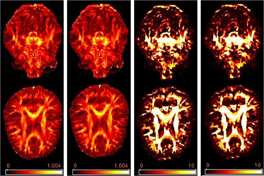
F IG . 9. Comparison of color maps for the real brain data set. From left to right: FA; Smooth-FA;
) by K.
− log(p) by K; − log(p
thresholds in practice. The superiority of our proposed methods to FA-threshold
and Smooth-FA-threshold approaches can be further illustrated by Figure 9, the
color maps of FA, Smooth-FA, − log(p) and − log(p ). The color maps of both
− log(p) and − log(p ) show better contrasts between the anisotropic and isotropic
areas than those of FA and Smooth-FA, indicating that K-FDR and K-FDRL more
effectively separate anisotropic diffusion areas from isotropic ones.
To further illustrate the efficacy of our methods in reducing the scattered
faulty findings, we summarize the frequency of identified isolated anisotropic
F IG . 10. Comparison of brain anisotropic areas discovered for the real brain data set. From left to
right: FA > 0.35; Smooth- FA > 0.35; − log(p) by K; − log(p) by K. The control level is 0.01.LOCAL TESTS FOR ANISOTROPIC AREAS 221
F IG . 11. Enlarged areas in the rectangles of Figure 10. Rotated 90◦ .
voxels over each subject’s brain for all four methods in Table 2. In particu-
lar, denote by N (v) = {v = (vx , vy , vz ) : |vi − vi | ≤ 1, for all i = x, y, and z}
the nearest neighboring voxels of v. Table 2 displays the number of vox-
els carried in S1,m (left) and S2,m (right) over each subject’s brain. Here
Su,m = {v : method m identify u voxels in N (v) as anisotropic}. Clearly, S1,m
carries voxels where only the voxel v itself is identified by method m over voxels
in N (v). Likewise, S2,m contains voxels where only two voxels, that is, the voxel
v itself and another voxel, are identified by method m over voxels in N (v). We
observe that voxels in S1,m and S2,m are highly likely to be faulty findings by
method m, since they are “isolated” from other identified anisotropic voxels; fiber
tracts, in contrast, are typically spatially connected.
It has been seen from Table 2 that our methods continue to outperform FA-
threshold and Smooth-FA-threshold approaches by producing much less isolated
findings. Compared with K-FDR, K-FDRL produces even a smaller number of
isolated identifications. Such a result is not surprising considering what has been
observed in Figures 7–10. Combining all the numerical results above, we therefore
recommend the identifications by K-FDRL as the final results.
8. Discussion. In DTI studies, one of the important research topics is to re-
fine the identification of the anisotropic water diffusion areas of human brain in
vivo. There are two general strategies aiming to address this problem. The first is
TABLE 2
Number of voxels carried in S1,m (left) and S2,m (right) over each subject’s brain
Subject Subject
Methods 1 2 3 4 5 1 2 3 4 5
FA > 0.35 323 360 348 356 280 718 770 720 758 671
Smooth-FA > 0.35 279 288 327 298 227 775 793 657 721 660
K-FDR 155 177 166 173 189 315 409 357 403 355
K-FDRL 63 77 100 93 103 129 158 149 212 138222 YU, ZHANG, ALEXANDER AND DAVIDSON
to improve the DT estimation. A downstream procedure is then needed to identify
the anisotropic water diffusion areas. The second is to refine the construction of
the scalar measurements or establish more powerful test statistics for every brain
voxel. The identification is then based on thresholding the measurements or a cer-
tain testing procedure. We observe that the second provides more intrinsic insight
into the water diffusivity in each voxel, and therefore is more effective in allusion
to the identification of anisotropic water diffusion areas.
From an experimental point of view, there are two ways to improve the acqui-
sition schemes for the DWI data. One is to increase the number of diffusion gra-
dients for every brain voxel, the other is to improve the resolution of the imaging
space, that is, increase the number of brain voxels. To the best of our knowledge,
existing methods for constructing scalar measurements or test statistics are all sin-
gle voxel based. Therefore, the corresponding inferences improve only when the
number of diffusion gradients in each voxel increases, while ignoring the possible
improvement of the resolution of the imaging space. The methods proposed in this
paper fill this gap by incorporating the eigenvalues in the neighboring voxels in the
construction of the test statistic K.
In this study we have established the asymptotic distribution of our proposed
test statistic. One of the main assumptions required by our theoretical results is
that the number of neighboring voxels for constructing K is large. This assump-
tion can be well achieved when the resolution of the imaging data is high. As such,
the bias components carried in the eigenvalue estimates no longer play a key role
in the identification of anisotropic water diffusion brain areas. In both simulation
and real data analysis, we have observed that our proposed K-FDR and K-FDRL
approaches lead to different identification results from FA-threshold and Smooth-
FA-threshold approaches, popularly adopted in the DTI community. In particular,
the scattered findings by our methods are much less than those by FA-threshold
and Smooth-FA-threshold approaches, indicating that by incorporating neighbor-
ing information, our methods are capable of screening out those isolated voxels
which are highly likely to be faulty findings. Results based on simulated DWI
data demonstrate that our proposed test statistic K agrees reasonably well with
the χ 2 distribution when n = 25 (or larger), and our methods achieve better accu-
racy than FA-threshold and Smooth-FA-threshold approaches in the identification
of anisotropic brain voxels. Furthermore, the Smooth-FA-threshold approach is ca-
pable of partially solving the bias problem in the eigenvalue estimates [Polzehl and
Tabelow (2009)]. However, the performance of the approach heavily replies on the
estimation of the heteroscedastic variances over the entire brain. These variances,
in turn, are modeled by a linear model and estimated using the reference signals
φ0 (v). We observe based on simulation studies that when the reference signals
over the entire brain are not homogeneous or do not share comparable variances as
attenuated signals φi (v), the performance of the approach varies [see more simula-
tion results provided in the supplemental document: Yu et al. (2013)]. In contrast,
under all these cases, our proposed K-FDRL approach consistently offers descent
results. We therefore conclude that over all four methods, our proposed K-FDRLLOCAL TESTS FOR ANISOTROPIC AREAS 223
approach performs the best over all our simulation studies. Unlike the simulation
examples, we are unable to show the true anisotropic (fiber) areas of the human
brains in real DTI data.
We would like to point out that in DTI studies, identification of anisotropic
water diffusion areas is just one step of the full analysis. Downstream analysis,
such as fiber tracking, is usually needed to fully capture the physical structure of
the human brain.
In this paper we have focused on establishing testing procedures to distinguish
anisotropic DT voxels from isotropic ones based on second order DT models. Our
proposed methods have been compared with the FA-threshold and Smooth-FA-
threshold approaches. The results of this paper can serve as a benchmark in ana-
lyzing the anatomical structures of human brains based on DTI data. We observe
that the following topics are highly related to this paper, and may absorb the inter-
est of the community in future research:
• With the idea of incorporating spatial information, single-voxel-based ap-
proaches, including FA, can possibly be improved by appropriately accounting
for the information in the neighboring voxels. Furthermore, in this paper, K is
established on the DTs estimated from model (2.1). Similar approaches can be
constructed based on more sophisticated DT estimates from other approaches.
• A similar strategy as that in this paper can be adopted to establish testing proce-
dures for teasing apart the morphologies of anisotropic DTs. Furthermore, the
basic ideas can be further extended to establish testing procedures for identify-
ing the presence of signals for data with spatial structures, though we focus on
DTI data in this paper.
• Another popular topic in DTI research is to consider higher-order tensor models
[Grigis et al. (2011) and therein], which are powerful tools for investigating
the fiber structures when there are several fiber bundles in a single voxel. The
local test idea in this paper can be possibly extended to identify the number of
intersected fiber bundles based on those higher-order tensor models.
Acknowledgments. We thank the Editor, the Associate Editor and four refer-
ees for invaluable suggestions, which greatly improved the quality of this paper.
SUPPLEMENTARY MATERIAL
Supplement to “Local tests for identifying anisotropic diffusion areas in
human brain with DTI” (DOI: 10.1214/12-AOAS573SUPP; .pdf). This file pro-
vides proofs for Theorems 1 and 2, a short summary of FDRL procedure [Zhang,
Fan and Yu (2011)], steps for constructing K based on DWI data and some more
simulation results.
REFERENCES
A LEXANDER , D., G EE , J. and BAJCSY, R. (1999). Similarity measures for matching diffusion ten-
sor images. In Proceedings of the 10th British Machine Vision Conference, 13–16 September
1999, University of Nottingham 93–102.You can also read