Super-resolving Herschel imaging: a proof of concept using Deep Neural Networks

MNRAS 000, 1–12 (2021) Preprint 23 September 2021 Compiled using MNRAS LATEX style file v3.0

 Super-resolving Herschel imaging: a proof of concept using Deep Neural
 Networks
 Lynge Lauritsen1★ , Hugh Dickinson1 , Jane Bromley2 , Stephen Serjeant1 , Chen-Fatt Lim3,4 ,
 Zhen-Kai Gao4,5 , Wei-Hao Wang4
 1 School of Physical Sciences, Faculty of Science, Technology, Engineering & Mathematics, The Open University,
 Walton Hall, Kents Hill, Milton Keynes, MK7 6AA, United Kingdom
 2 School of Computing & Communications, Faculty of Science, Technology, Engineering & Mathematics, The Open University,
arXiv:2102.06222v3 [astro-ph.GA] 22 Sep 2021

 Walton Hall, Kents Hill, Milton Keynes, MK7 6AA, United Kingdom
 3 Graduate Institute of Astrophysics, National Taiwan University, Taipei 10617, Taiwan
 4 Academia Sinica Institute of Astronomy and Astrophysics (ASIAA), No. 1, Section 4, Roosevelt Road, Taipei 10617, Taiwan
 5 Graduate Institute of Astronomy, National Central University, Taoyuan 32001, Taiwan

 Accepted XXX. Received YYY; in original form ZZZ

 ABSTRACT
 Wide-field sub-millimetre surveys have driven many major advances in galaxy evolution in the past decade, but without
 extensive follow-up observations the coarse angular resolution of these surveys limits the science exploitation. This has driven
 the development of various analytical deconvolution methods. In the last half a decade Generative Adversarial Networks have
 been used to attempt deconvolutions on optical data. Here we present an autoencoder with a novel loss function to overcome
 this problem in the sub-millimeter wavelength range. This approach is successfully demonstrated on Herschel SPIRE 500 µm
 COSMOS data, with the super-resolving target being the JCMT SCUBA-2 450 µm observations of the same field. We reproduce
 the JCMT SCUBA-2 images with high fidelity using this autoencoder. This is quantified through the point source fluxes and
 positions, the completeness and the purity.
 Key words: software: data analysis – submillimetre: galaxies – methods: data analysis

 1 INTRODUCTION the James Clerk Maxwell Telescope (JCMT) SCUBA-2 450 µm data
 compared to the Herschel SPIRE instrument to probe sub-millimetre
 All astronomical imaging has an intrinsic angular resolution limit,
 (sub-mm) number counts with fluxes below 20 mJy where source
 whether due to seeing, diffraction, instrumental effects or (in the case
 confusion becomes problematic in Herschel SPIRE data (Oliver et al.
 of an interferometer) the longest available baselines. In single-dish
 2010; Valiante et al. 2016). Further, Geach et al. (2013) also resolved
 diffraction-limited imaging, there is formally no signal on Fourier
 a larger part of the Cosmic Infrared Background than that possible
 scales smaller than the diffraction limit. This is because Fraunhofer
 using Herschel SPIRE. There has therefore been a great deal of in-
 diffraction is mathematically equivalent1 to a Fourier transform, so
 terest in developing algorithms for recovering or estimating some of
 the large-scale boundary of the telescope aperture also implies there
 the missing Fourier data on smaller angular scales (see Starck et al.
 is no image information smaller than some angular scale. For in-
 (2002) and references therein for a detailed discussion), including
 terferometers, the Fourier plane has incomplete coverage especially
 approaches that exploit abundant multi-wavelength data where that
 approaching the smallest angular scales.
 exists (e.g. Hurley et al. 2017; Jin et al. 2018).
 However, there are often strong scientific drivers for improving
 One domain where angular resolution gains are particularly advan-
 angular resolution. Among many advantages, higher angular resolu-
 tageous is sub-mm astronomy. Wide-field extragalactic surveys have
 tion affords the possibility of more reliable multi-wavelength cross-
 proved transformative for e.g. nearby galaxies (e.g. Clark et al. 2018),
 identifications (e.g. Franco et al. 2018; Dudzevičiūtė et al. 2020),
 galaxy evolution (e.g. Lutz 2014; Hayward et al. 2013; Geach et al.
 improved deblending of nearby sources (e.g. Hodge et al. 2013;
 2017) and strong gravitational lensing (e.g. Negrello et al. 2010).
 Simpson et al. 2015), and fainter fundamental confusion limits. For
 Sub-mm galaxies can also be used to trace possible protoclusters
 example, Geach et al. (2013) used the better angular resolution of
 through overdensities (Ma et al. 2015; Lewis et al. 2018; Greenslade
 et al. 2018). Much of this progress has been driven by surveys with
 the SPIRE instrument (Griffin et al. 2010) on the ESA Herschel2
 ★ E-mail: lynge.lauritsen@open.ac.uk
 1 The Fourier transform of the aperture gives the amplitude pattern of a point
 source, e.g. a 1D top-hat aperture yields a sinc function. Incident energy is 2 Herschel is an ESA space observatory with science instruments provided
 proportional to amplitude squared, e.g. a top-hat aperture yields sinc2 . For a by European-led Principal Investigator consortia and with important partici-
 2D circular aperture this is sinc2 ( |r |), i.e. an Airy function. pation from NASA.

 © 2021 The Authors

2 L. Lauritsen et al.
mission (Pilbratt et al. 2010), but at moderately high redshifts (e.g. used to train the network presented in this paper: (i) a simulated
 ∼> 4) the detections tend to be dominated by the longest wave- training set, made using images generated by a modified version of
length band (500 µm ) where the diffraction-limited point spread the Empirical Galaxy Generator (EGG) software (Schreiber et al.
function (PSF) has a full width half maximum (FWHM) of 36.6 00 . 2017) as both the the target and input images, and (ii) using the
Higher resolution mapping is possible with ground-based facilities JCMT SCUBA-2 450 µm maps from the STUDIES project (Wang
such as SCUBA-2 (Holland et al. 2013) and the Atacama Large Mil- et al. 2017) as target examples, with the Herschel SPIRE maps for the
limeter Array (ALMA), but the mapping efficiencies are far lower COSMOS field as input images (Levenson et al. 2010; Oliver et al.
and it is not feasible to map the entire Herschel SPIRE extragalac- 2012; Viero et al. 2013). Table 1 shows the FWHM, confusion limit
tic survey fields with sub-mm ground-based facilities to comparable and pre-interpolation pixel scales of the instruments whose data are
depths. Furthermore, the abundant multi-wavelength data available used in this paper.
for multi-wavelength prior based deconvolution work in the deeper
Herschel fields (e.g. Oliver et al. 2012) does not exist at equivalent
 2.1 Simulated Data
depths for all wider-area Herschel surveys (e.g. Eales et al. 2010).
 In the past half-decade the use of machine learning, and in particu- There are very few large astronomical fields that have been surveyed
lar Convolutional Neural Networks (CNNs), has gained popularity as by both Herschel SPIRE and JCMT SCUBA-2. Accordingly, simula-
a potential solution to image deconvolution (Schawinski et al. 2017; tions must be used to create a large representative dataset of images
Jia et al. 2021; Moriwaki et al. 2021). These CNNs all use a Genera- to train the network. The simulated dataset was generated using a
tive Adversarial Neural Network (GAN) for their CNN based image version of The Empirical Galaxy Generator (EGG) software (see
restoration. A GAN consists of two neural networks called the gen- Schreiber et al. (2017) for an in-depth discussion on the workings
erator, and the discriminator. The generator is trained to generate an of EGG), that was modified to avoid simulating galaxies with neg-
image that looks “realistic” (according to some relevant quantitative ligible infrared fluxes using an empirically determined bolometric
metric), while the discriminator will try to determine if a given im- luminosity threshold imposed within the code. This was done to im-
age is real or generated (Goodfellow et al. 2014). As they are trained prove efficiency and objects with negligible FIR luminosity were not
concurrently with competing objectives the performance of the gen- simulated. This modification altered the number counts outside the
erator will depend on the detailed characteristics of the discriminator. FIR range, but reproduced realistic number counts in the FIR range
This paper presents an alternative approach using an autoencoder3 at a lower computational cost. We verified that it made no discernible
with a specially designed loss function. Similar networks have been difference to the output images, while saving considerable computa-
used to enhance and remove noise from astronomical images at other tion time. EGG is designed to generate a mock survey catalog with
wavelengths (e.g. Vojtekova et al. 2020). realistic multi-wavelength galaxy number counts, using an empirical
 Architecturally, an autoencoder contains an encoding CNN which calibration, and with realistic galaxy clustering. To reduce the num-
extracts a relatively small number of scalar-valued features from ber of simulated galaxies, dependent on the depth of the simulated
input images. The values of these features are referred to collectively image, the original EGG code uses either a stellar mass cutoff on sim-
as an embedding of the input image. A second, decoding CNN is ulated galaxies, or a UVJ-diagram based selection criteria designed
then used to generate an image with the same dimensions as the around optical galaxies. The modification in this paper uses the es-
input images, using only the information encoded by the embedding. timated star formation rate (SFR) to calculate a bolometric infrared
The objective of the decoding network is to produce an image that luminosity using the same empicially calibrated formulas already
closely matches a given target image that is associated with the used in the EGG code. EGG uses the SkyMaker (Bertin & Fouqué
corresponding input. During training, the encoding network learns 2010) code to generate survey images from the mock catalogues. The
to construct an embedding which optimally represents the features EGG software was used to create a training data set representing the
of the input image that are required for the decoding network to redshift range 0.1 ≤ ≤ 6. The EGG code generated a number of
generate a close match to the corresponding target (Goodfellow et al. co-spatial 20 deg2 images for the 4 bands used in this paper with
2016). This paper will show that a simple autoencoder network can three Herschel SPIRE bands and one JCMT SCUBA-2 band. Each
be used to super-resolve Herschel SPIRE data, and achieve angular set of 4 images was cut into non-overlapping subregions covering
resolution comparable to that of JCMT. This super-resolved data can 424 × 424 arcsec2 , providing a total of 2373 images to train on. 10%
then be used to determine the sky locations and fluxes of previously of the generated images were reserved for use as a test set.
lower-resolution observations of sub-mm galaxies.
 In §2 two different training sets are discussed, in §3 the network
architecture, and the loss function is described, in §4 the network 2.2 Observational Data
performance on both observed, and simulated data is presented, and A smaller training sample was derived from the small area of overlap
finally §5, and §6 will discuss and summarise the network perfor- within the COSMOS field between the JCMT SCUBA-2 STUDIES
mance. large program, and the Herschel SPIRE maps. The small area of
 overlap was divided into 144 overlapping images offset from each
 other in RA and Dec in steps of 12 arcsec. The 12 arcsec offset
2 TRAINING DATA steps correspond with the pixel scale of the Herschel SPIRE 500 µm
 images and are therefore the smallest possible increment consistent
The autoencoder presented in this paper is a supervised machine
 with the lowest resolution images. Each set of images was then flipped
learning algorithm. Supervised learning requires the use of a training
 and/or rotated to augment the data, to produce 8 images in total at
dataset with known truth values. Two separate training sets were
 each shifted position. This procedure resulted in an overall dataset
 containing 1156 images. The 144 non-flipped, non-rotated original
3 The architecture of an autoencoder is similar to that of many GANs Schaw- images were removed from the training set to be used as a test set,
inski et al. (2017); Jia et al. (2021); Moriwaki et al. (2021) but does not use leaving 1008 images for training and ensuring that the images used
a discriminator network output as part of its objective or loss functions. for testing differed as much as possible from the training set.

MNRAS 000, 1–12 (2021)

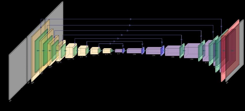
Super-resolving Herschel imaging 3

Table 1. Characteristics of the Herschel SPIRE and JCMT SCUBA-2 instruments. Confusion limits and PSF widths are from Nguyen et al. (2010), Wang et al.
(2017) and Dempsey et al. (2013).

 Characteristic Herschel SPIRE JCMT SCUBA-2

 Wavelength 250 µm 350 µm 500 µm 450 µm

 PSF FWHM 18.1" 24.9" 36.6" 7.9"

 Confusion noise ( , mJy/beam) 5.8 ± 0.3 6.3 ± 0.4 6.8 ± 0.4 1

 Pixel scale 6" 8.33" 12" 1"

3 NETWORK ARCHITECTURE of the network and its predictive performance on unseen input data
 (Ioffe & Szegedy 2015). For similar reasons, dropout layers are used
The generator network of the auto-encoder is based on that used by
 to randomly disable training 50% of the kernel weights in the first
the GalaxyGAN code (Schawinski et al. 2017). The CNN presented
 three layers of the decoder network (Srivastava et al. 2014).
in this paper differs from GalaxyGAN, and other previous works in
 The architecture of the CNN is described in table 2 and a schematic
two significant ways: (i) the use of a more computationally expensive
 shown in fig. 1. Using this architecture requires that the pixel dimen-
loss function, that is better designed to extract the individual features
 sions of the input and ouput images match. However, the Herschel
of interest, and (ii) no discriminator network is used.
 SPIRE 250 µm , 350 µm , and 500 µm image pixel scales are 6",
 The network processes the two training sets independently, in
 8.33", and 12" respectively, while the JCMT SCUBA-2 images have
succession. Each epoch4 begins by training on the entire simulated
 a pixel scale of 1". Accordingly, since the input and output images
training set, before training on the observed data set three times in
 represent equal areas on the sky, a 2-D linear interpolation routine
succession. The aim was to have the network learn the key structural
 from the SciPy Python package (Virtanen et al. 2020) was used to
features of the sub-mm images on the simulated data before using
 subsample the input Herschel images.
the observed data to fine-tune the network to handle any small differ-
ences between observed and simulated images. Each training set was
randomised before each run through the data. Due to simulation dif- 3.2 Loss Function
ferences in the flux distribution the observed data were renormalised
before training on them to ensure a comparable flux distribution to The common approach for deconvolution when designing the loss
the simulations. function for GANs (e.g. Schawinski et al. 2017; Moriwaki et al.
 2021) is to combine the loss disc from a discriminator network
 with a simple 1−loss between the encoder-decoder network output
3.1 Autoencoder predicted and a target image true .

The architecture presented in this paper uses a U-net configuration
(Ronneberger et al. 2015). The outputs from each convolutional layer = 1−loss + disc
 ∑︁
in the encoder network are concatenated with the inputs of their = | true − predicted | + disc (3)
corresponding layer in the decoder network. This helps to prevent the
overall network output from diverging substantially from its input. It The approach in this paper is different. While the CNN presented
takes as its input the three Herschel SPIRE bands (250 µm , 350 µm retains the 1−loss as part of the overall loss function, it is not the
and 500 µm ) images and is trained to produce an output image main component. The main goal of the CNN in this paper is to
that closely matches a target image consistent with the single JCMT super-resolve the sub-mm telescope PSF. To achieve this, a novel,
SCUBA-2 450 µm band. All activation functions in the CNN are custom loss function was designed to better target the data features
LeakyReLU: of interest. In particular, this multifaceted loss function focuses on the
 differences between the fluxes of any point sources that are identified
 ( in corresponding pairs of generated and target images.
 , < 0 The loss computation uses the Photutils Python package (Bradley
 ( ) = (1)
 , ≥ 0 et al. 2020) to identify point sources within the target or generated
 images and extract fluxes from circular apertures with 10 arcsec
except for the final layer where a sigmoid function is used:
 radius, centred on the identified source locations.
 1 The loss is computed by comparing the fluxes extracted from the
 ( ) = . (2)
 1 + − generated and target images, but the details of the computation are
 LeakyReLU was chosen as the activation functions over the ReLU different when training on the simulated and observed training sets.
function, as the zero-gradient nature of the ReLU function at < 0
can cause "dead neurons" in the network. The sigmoid function in the 3.2.1 Training on simulated data
final layer ensures a well constrained output range with continuous
coverage. Batch normalisation is included after each convolutional When the network is training on simulated data, the locations of
layer to regularise their outputs, which enhances the overall stability sources with signal-to-noise ratios of S/N > 3 are derived using
 the target image only. Fluxes are extracted from both the target and
 generated images using apertures corresponding to the target image
4 The term epoch refers to a complete pass over the combined observed and locations.
simulated training data sets. The loss is computed as the sum over all apertures of the absolute

 MNRAS 000, 1–12 (2021)

4 L. Lauritsen et al.

Table 2. Autoencoder network architecture. Layers 1-8 comprise the encoder, while layers 9-16 comprise the decoder. The output of the encoder network is a
2 × 2 × 512 element tensor embedding of the input image, which is used as the input to the decoder network. The outputs from each convolutional layer in the
encoder network are concatenated with the inputs of their corresponding layer in the decoder network. All layers use convolutional kernels 4 × 4 pixel extent in
the width and height dimensions. The output of layer 8 encodes the embedding for this auto-encoder network.

 Layer Input dimensions Kernels Part 1 Part 2 Part 3 Part 4 Activation Output dimension

 1 424 × 424 × 3 64 Conv. BatchNorm. LeakyReLU 212 × 212 × 64

 2 212 × 212 × 64 128 Conv. BatchNorm. LeakyReLU 106 × 106 × 128

 3 106 × 106 × 128 256 Conv. BatchNorm. LeakyReLU 53 × 53 × 256

 4 53 × 53 × 256 512 Conv. BatchNorm. LeakyReLU 27 × 27 × 512

 5 27 × 27 × 512 512 Conv. BatchNorm. LeakyReLU 14 × 14 × 512

 6 14 × 14 × 512 512 Conv. BatchNorm. LeakyReLU 7 × 7 × 512

 7 7 × 7 × 512 512 Conv. BatchNorm. LeakyReLU 4 × 4 × 512

 8 4 × 4 × 512 512 Conv. BatchNorm. LeakyReLU 2 × 2 × 512

 9 2 × 2 × 512 512 De-Conv. BatchNorm. Dropout Concat 7 LeakyReLU 4 × 4 × 1024

 10 4 × 4 × 1024 512 De-Conv. BatchNorm. Dropout Concat 6 LeakyReLU 7 × 7 × 1024

 11 7 × 7 × 1024 512 De-Conv. BatchNorm. Dropout Concat 5 LeakyReLU 14 × 14 × 1024

 12 14 × 14 × 1024 512 De-Conv. BatchNorm. Concat 4 LeakyReLU 27 × 27 × 1024

 13 27 × 27 × 1024 256 De-Conv. BatchNorm. Concat 3 LeakyReLU 53 × 53 × 512

 14 53 × 53 × 512 128 De-Conv. BatchNorm. Concat 2 LeakyReLU 106 × 106 × 256

 15 106 × 106 × 256 64 De-Conv. BatchNorm. Concat 1 LeakyReLU 256 × 256 × 128

 16 256 × 256 × 128 1 De-Conv. Sigmoid 424 × 424 × 1

Figure 1. Schematic of the autoencoder used in this work. The yellow boxes represent convolutional layers. The purple boxes represent de-convolutional layers.
The green boxes represent combined batch normalisation and LeakyReLU activation function layers. Blue boxes represent a sequence of batch normalisation,
dropout and LeakyReLU activation layers. The red box represents the sigmoid activation function in the final layer, and the grey boxes are the input/output
images.

 target
difference between the extracted flux in the target and generated where is the number of point sources that are identified in the
image. target
 target image, is the flux extracted from the th aperture in the
 generated
 target image and is the flux extracted from the th aperture
 target
 ∑︁
 in the generated image.
 sim target generated
 train = | − | (4)
 =1

MNRAS 000, 1–12 (2021)

Super-resolving Herschel imaging 5
3.2.2 Training on observed data 4 RESULTS
When the network is training on observed data, the locations of The CNN presented here was trained and tested using both a pure
source are derived for both the target and generated images. For the simulation data set and on a data set combining simulated and ob-
target image the source identification criterion remains S/N > 3, but served data. In Fig. 2 the performance on a pure simulation data set
for the generated image, this threshold is relaxed and all sources is demonstrated. The performance of the network on the combined
with S/N > 1 are identified. The disparity in S/N detection limits simulated and observed data can be seen in Fig. 3. It is clear that the
used originates in the different purposes of the loss function in the target images for the simulated data contain more discernible sources
two cases. When detecting sources in the real data the purpose is to than the real JCMT images do. This is likely due to the reduced noise
replicate the aperture flux in real galaxies. This necessitates that a in the simulated data. Figs. 2 and 3 show the Herschel bands, as
reasonable lower limit has to be set on sources that are attempted they are provided to the network, post-normalisation. The network
reconstructed. The opposite holds true when detecting sources in the has no effective way of recreating the noise inherent in real obser-
generated data. In this case it is just important to identify spurious flux vations. The median, and 1−loss components of the loss function,
anomalies that does not correspond to actual sources, necessitating a should drive the network to represent the mean noise level as a quasi-
lower S/N threshold. Four sets of fluxes are then extracted from both uniform background flux, the spatially varying nature of the real
the target and generated images using both sets of apertures. Fluxes data noise will not be reproduced. The noise in the real background-
are extracted from the target images using apertures from the target subtracted JCMT image is distributed around zero. This drives the
and generated images, and vice-versa. background level generated by the CNN to be very close to zero, but
 The loss is computed as it can never be negative because the sigmoid activation of the output
 target layer does not allow negative values. The enforced non-negativity of
 ∑︁
 
 observed 1 target generated the super-resolved image pixel values also means that the distribution
 train = target | − | of background noise is highly non-Gaussian and the significance of
 =1
 any point sources in the super-resolved image, relative to the back-
 generated
 ∑︁ generated ground level cannot be interpreted in a standard Gaussian framework.
 1 target− 
 + generated
 | | (5) The right-hand panel of Fig. 4 shows an Eddington-like bias in the
 =1 reconstructed fluxes at the faint end (Eddington 1913), caused by
 pre-selecting faint features in the reconstruction. The matching with
 generated
where is the number of point sources that are identified in the JCMT observations uses a lower threshold for features.
the generated image. The second term explicitly penalises spurious Fig. 5 shows the astrometric error on the predicted locations of all
features that appear in the generated image. of extracted sources detected in the super-resolved image. The natural
 intuition from single-dish observations is that the positional uncer-
 tainty of a point source should be approximately 0.6 FWHM /(S/N)
 where FWHM is the beam full-width half maximum and S/N is the
3.2.3 Common loss components
 signal-to-noise ratio of that source (e.g. Ivison et al. 2007). However,
In addition to those based on the aperture flux differences, three in this case, the reconstructed map is not a single-dish observation,
common components also contribute to training loss functions for even though it resembles one. The astrometric uncertainty is a non-
both the observational and simulated training datasets. The first is trivial product of the map reconstruction, and therefore it is some-
the reduced mean of the absolute per-pixel difference between the thing that must be determined directly from the comparison with the
target and generated images5 . truth data. A further complicating factor is that the pixel scales of
 the originally used Herschel SPIRE images are 6", 8.33" and 12",
 and that of the JCMT images is 1", while the network uses images
 pix
 1 1 ∑︁ target generated of the size 424 × 424 pixels. As 424 is not divisible by either of the
 train = | − | (6)
 pix Herschel SPIRE pixel scales, this will cause minor differences in the
 =1
 exact astrometric alignment of the images fed to the network causing
where pix is the number of pixels in either of the images. This small astrometric errors. Furthermore, the misalignment of the pixels
component ensures that the loss includes some influence from the in the Herschel SPIRE data, due to the individual pixel scales not
bulk of image pixels outside extracted apertures. being integer multiples of one another might cause additional issues.
 The second common loss component is the absolute difference However, we find that the astrometric accuracy is often better than
between the mean pixel fluxes of the generated and target images. the pixel scale of the Herschel SPIRE 500 µm images, which is the
This loss component is designed to encourage the generated image closest equivalent image to the JCMT SCUBA-2 images.
to have an integrated flux similar to that of the target image. Observed flux is a key characteristic of observed galaxies. A signif-
 Finally, the loss includes the absolute difference between the me- icant portion of the loss function was designed to target the recovery
dian pixel fluxes of the generated and target images. This component of this observable. Fig. 4 shows the relationship between the super-
is intended to produce generated images that have a similar distri- resolved fluxes and the target fluxes of all sources brighter than 10
bution of pixel intensities to the target images. Since the majority times the background flux RMS in the super-resolved image, for all
of image pixels are noise or background dominated, this tends to the test image pairs. To compute an absolute flux calibration for the
result in generated images with similar background properties to the super-resolved point-source fluxes, the JCMT SCUBA-2 450 µm and
targets. super-resolved images are both convolved with a 2D Gaussian with
 a FWHM of 36.3 arcsec. A mask is generated to isolate the bright-
 est pixels in the Herschel 500 µm image and the pixel fluxes at the
 unmasked locations are compared with corresponding pixel fluxes
5 This is often referred to as the L1 loss. in the two convolved images. Two linear scaling relations are found

 MNRAS 000, 1–12 (2021)

6 L. Lauritsen et al.

 Super-resolved (mJy/pixel) JCMT SCUBA-2 450 m (mJy/pixel)
 0.02 0.04 0.06 0.08 0.10 0.00 0.05 0.10 0.15 0.20

 200 200
 150 150
 100 100
 50 50
 Offset (arcsec)

 0 0
 50 50
 100 100
 150 150
 200 200
 200 100 0 100 200 200 100 0 100 200
 Offset (arcsec) Offset (arcsec)
 Herschel SPIRE 500 m Herschel SPIRE 350 m Herschel SPIRE 250 m
 200 200 200

 100 100 100
 Offset (arcsec)

 0 0 0

 100 100 100

 200 200 200
 200 100 0 100 200 200 100 0 100 200 200 100 0 100 200
 Offset (arcsec) Offset (arcsec) Offset (arcsec)
Figure 2. The performance of the CNN on simulated COSMOS data from Herschel SPIRE. Top left is the deconvolved image, top right is the actual JCMT
SCUBA-2 450 µm image, and the bottom row are the Herschel SPIRE images. The Herschel SPIRE images shown here are processed identically to the network
inputs. They are 2-D linearly interpolated, and linearly normalised to have pixel values between zero and unity. The simulated JCMT 450 µm image demonstrates
the depth that originates in the high S/N possible with simulations in the lack of discernible noise.

which map the pixel fluxes in the Herschel 500 µm image to those in ably extracted from super-resolved images. Note that the custom loss
the convolved JCMT SCUBA-2 450 µm and super-resolved images. function is designed to recover the total flux within a 10" aperture.
Finally, a direct calibration from the super-resolved image flux to the The pull is defined as = | − |/ , with being the expected
corresponding high-resolution is derived by concatenating these two value, being the mean value of the bin, and being the standard
linear mappings. deviation. The pull has been calculated for the reconstructed source
 While the network does seem to slightly underestimate the cali- fluxes in table 3, where it is shown that the pull for sources between 9
brated flux for the simulated sources, the results for observational and 24 mJy with only one exception varies between 0.11 and 0.65. A
data show good promise. It is worth noting that due to the sub- stacking of the reconstructed sources reveals that the reconstruction
stantial overlap between the sky areas covered by the individual test has a PSF profile very similar to that of the target data (see fig. 6).
images, many of the extracted fluxes correspond to the the same sub- This is achieved with only the 1−loss part of the loss function trying
mm galaxy, seen in a different image. Thus the source distribution to replicate the PSF shape.
might not be entirely representative. For bright sources identified in The completeness (also known as recall) and purity (also known
both the simulated and observational datasets, an approximately 1:1 as reliability) of the reconstructed sources are shown in fig. 7. Com-
correlation between the calibrated, super-resolved fluxes and their pleteness is defined as /( + ) where is the number
counterparts in the target images is evident, albeit with some scatter. of true positives and is the number of false negatives; purity is
This correlation implies that the fluxes of bright sources can be reli- /( + ) where is the number of false positives. Complete-

MNRAS 000, 1–12 (2021)

Super-resolving Herschel imaging 7

 Super-resolved (mJy/pixel) JCMT SCUBA-2 450 m (mJy/pixel)
 0.00 0.05 0.10 0.15 0.20 0.25 0.2 0.1 0.0 0.1 0.2

 2.52° 2.52°

 2.50° 2.50°

 2.48° 2.48°
 Dec (deg)

 2.46° 2.46°

 2.44° 2.44°

 2.42° 2.42°
 150.16°150.14°150.12°150.10°150.08° 150.16°150.14°150.12°150.10°150.08°
 RA (deg) RA (deg)
 Herschel SPIRE 500 m Herschel SPIRE 350 m Herschel SPIRE 250 m
 2.52° 2.52° 2.52°
 2.50° 2.50° 2.50°
 2.48° 2.48° 2.48°
 Dec (deg)

 2.46° 2.46° 2.46°
 2.44° 2.44° 2.44°
 2.42° 2.42° 2.42°
 150.16° 150.12° 150.08° 150.16° 150.12° 150.08° 150.16° 150.12° 150.08°
 RA (deg) RA (deg) RA (deg)
Figure 3. The performance of the CNN on real COSMOS data from Herschel SPIRE. Top left is the deconvolved image, top right is the actual JCMT SCUBA-2
450 µm image, and the bottom row are the Herschel SPIRE images. The Herschel SPIRE images shown here are processed identically to the network inputs.
They are 2-D linearly interpolated, and linearly normalised to have pixel values between zero and unity. The JCMT 450 µm image shows the noise inherent
in real observations, while the super-resolved image shows the power of an autoencoder in reconstructing the JCMT 450 µm image without the clear noise
contribution.

ness is evaluated considering a set of “real” sources with SNR ≥ 5 in 5 DISCUSSION
the JCMT SCUBA-2 450 µm STUDIES survey maps. Sources that
are detected in the generated maps are considered to be true positives While many comparable neural networks (e.g. Schawinski et al. 2017;
if they fall within 10" of a real source and false negatives otherwise. Jia et al. 2021; Moriwaki et al. 2021) use the output of a discriminator
On the other hand we evaluate purity by considering the set of all network as part of their loss functions this paper adopts a different
“potential” sources that are detected in the generated maps. Potential approach. Recall that the training objective of a discriminator com-
sources that fall within 10" of a real source are deemed to be true ponent in a GAN is to effectively distinguish between images that
positives and all other potential sources are counted as false posi- have been artificially generated or processed and images that are gen-
tives. The completeness is > 95% at sources brighter than 15 mJy, uine or pristine. However, in order to make this distinction, it may
and above 60% at 10 mJy. The purity does not drop below 87% at rely on features of the images that a human interpreter might con-
any point. Note that our reconstruction is remarkably complete even sider unimportant. In this paper, the most important objective from a
below the formal 500 µm blank-field confusion limit for Herschel human perspective is for the neural network to recover the locations
SPIRE (table 1). and fluxes of the genuine point sources in the target data. However,
 from the perspective of a CNN it may be that the data sets used in
 this paper (see Figs. 2 and 3) differ most significantly in their noise

 MNRAS 000, 1–12 (2021)

8 L. Lauritsen et al.

 Ideal reconstruction line Ideal reconstruction line
 102 Super-resolved Simulated Flux Super-resolved Observational Flux
 Super-resolved Aperture Flux (mJy)

 Super-resolved Aperture Flux (mJy)
 101 101

 100

 00 100 101 102 101
 Target Aperture Flux (mJy) Target Aperture Flux (mJy)

 100 101 102 100 101 102
 Number of Galaxies Number of Galaxies
Figure 4. Left panel: Comparison between fluxes of point sources that are detected in super-resolved simulated images and fluxes extracted from spatially
coincident point sources in simulated high resolution target images. Only sources with fluxes exceeding 10 times the background RMS in the super-resolved
image are considered. Note that the distribution of background noise is highly non-Gaussian and the significance of any point sources in the super-resolved
image, relative to the background level cannot be interpreted in a standard Gaussian framework. The flux is calculated using aperture photometry within a circular
aperture of 10" centered on the source locations. The grey histogram shows the number of sub-mm galaxies detected in each bin of target versus super-resolved
flux space. The red points and errors show the mean super-resolved aperture flux within each target flux bin and its associated standard deviation, respectively.
The bins are defined to ensure equal numbers of galaxies in each bin, which results in the faintest and brightest bins covering a large logarithmic range. The red
data points are located at the bin centres in logarithmic flux space. For clarity, the axes on the left panel are linear below 1 mJy and logarithmic above this value.
Right panel: Same as left-hand panel, but comparing observed high resolution JCMT SCUBA-2 450 µm images with super-resolved observed Herschel SPIRE
counterparts. Note the Eddington bias in the faint fluxes, caused by pre-selection on faint features in the reconstruction (see text).

characteristics. It is therefore possible that a discriminator network bands divides into each other, while the 8.33" of the 350 µm band
would realise its training objective more effectively by focusing its might cause some uncertainty in source location when the images are
attention on the fine details of the image noise, and disregarding the shifted during data augmentation. Finally, the redder sources might
point source properties like astrometry and flux. Conversely, by using have higher astrometric uncertainty as they are less represented in the
a hand engineered loss function, the network presented in this paper higher resolution Herschel bands. While further work might reduce
can be forced to focus on the image features that are most critical for this astrometric offset, Fig. 5 shows a tendency of astrometric preci-
the overall objective of super-resolving low resolution images. sion better than the 12" pixel scale of the 500 µm Herschel SPIRE
 Fig. 5 plots the offset distances and position angles between the band.
locations of identifiable point sources in the super-resolved Her- Following this successful proof of concept, there are several ob-
schel SPIRE data and the nearest sub-mm galaxy location in the vious next steps. These go beyond this initial analysis, and at least
corresponding JCMT SCUBA-2 imaging. Overall reconstruction ac- some of these will be presented in future papers.
curacy is excellent, with a purity calculated at above 87% at all Firstly, this deconvolution algorithm will be applied to all the
reconstructed source flux densities, and completeness above 95% at Herschel SPIRE extragalactic survey data sets. For deeper fields with
target source flux densities above 15 mJy. Nonetheless, some small richer multi-wavelength complementary data, the deconvolution can
offsets between the reconstructed and target source positions are ap- be compared to other approaches that use this supplementary data as
parent. These offsets are likely caused by the different pixel scales for a prior (e.g. Hurley et al. 2017; Serjeant 2019).
the different Herschel SPIRE bands, and the JCMT data. These pixel Secondly, there are enhancements that can be made to the simu-
scales are not exact multiples of each other and so pixels from the dif- lations, such as incorporating Galactic cirrus. Furthermore, Dunne
ferent image bands intercept flux from different parts of the sky, and et al. (2020) find that foreground large-scale structure can statistically
may encode information about different subsets of the true source magnify the background sub-mm source counts, so one improvement
distribution. Even after interpolation, the sources which fall close to the simulations would be to incorporate optical/near-infrared imag-
to the edge of a pixel in the lower resolution bands have inherently ing and the effects of weak lensing. The deconvolutions would then
uncertain positions, which is likely reflected in the CNN output. be able to make use of the three SPIRE bands and the optical/near-
Further, the uncertain alignment of in particular the 350 µm band infrared data. In the present analysis, the statistical clustering prop-
might cause problems. The 12" and 6" of the 500 µm and 250 µm erties of sub-mm galaxies are implicitly (and non-trivially) used to

MNRAS 000, 1–12 (2021)

Super-resolving Herschel imaging 9

 99%
 100

 80
 99%
 Angular Offset (arcsec)

 60

 40
 99%
 95%
 20
 68%

 0
 0 50 100 150 200 250 300 350
 Position Angle (degrees)

Figure 5. Angular distance versus position angle for offsets of extracted sources identified on the super-resolved images and the nearest counterpart point source
in coincident SCUBA-2 imaging. Position angles are defined in degrees anti-clockwise from West. Grey markers correspond with individual objects that are
identified in the super-resolved images. Contours showing the 68th, 95th and 99th percentiles are overlaid. Overall, the astrometric accuracy is excellent with
99% of the super-resolved objects having offsets . 15 arcseconds. There is some evidence for clustering of offsets to the Northwest.

reconstruct the missing Fourier modes on scales smaller than the is possible even in principle. Indeed, the balances between angular
point spread function (section 1), so simulating a wider range of resolution, point-source sensitivity and large-scale features are usu-
clustered multi-wavelength training data should improve the decon- ally explicit and deliberate choices in astronomical image processing,
volution. Strong gravitational lensing could also be included (e.g. driven in each case by the particular science goals (e.g. Briggs 1995;
Negrello et al. 2010), in which case the network could also encode Serjeant et al. 2003; Smith et al. 2019; Danieli et al. 2020). One
multi-wavelength information, such as the presence of a foreground could imagine optimising the loss function not just for completeness
elliptical or cluster to signpost possible strong lensing. Extending or reliability or some balance thereof, but instead to reproduce the
the simulations and neural net training to a wider multi-wavelength sub-mm galaxy source counts, or make the best estimate of the two-
domain has the potential in principle to implicitly incorporate more point correlation function of sub-mm galaxies, or reliably detect faint
information than explicit multi-wavelength priors, albeit at a cost of ultra-red sub-mm galaxies.
less direct interpretability.
 Thirdly, the loss function can be tailored to suit particular science
goals. The present analysis represents a particular balance between
 6 CONCLUSIONS
source completeness, source reliability, flux reproducibility and as-
trometric accuracy, but other choices are possible. There is no reason This paper has shown that it is possible to super-resolve Herschel
to suppose that a single "best" deconvolution to suit all purposes SPIRE data using CNNs. In this paper an autoencoder was chosen. A

 MNRAS 000, 1–12 (2021)

10 L. Lauritsen et al.

 JCMT SCUBA-2 450 m PSF
 1.0 Super-resolved PSF

 0.8

 0.6

 0.4

 0.2

 0.0

 0 5 10 15 20 25 30 35 40
 Arcsec

Figure 6. The stacked PSF of the real JCMT SCUBA-2 450 µm sources (blue), and the super-resolved sources (orange). The fluctuations in the real sources
originate from the small sample of real images that can be used for training and validation. This causes a large overlap of sky area repeating the same source
multiple times. The smoothness of the super-resolved PSF is achieved by the final activation layer suppressing the noise in the generated images.

new and innovative loss function was engineered to better replicate used in this work include the STUDIES program (program code
the image features of interest. M16AL006), archival data from the S2CLS program (program
 It is possible to reconstruct both astrometry and source flux using code MJLSC01) and the PI program of Casey et al. (2013, pro-
this method with some uncertainty. It is expected that the performance gram codes M11BH11A, M12AH11A, and M12BH21A). The James
on particularly the source flux would improve with a larger, more Clerk Maxwell Telescope is operated by the East Asian Observa-
varied training set of observed data, reducing the need for simulated tory on behalf of The National Astronomical Observatory of Japan;
data in the training phase. More realistic simulated data might also Academia Sinica Institute of Astronomy and Astrophysics; the Ko-
achieve this goal. rea Astronomy and Space Science Institute; Center for Astronom-
 Ultimately this method will allow for further exploration of the ical Mega-Science (as well as the National Key R&D Program of
fields observed by Herschel SPIRE as a complement to the observa- China with No. 2017YFA0402700). Additional funding support is
tions carried out with JCMT and similar telescopes. provided by the Science and Technology Facilities Council of the
 United Kingdom and participating universities and organizations in
 the United Kingdom and Canada. Additional funds for the construc-
 tion of SCUBA-2 were provided by the Canada Foundation for In-
ACKNOWLEDGEMENTS novation. The authors wish to recognize and acknowledge the very
 significant cultural role and reverence that the summit of Maunakea
We thank the anonymous referee for many thoughtful and help-
 has always had within the indigenous Hawaiian community. We are
ful comments that improved this paper. The sub-mm observations

MNRAS 000, 1–12 (2021)

Super-resolving Herschel imaging 11

 1.0
 Completeness 1.0
 Purity

 0.8 0.8

 0.6 0.6

 0.4 0.4

 0.2 0.2

 0.0 0.0
 0 5 10 15 20 25 0 5 10 15 20 25 30
 JCMT SCUBA-2 450 m source flux density (mJy) Reconstructed source flux density (mJy)
Figure 7. Left panel: Completeness of recreated sources inside 10" of detected SNR ≥ 5 sources in the JCMT SCUBA-2 450 µm STUDIES survey maps. Right
panel: Purity of sources detected in the reconstructed image as compared to sources with SNR ≥ 5 in the JCMT SCUBA-2 450 µm STUDIES survey. In both
cases, the horizontal axis shows the minimum flux density threshold under consideration. The shaded areas show the extent of the ±1 binomial uncertainties.

Table 3. The pull calculated for the reconstructed sources shown in the 1342222824, 1342222825, 1342222826, 1342222846, 1342222847,
righthand panel of fig. 4. 1342222848, 1342222849, 1342222850, 1342222851, 1342222852,
 1342222853, 1342222854, 1342222879, 1342222880, 1342222897,
 Flux (mJy) Pull 1342222898, 1342222899, 1342222900 and 1342222901.
 This research made use of Astropy,6 a community-developed core
 2.91 1.89 Python package for Astronomy (Astropy Collaboration et al. 2013,
 5.5 1.51 2018). This research made use of Photutils, an Astropy package
 for detection and photometry of astronomical sources (Bradley et al.
 6.36 1.22 2020). Data analysis made use of the Python packages Numpy (Harris
 7.39 0.79 et al. 2020), Scipy (Virtanen et al. 2020) and Pandas (The pandas
 development team 2020; Wes McKinney 2010) as well as Tensorflow
 8.47 1.55 (Abadi et al. 2015) in Keras (Chollet 2015). Figures were made with
 9.01 0.11 the Python package Matplotlib (Hunter 2007).
 SS and HD were supported in part by ESCAPE - The European
 9.77 0.64 Science Cluster of Astronomy & Particle Physics ESFRI Research
 11.03 0.43 Infrastructures, which in turn received funding from the European
 Union’s Horizon 2020 research and innovation programme under
 12.15 0.27 Grant Agreement no. 824064. SS and LL thank the Science and Tech-
 12.77 0.50 nology Facilities Council for support under grants ST/P000584/1 and
 ST/T506321/1 respectively.
 14.11 0.37

 15.47 1.02

 16.38 0.12 DATA AVAILABILITY
 19.61 0.55 The observational data used for this paper are the Herschel
 24.32 0.55 SPIRE COSMOS data, the maps for which can be down-
 loaded at https://irsa.ipac.caltech.edu/data/COSMOS/
 26.67 3.99 images/herschel/spire/, and the JCMT SCUBA-2 STUDIES
 data.

most fortunate to have the opportunity to conduct observations from
this mountain.
 This research has made use of data from HerMES project REFERENCES
(http://hermes.sussex.ac.uk/). HerMES is a Herschel Key Programme Abadi M., et al., 2015, TensorFlow: Large-Scale Machine Learning on Het-
utilising Guaranteed Time from the SPIRE instrument team, ESAC erogeneous Systems, http://tensorflow.org/
scientists and a mission scientist. The HerMES data was ac- Astropy Collaboration et al., 2013, A&A, 558, A33
cessed through the Herschel Database in Marseille (HeDaM - Astropy Collaboration et al., 2018, AJ, 156, 123
http://hedam.lam.fr) operated by CeSAM and hosted by the Bertin E., Fouqué P., 2010, SkyMaker: Astronomical Image Simulations
Laboratoire d’Astrophysique de Marseille. The OBSIDs of the Her- Made Easy (ascl:1010.066)
schel fields used were: 1342195856, 1342195857, 1342195858,
1342195859, 1342195860, 1342195861, 1342195862, 1342195863,
1342222819, 1342222820, 1342222821, 1342222822, 1342222823, 6 http://www.astropy.org

 MNRAS 000, 1–12 (2021)

12 L. Lauritsen et al.
Bradley L., et al., 2020, astropy/photutils: 1.0.0, Valiante E., et al., 2016, Monthly Notices of the Royal Astronomical Society,
 doi:10.5281/zenodo.4044744, https://doi.org/10.5281/zenodo. 462, 3146
 4044744 Viero M. P., et al., 2013, ApJ, 772, 77
Briggs D. S., 1995, in American Astronomical Society Meeting Abstracts. p. Virtanen P., et al., 2020, Nature Methods, 17, 261
 112.02 Vojtekova A., Lieu M., Valtchanov I., Altieri B., Old L., Chen Q., Hroch F.,
Casey C. M., et al., 2013, MNRAS, 436, 1919 2020, MNRAS, 503, 3204
Chollet F., 2015, Keras, https://github.com/fchollet/keras Wang W.-H., et al., 2017, ApJ, 850, 37
Clark C. J. R., et al., 2018, A&A, 609, A37 Wes McKinney 2010, in Stéfan van der Walt Jarrod Millman eds, Pro-
Danieli S., et al., 2020, ApJ, 894, 119 ceedings of the 9th Python in Science Conference. pp 56 – 61,
Dempsey J. T., et al., 2013, MNRAS, 430, 2534 doi:10.25080/Majora-92bf1922-00a
Dudzevičiūtė U., et al., 2020, MNRAS, 494, 3828
Dunne L., Bonavera L., Gonzalez-Nuevo J., Maddox S. J., Vlahakis C., 2020, This paper has been typeset from a TEX/LATEX file prepared by the author.
 MNRAS, 498, 4635
Eales S., et al., 2010, PASP, 122, 499
Eddington A. S., 1913, MNRAS, 73, 359
Franco M., et al., 2018, A&A, 620, A152
Geach J. E., et al., 2013, Monthly Notices of the Royal Astronomical Society,
 432, 53
Geach J. E., et al., 2017, MNRAS, 465, 1789
Goodfellow I. J., Pouget-Abadie J., Mirza M., Xu B., Warde-Farley D., Ozair
 S., Courville A., Bengio Y., 2014, Generative Adversarial Networks
 (arXiv:1406.2661)
Goodfellow I., Bengio Y., Courville A., 2016, Deep Learning. MIT Press
Greenslade J., et al., 2018, Monthly Notices of the Royal Astronomical Soci-
 ety, 476, 3336
Griffin M. J., et al., 2010, A&A, 518, L3
Harris C. R., et al., 2020, Nature, 585, 357
Hayward C. C., Narayanan D., Kereš D., Jonsson P., Hopkins P. F., Cox T. J.,
 Hernquist L., 2013, MNRAS, 428, 2529–2547
Hodge J. A., et al., 2013, ApJ, 768, 91
Holland W. S., et al., 2013, MNRAS, 430, 2513
Hunter J. D., 2007, Computing in Science & Engineering, 9, 90
Hurley P. D., et al., 2017, MNRAS, 464, 885
Ioffe S., Szegedy C., 2015, Batch Normalization: Accelerating Deep Network
 Training by Reducing Internal Covariate Shift (arXiv:1502.03167)
Ivison R. J., et al., 2007, MNRAS, 380, 199
Jia P., Ning R., Sun R., Yang X., Cai D., 2021, MNRAS, 501, 291
Jin S., et al., 2018, ApJ, 864, 56
Levenson L., et al., 2010, MNRAS, 409, 83
Lewis A. J. R., et al., 2018, The Astrophysical Journal, 862, 96
Lutz D., 2014, ARA&A, 52, 373
Ma C.-J., et al., 2015, The Astrophysical Journal, 806, 257
Moriwaki K., Shirasaki M., Yoshida N., 2021, The Astrophysical Journal,
 906, L1
Negrello M., et al., 2010, Science, 330, 800
Nguyen H. T., et al., 2010, Astronomy and Astrophysics, 518, L5
Oliver S. J., et al., 2010, A&A, 518, L21
Oliver S. J., et al., 2012, MNRAS, 424, 1614
Pilbratt G. L., et al., 2010, A&A, 518, L1
Ronneberger O., Fischer P., Brox T., 2015, in Navab N., Hornegger J., Wells
 W. M., Frangi A. F., eds, Medical Image Computing and Computer-
 Assisted Intervention – MICCAI 2015. Springer International Publishing,
 Cham, pp 234–241
Schawinski K., Zhang C., Zhang H., Fowler L., Santhanam G. K., 2017,
 Monthly Notices of the Royal Astronomical Society: Letters, 467, L110
Schreiber C., et al., 2017, A&A, 602, A96
Serjeant S., 2019, Research Notes of the American Astronomical Society, 3,
 133
Serjeant S., et al., 2003, MNRAS, 344, 887
Simpson J. M., et al., 2015, ApJ, 799, 81
Smith M. W. L., et al., 2019, MNRAS, 486, 4166
Srivastava N., Hinton G., Krizhevsky A., Sutskever I., Salakhutdinov R.,
 2014, Journal of Machine Learning Research, 15, 1929
Starck J., Pantin E., Murtagh F., 2002, Publications of the Astronomical
 Society of the Pacific, 114, 1051
The pandas development team 2020, pandas-dev/pandas: Pandas,
 doi:10.5281/zenodo.3509134, https://doi.org/10.5281/zenodo.
 3509134

MNRAS 000, 1–12 (2021)