VariantStore: an index for large-scale genomic variant search
←
→
Page content transcription
If your browser does not render page correctly, please read the page content below
Pandey et al. Genome Biology     (2021) 22:231
https://doi.org/10.1186/s13059-021-02442-8

 METHOD                                                                                                                                         Open Access

VariantStore: an index for large-scale
genomic variant search
Prashant Pandey, Yinjie Gao and Carl Kingsford*

*Correspondence:
carlk@cs.cmu.edu                         Abstract
Computational Biology
Department, School of Computer
                                         Efficiently scaling genomic variant search indexes to thousands of samples is
Science, Carnegie Mellon University,     computationally challenging due to the presence of multiple coordinate systems to
Pittsburgh, USA                          avoid reference biases. We present VariantStore, a system that indexes genomic
                                         variants from multiple samples using a variation graph and enables variant queries
                                         across any sample-specific coordinate system. We show the scalability of VariantStore
                                         by indexing genomic variants from the TCGA project in 4 h and the 1000 Genomes
                                         project in 3 h. Querying for variants in a gene takes between 0.002 and 3 seconds using
                                         memory only 10% of the size of the full representation.
                                         Keywords: Variation graph, Graph genomes, Pangenomes

                                       Background
                                       Advanced sequencing technology and computing resources have led to large-scale
                                       genomic sequencing efforts producing genomic variation data from thousands of sam-
                                       ples, such as the 1000 Genomes project [1–3], GTEx [4], and The Cancer Genome Atlas
                                       (TCGA) [5]. Analysis of genomic variants combined with phenotypic information of sam-
                                       ples promises to improve applications such as personalized medicine, population-level
                                       disease analysis, and cancer remission rate prediction. Although numerous studies [6–12]
                                       have been performed over the past decade involving genomic variation, the ability to scale
                                       these studies to large-scale data available today and in the near future is still limited.
                                          On an individual sample, the typical result of sequencing, alignment, and variant calling
                                       is a collection of millions of sample-specific variants. A variant is identified by the position
                                       in the chromosome where it occurs, an alternative sequence, a list of samples that contain
                                       the variant, and phasing information. The standard file format to report these variants is
                                       the variant call file (VCF) [13].
                                          Traditional reference-based variant storing methods, like VCF, store variants based on
                                       a single reference coordinate system and therefore have certain limitations. The choice
                                       of reference introduces reference bias in mapping, variant calling, and downstream anal-
                                       ysis [14]. It leads to the misinterpretation of the “reference” as a baseline, while in fact it

                                       © The Author(s). 2021 Open Access This article is licensed under a Creative Commons Attribution 4.0 International License,
                                       which permits use, sharing, adaptation, distribution and reproduction in any medium or format, as long as you give appropriate
                                       credit to the original author(s) and the source, provide a link to the Creative Commons licence, and indicate if changes were
                                       made. The images or other third party material in this article are included in the article’s Creative Commons licence, unless
                                       indicated otherwise in a credit line to the material. If material is not included in the article’s Creative Commons licence and your
                                       intended use is not permitted by statutory regulation or exceeds the permitted use, you will need to obtain permission directly
                                       from the copyright holder. To view a copy of this licence, visit http://creativecommons.org/licenses/by/4.0/. The Creative
                                       Commons Public Domain Dedication waiver (http://creativecommons.org/publicdomain/zero/1.0/) applies to the data made
                                       available in this article, unless otherwise stated in a credit line to the data.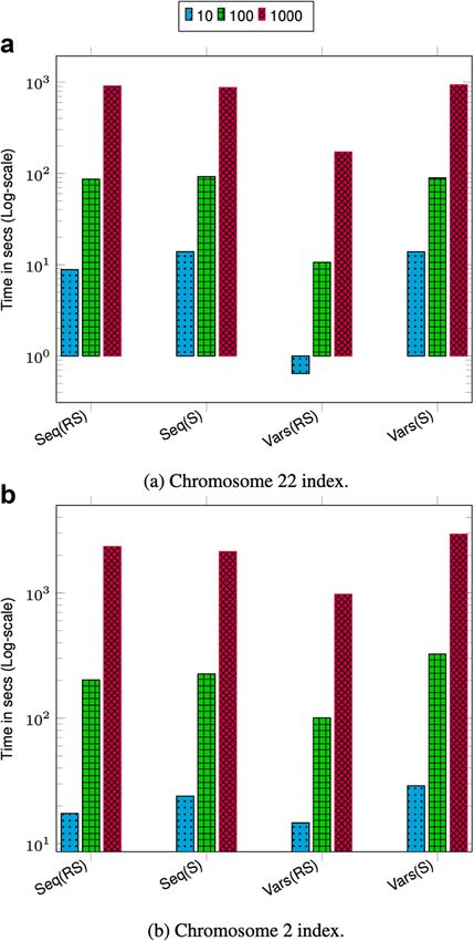
Pandey et al. Genome Biology    (2021) 22:231                                                                   Page 2 of 25

                 is mostly a type specimen [14]. Storing highly variant sequence repertoires can be chal-
                 lenging because choosing a single representative sequence as reference is no longer viable
                 and a bad choice of reference could lead to inefficient storage. For example, regions with
                 high diversity, like T cell receptors (TCR), of which one person could have 1013 different
                 clonotypes [15], are stored in a pan-genomic structure to preserve diversity.
                    A primary goal of pan-genomic variation analysis is to avoid biases that arise when
                 treating a single genome as the reference when identifying or comparing variants across
                 samples [16, 17]. In pan-genomic variation analysis, we can identify and study variants
                 based on any sample genome and compare variants from two samples directly without the
                 need for a distinguished reference genome. The ability to compare samples directly also
                 enables the comparison of variants derived from samples belonging to different species.
                 Comparing variants from closely related species is often critical to study the evolution-
                 ary and mechanistic relationships between plant genomes that evolve quickly to adapt to
                 external environments [18–21].
                    We present VariantStore, a system for efficiently indexing and querying genomic
                 information (genomic variants and phasing information) from thousands of samples con-
                 taining millions of variants. VariantStore supports querying variants occurring between
                 two positions across a chromosome based on any sample coordinate system. Specifically,
                 VariantStore supports queries of the following types:
                    •   Find the closest variant to position X in sample S coordinates
                    •   Find the sequence between positions X and Y for sample S1 in sample S2 coordinates
                    •   Find all variants between positions X and Y for sample S1 in sample S2 coordinates
                    •   Find all variants between positions X and Y in sample S coordinates

                   The positions specified in variant queries are based on a coordinate system that
                 uniquely identifies the positions of variants in a given genome [22]. Each sample in the
                 input data can have a different coordinate system due to the presence of insertions and
                 deletions (indels). In any of the above queries, the sample S used for the coordinate space
                 can be any of the samples present in the system. If the collection of samples includes a
                 standard reference genome (such as GRCh37), the queries can be presented using that
                 coordinate system. If a known region in a particular sample is of interest, the queries can
                 be presented in that sample’s coordinates. Particularly usefully, if the collection contains
                 two “reference” genomes (such as GRCh37 and GHCh38), queries can be posed in either
                 of those coordinate systems. This avoids the effort of calling variants on all the existing
                 samples based on the new reference [23].
                   Supporting variant queries based on multiple sample coordinate systems requires main-
                 taining a function per sample that can map a position in the reference coordinate (as
                 present in VCF files) to the sample coordinate. Maintaining thousands of such functions
                 requires storing and accessing an order of magnitude more data than only indexing vari-
                 ants based on a single reference coordinate system. Efficiently supporting thousands of
                 coordinate systems adversely affects the memory footprint and computational complex-
                 ity of the system making this problem much more challenging. This limits the scalability
                 of variant indexes that support multiple coordinate systems to variation data containing
                 only a few thousands samples.
                   VG toolkit [24] is one of the most widely used tools to represent genomic variation data,
                 and it also supports multiple coordinate systems. It encodes genomic variants from mul-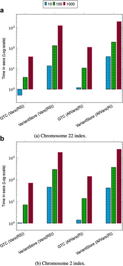
Pandey et al. Genome Biology   (2021) 22:231                                                                      Page 3 of 25

                 tiple samples in a graph, called a variation graph. A variation graph is a sequence graph
                 [25] where each node represents a sequence and a set of nodes through the graph, known
                 as a path, embeds the complete sequence corresponding to each sample. Each node on
                 a path is assigned a position indicating the location of the sequence in the coordinate
                 system of the path. A node can be assigned multiple positions based on the number of
                 paths that pass through the node. The variation graph enables read alignment against
                 multiple sample sequences containing variants simultaneously and avoids mapping biases
                 that arise when mapping reads to a single reference sequence [24, 26–31].
                    VG toolkit stores each sample path as a list of nodes in the graph and maintains a
                 separate index corresponding to the coordinates of the reference and samples. Storing a
                 separate list of nodes for each sequence impedes the scalability of the representation for
                 storing variation from thousands of samples. Moreover, variants are often shared among
                 samples, so storing a list of nodes for each sample path introduces redundancy in the rep-
                 resentation. VG toolkit is designed to optimize read alignment and uses sequence-based
                 indexes for alignment [32, 33]. It cannot be directly used for variant queries that require an
                 index based on the position of variants in multiple sequence coordinates. Finally, the VG
                 toolkit representation does not store phasing information contained in VCF files, which
                 is required in many analyses.
                    Multiple solutions have been proposed that efficiently index variants and support a sub-
                 set of the variant queries described above. GQT [34] was the first tool that proposed a
                 sample-centric index for storing and querying variants. It stores variants in compressed
                 bitmap indexes and supports efficient comparisons of sample genotypes across many
                 variant positions. BGT [35] and GTC [36] proposed variant-centric indexes that store
                 variants in compressed bit matrices. They support queries for variants in a given region
                 and allow filtering returned variants based on subsets of samples. The SeqArray library
                 [37] is another variant-centric tool for the R programming language to store and query
                 variants.
                    However, these tools index variants only in the reference coordinate system and do not
                 support variant queries in a sample coordinate system. Supporting multiple coordinate
                 systems is a much harder problem. Furthermore, these tools do not store the reference
                 sequence and cannot be directly used to query and compare sample sequences in a given
                 region. Other tools have been proposed that use traditional database solutions, such as
                 SQL and NoSQL [38–40]. However, they have proven prohibitively slow to index and
                 query collections of variants.
                    VariantStore bridges the gap between the tools that are space-efficient and fast but only
                 support reference-based queries (e.g., GTC [36]) and VG, which maintains multiple coor-
                 dinate systems by storing variants in a variation graph but fails to scale to thousands of
                 samples. We show this by indexing variants from both the 1000 Genomes and TCGA
                 projects (> 8K samples) and show that VariantStore is faster than VG and takes less mem-
                 ory and disk space. VariantStore performs variant queries based on sample coordinates in
                 less than a second. Furthermore, we have designed VariantStore to efficiently scale out of
                 RAM to storage devices in order to cater to the ever increasing sizes of available variation
                 data by performing memory-efficient construction and query.
                    We encode genomic variation in a directed, acyclic variation graph and build a position
                 index (a mapping of node positions to node identifiers) on the graph to quickly access a
                 node in the graph corresponding to a queried position. Each node in the variation graph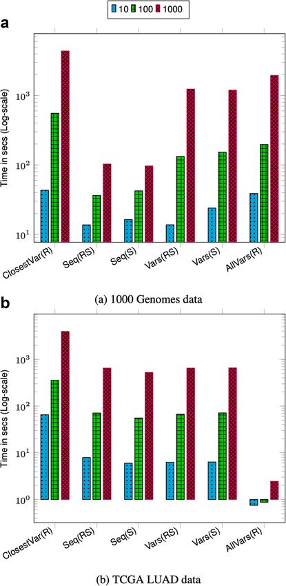
Pandey et al. Genome Biology   (2021) 22:231                                                                   Page 4 of 25

                 corresponds to a variant and stores a list of samples that contain the variant along with
                 the position of the variant in the coordinate of those samples. The inverted index design
                 allows one to quickly find all the samples and positions in sample coordinates correspond-
                 ing to a variant. It also avoids redundancy that otherwise arises in maintaining individual
                 variant indexes for each sample coordinate and scales well in practice when the number
                 of samples grows beyond a few thousand.
                   To efficiently scale to thousands of coordinate systems (or samples), we maintain the
                 position index only on a single sample coordinate system (often the reference genome in
                 the input VCF). The position index maps positions in the sample sequence where there is
                 a variant to nodes corresponding to those variants in the variation graph. The sequence
                 chosen for the position index is called the marker sequence and the nodes on the path
                 of the marker sequence act as marker nodes in the variation graph. To lookup a position
                 using a sample’s coordinate system, we first lookup the marker node corresponding to the
                 position in the marker sequence using the position index. We then traverse the sample
                 path from the marker node in the graph to determine the appropriate node in the sample
                 coordinate. A node with a given position in a sample coordinate is often close to the node
                 in the marker sequence coordinate with the same position.
                   Maintaining the position index only on the marker sequence also makes it easier to
                 include multiple references in the same index. Each new reference can be treated as a
                 sample. Adding a new reference sequence to the index requires adding the variation in the
                 new reference based on the previous reference already in the index. Furthermore, to speed
                 up searches based on the new reference, one can also add a new position index mapping
                 the nodes corresponding to the new reference. We can then use the new position index to
                 directly locate nodes corresponding to positions in the coordinate of the new reference. By
                 enabling queries in any sample’s coordinate system, we eliminate the artificial dichotomy
                 between predetermined reference sequences and other samples.
                   To perform index construction and query efficiently in terms of memory, we partition
                 the variation graph into small chunks (usually a few MBs in size) based on the marker
                 sequence coordinates and store variation graph nodes in these chunks. During construc-
                 tion, only the active chunk is maintained in memory in which new nodes are added,
                 and once it reaches its capacity, we compress and serialize it to disk and create a new
                 active chunk. The nodes in and across chunks are ordered based on the marker sequence
                 coordinate. During a query, we only load the chunks in memory that contain the nodes
                 corresponding to the query range. VariantStore can control the memory usage by tun-
                 ing the chunk size. This enables VariantStore to scale to very large datasets even on
                 commodity machines where the working memory is often scarce.

                 Results
                 Our evaluation of VariantStore is based on four parameters: construction time, query
                 throughput, disk space, and peak memory usage.
                   To calibrate our performance numbers, we compare VariantStore against VG toolkit
                 [41]. VG toolkit represents variants in a variation graph and supports multiple coordi-
                 nate systems similar to VariantStore but does not support variant queries. Therefore, we
                 use the VG toolkit representation as a baseline for space usage and construction time in
                 our evaluation as it stores the same information as the VariantStore. The main difference
                 between VariantStore and the VG toolkit is that VG toolkit uses a separate index corre-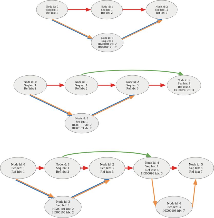
Pandey et al. Genome Biology   (2021) 22:231                                                                   Page 5 of 25

                 sponding to each coordinate system whereas VariantStore stores a single index of marker
                 nodes in the variation graph. Comparison with VG toolkit also allows us to evaluate the
                 scalability of existing variation graph indexing tools to index variants from thousands to
                 samples. We do not include VG toolkit in our query evaluation as it does not support the
                 variant queries supported by VariantStore.

                 Data
                 We use 1000 Genomes Phase 3 data [42] and three of the biggest projects from TCGA in
                 terms of the number of samples, Ovarian Cancer (OV), Lung Adenocarcinoma (LUAD),
                 and Breast Invasive Carcinoma (BRCA), for our evaluation. 1000 Genomes data contains
                 more variants compared to the TCGA data but TCGA data contains more samples. 1000
                 Genomes data contains a separate VCF file for each chromosome containing variants
                 from thousands of samples. The number of samples in each file is ≈ 2.5K. The variants in
                 1000 Genomes project are based on GRCh37 reference genome. The TCGA data contains
                 a multiple separate VCF files. The OV, LUAD, and BRCA projects contain 2436, 2680,
                 and 4319 VCF files, respectively. Each VCF file contains two variant types: normal and
                 tumor. For each project in TCGA, we first merged VCF files using the BCF tool merge
                 command [43] and created a separate VCF file for each chromosome. The variants in the
                 TCGA project are based on GRCh38 reference genome.

                 Index construction
                 The total time taken to construct the variation graph representation and index includes
                 the time taken to read and parse variants from the VCF file, construct the variation
                 graph representation and indexes, and serialize the final representation to disk. For Vari-
                 antStore, the reported time includes the time to create and serialize the position index.
                 The space reported for VariantStore is the sum of the space of the variation graph
                 representation and position index.
                   For VG toolkit, creating a variation graph representation with multiple coordinate sys-
                 tems (or sample path annotations) requires creating two indexes, XG and GBWT index.
                 The XG index is a succinct representation of the variation graph without path annotations
                 that allows memory- and time-efficient random access operations on large graphs. The
                 GBWT (graph BWT) is a substring index for storing sample paths in the variation graph.
                 We first create the variation graph representation using the “construct” command includ-
                 ing all sample path annotations. We then create the XG index and GBWT index from the
                 variation graph representation to create an index with all sample path annotations in the
                 variation graph. For VG toolkit, the reported time includes the time to create and serial-
                 ize the XG and GBWT indexes. The space reported for VG toolkit is the sum of the space
                 of the XG and GBWT indexes. VG toolkit could not build GBWT index on TCGA data
                 even after running for more than a day. We only report space for the XG index (which
                 does not contain any sample path annotations) for TCGA data.
                   For both VariantStore and VG toolkit, we created 24 separate indexes, one each for
                 chromosomes 1–22 and X and Y. Each of these indexes were constructed in parallel as
                 a separate process. We report the time taken for construction as the time taken by the
                 process that finished last. Index construction was slowest for chromosome 2 in 1000
                 Genomes data for both VG toolkit and VariantStore. In TCGA data, chromosome 1 was
                 the slowest. For disk space, we report the total space taken by all 24 indexes. For peak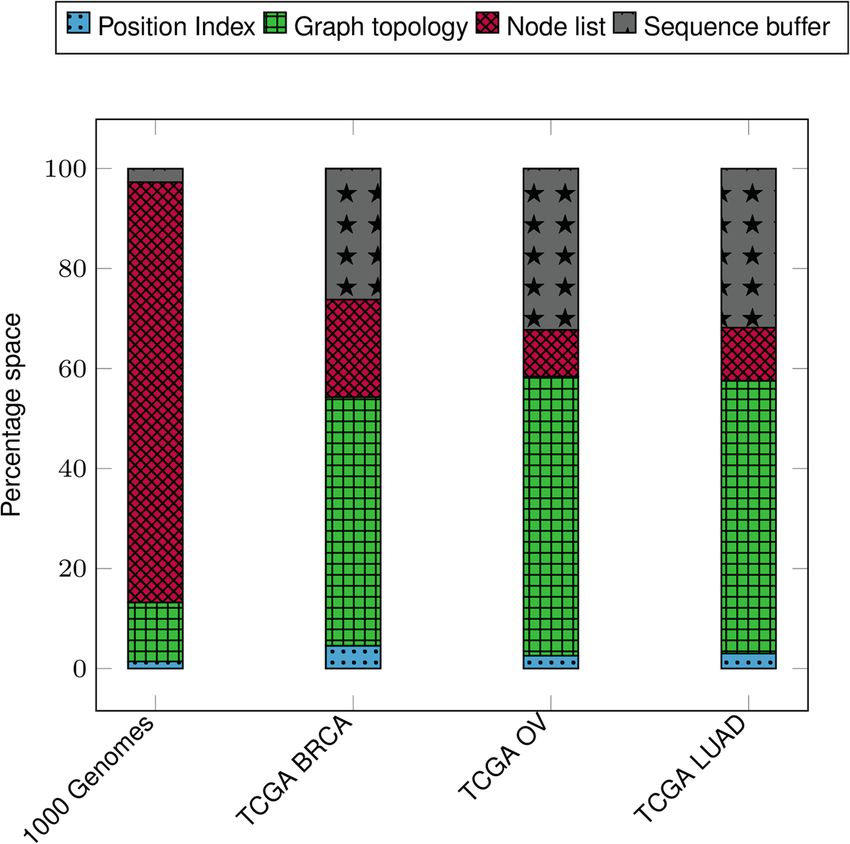
Pandey et al. Genome Biology       (2021) 22:231                                                                     Page 6 of 25

                 memory usage, we report the highest individual and aggregate peak RAM usage for all
                 processes.
                   The performance of VariantStore and VG toolkit for constructing the index on the 1000
                 Genomes and TCGA data is shown in Table 1.
                   VariantStore is 3× faster, takes 25% less disk space, and 3× less peak RAM than VG
                 toolkit. For the TCGA data, VG toolkit could not build GBWT index embedding all sam-
                 ple paths. However, even the space needed for the XG index (not embedding sample
                 paths) is ≈ 3.3× larger than the VariantStore representation containing all sample paths.

                 Query throughput
                 We measured the query throughput for all four query types mentioned above. To show
                 the robustness of query efficiency on different data, we evaluate on two different chromo-
                 some indexes from two different projects. We chose chromosome 2 which is one of the
                 bigger chromosomes and chromosome 22 which is one of the smaller ones. We evaluate
                 query time on chromosome indexes from 1000 Genomes and TCGA LUAD data.
                   To perform queries, we specify a pair of positions in a sample coordinate system
                 depending on the query type and a sample name. To evaluate the effect of querying based
                 on a sample other than the marker sequence (reference sequence), we perform two types
                 of queries, finding the sequence in a region and finding the variants in a region, using both
                 the marker sequence and a random sample from the input VCF. Specifically, we perform
                 the following six types of queries:

                    1      ClosestVar(R ; X ): closest variant to X in the marker sequence coordinates
                    2      Seq(R, S ; X, Y ): sequence for sample S between X and Y in the marker sequence
                           coordinates
                    3      Seq(S ; X, Y ): sequence for sample S between X and Y in its coordinates
                    4      Vars(R, S ; X, Y ): variants for sample S between X and Y in the marker sequence
                           coordinates

                 Table 1 Time, space, peak RAM, and peak RAM (aggregate) to construct variant index on the 1000
                 Genomes and TCGA (OV, LUAD, and BRCA) data using VariantStore and VG toolkit. ∗ VG toolkit could
                 not build GBWT index embedding all sample paths for TCGA data. Space reported is for the XG index
                 that does not contain any path information. We constructed all 24 chromosomes (1–22 and X and Y)
                 in parallel. The time and peak RAM reported is for the biggest chromosome (usually chromosome 1
                 or 2). The space reported is the total space on disk for all 24 chromosomes. The peak RAM
                 (aggregate) is the aggregate peak RAM for all 24 processes
                 System                     Time            Disk space            Peak RAM         Peak RAM Agg.
                 Dataset                                             1000 Genomes
                    VariantStore            3 h 25 min      41 GB                 8.8 GB           153 GB
                    VG toolkit              11 h 10 min     50 GB                 37 GB            450 GB
                 Dataset                                                  TCGA (OV)
                    VariantStore            1 h 5 min       3.4 GB                1.1 GB           17.45 GB
                    VG-toolkit                              11 GB∗
                 Dataset                                                 TCGA (LUAD)
                    VariantStore            1 h 20 min      3.5 GB                2.3 GB           36.05 GB
                    VG toolkit                              12 GB∗
                 Dataset                                                 TCGA (BRCA)
                    VariantStore            4 h 36 min      4.2 GB                3.2 GB           53.21 GB
                    VG toolkit                              14 GB∗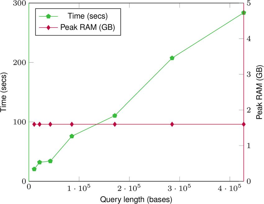
Pandey et al. Genome Biology (2021) 22:231 Page 7 of 25
5 Vars(S ; X, Y ): variants for sample S between X and Y in its coordinates
6 AllVars(R ; X, Y ): all variants between X and Y in the marker sequence coordinates
VariantStore supports ClosestVar(S;X) and AllVars(S;X, Y ) for any S. In our experiments,
we present results for S equal to the marker sequence for those queries because they are
representative of the performance of those queries.
During a query, we only load the position index and graph topology completely in mem-
ory which are only a small portion of the total index space. The nodes in the variation
graph representation are partitioned into chunks and only relevant chunks correspond-
ing to the query range are loaded in memory. Keeping the variation graph representation
on disk keeps the peak memory usage low and all disk accesses are performed during the
query to load appropriate node chunks.
Given a batch of queries, we first sort the queries based on the starting position (treating
input positions in the marker coordinate system for all query types) and then perform
the queries in order. Performing queries in sorted order ensures that we always access
node chunks in sequential order and only have to load a chunk once to answer all queries
corresponding to the range of nodes it contains. It also amortizes the cost of loading and
unloading node chunks to and from disk.
We performed three sets of query benchmarks containing 10, 100, and 1000 queries and
report the aggregate time. For each query in the set, we uniformly randomly pick the start
position across the full chromosome length. The size of the query range is set to ≈ 42K
bases which is approximately the length of a typical gene. Picking multiple query regions
uniformly randomly across the chromosome provides a good coverage of different regions
across the chromosome.
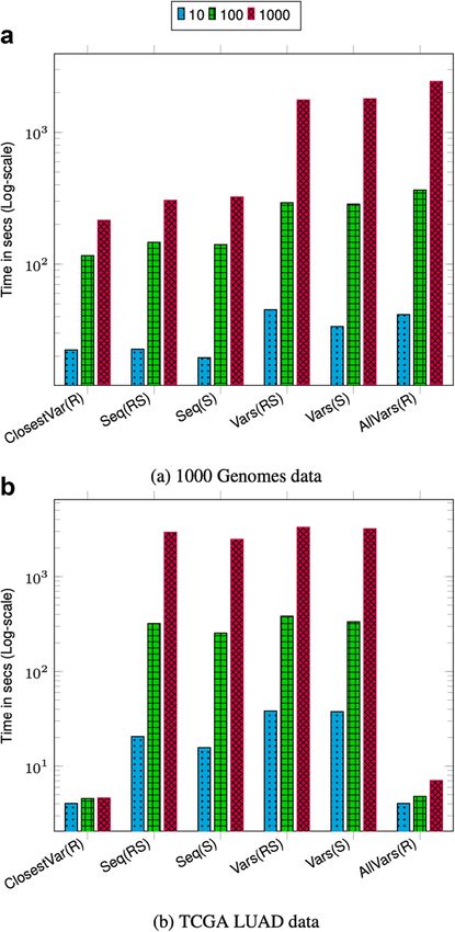
The query throughput on 1000 Genomes data is shown in Figs. 1a and 2a. For most
query types, the aggregate time taken to execute queries increases sublinearly with the
number of queries. This is because as the batch size increases the cost of loading and
unloading node chunks is amortized against higher number of queries. Finding the
sequence corresponding to a sample in a region (Seq(RS) and Seq(S)) takes less time
compared to finding variants in a region (Vars(RS), Vars(S), and AllVars(R)). Finding the
sequence takes less time because it involves traversing the sequence specific path in the
region and reconstructing the sequence. However, finding variants in a given region takes
more time because it involves an exhaustive search of neighbors at each node in the region
to determine all the variants that are contained by a given sample or all samples.
The query throughput on TCGA data is shown in Figs. 1b and 2b. The TCGA data has
twice as many samples compared to 1000 Genomes data but there are fewer variants. This
makes the variation graph much sparser and queries in the position index become more
expensive compared to traversing the graph between two positions. Finding all variants is
the fastest query because the variation graph is very sparse and most position ranges are
empty. Traversing the graph to find the sequence or variants for a sample takes similar
amount of time. Finding the closest variant from a position takes the most amount of time
because it involves performing multiple position index queries to determine the closest
variant.
For both 1000 Genomes and TCGA LUAD data, finding the closest variant query is
faster for chromosome 2 because variants in chromosome 22 are more dense compared
to chromosome 2 which makes it faster to locate the closest variant.Pandey et al. Genome Biology (2021) 22:231 Page 8 of 25
Fig. 1 Chromosome 22 query performance. Time reported is the total time taken to execute 10, 100, and
1000 queries. For all queries, the query length is fixed to ≈ 42K. ClosestVar(R), Closest variant; Seq(RS), Seq in
ref coordinate; Seq(S), Seq in Sample coordinate; Vars(RS), Sample variants in ref coordinate; Vars(S), Sample
variants in Sample coordinate; AllVars(R), All variants in ref coordinate
The effect of querying based on a sample other than the marker sequence is negligible
as shown in the timing results for Seq(RS) and Seq(S) and query Vars(RS) and Vars(S).
This shows that the overhead of the local graph search to convert the position from the
coordinate of the marker sequence to the sample sequence is low.
The effect of query range on peak memory usage
We performed another query benchmark to evaluate the effect of size of the position
range on the peak memory usage and time. For this benchmark, we chose the “Sample
sequence in marker coordinate” query (Seq(RS)) because this query involves travers-
ing the full sample path between two positions. We performed sets of 100 queries withPandey et al. Genome Biology (2021) 22:231 Page 9 of 25
Fig. 2 Chromosome 2 query performance. Time reported is the total time taken to execute 10, 100, and 1000
queries. For all queries the query length is fixed to ≈ 42K. ClosestVar(R), Closest variant; Seq(RS), Seq in ref
coordinate; Seq(S), Seq in Sample coordinate; Vars(RS), Sample variants in ref coordinate; Vars(S), Sample
variants in Sample coordinate; AllVars(R), All variants in ref coordinate
increasing size of the position range and record the total time and peak RAM usage.
For each query in the set, we uniformly randomly pick the start position across the full
chromosome length.
The effect of the query range size on peak memory usage and time is shown in Fig. 3.
The memory usage remains constant regardless of the query length. This is because dur-
ing a query we access node chunks in sequential order and regardless of the query length
only load at most two node chunks in RAM at a time. This keeps the memory usage
essentially constant.Pandey et al. Genome Biology (2021) 22:231 Page 10 of 25
Fig. 3 Time (seconds) and peak memory usage (GB) with increasing query length for “Sample sequence in
the marker coordinate” (Seq(RS)) for 1000 Genomes chromosome 22 index. The time taken increases as the
query length increases. But the memory usage remains constant regardless of the query length
The peak memory usage depends on the size of node chunks and is not a hard con-
straint. It can be tuned to a lower or higher value depending on the system requirements
by changing the size of node chunks.
The effect of number of variants on query time
We also evaluate how the number of variants in the position range affects the query time.
For this benchmark, we performed the “All variants in the marker coordinate” query (All-
Vars(R)) because this query involves performing a breadth-first search in the graph to
determine all variants in a region and the query time depends on the number of vari-
ants in the region. To perform queries on regions with different number of variants, we
chose 1000 regions with a fixed size of the position range (≈ 42K bases) and start position
chosen uniformly randomly across the chromosome.
The effect of the number of variants in the query region on query time is shown in Fig. 4.
The query time increases as the number of variants in the queried region increases. This
is because when the number of variants in a region is small the graph is sparser and faster
to traverse and report all variants.
VariantStore index space analysis
Figure 5 shows the distribution of space taken by different components in VariantStore.
There are four major components and distribution of space varies depending on data
being indexed. The average number of samples that share a variant is much higher in 1000
Genomes data compared to TCGA data. In VariantStore, we store information about each
sample that shares the variant in the node corresponding to the variant. This causes more
information being stored in each node and makes the node list the dominant component
of the index in 1000 Genomes index. However, TCGA data is much sparser in terms ofPandey et al. Genome Biology (2021) 22:231 Page 11 of 25
Fig. 4 Time (seconds) and the number of variants in the query region for “All variants in the marker
coordinates” (AllVars(R)) for 1000 Genomes chromosome 22 index. Query times are binned based on the
number of variants in the query region and mean time is reported in each bin. Error bars are standard
deviation. The mean time increases as the number of variants increases in the region
the number of samples sharing a variant. Therefore, each node stores less information
and the graph topology becomes the major component.
Across all indexes in Fig. 5, the position index only forms a small percentage (1.5–4.5%)
of the overall index. This is because we maintain the position index only for the nodes
corresponding to the marker sequence. The small size of the position index allows us to
add multiple reference sequences in the same VariantStore index with only a small space
overhead.
Comparison with a reference-based variant index
To understand the overhead of maintaining thousands of coordinate systems on the per-
formance of VariantStore, we compare VariantStore to a variant index that only indexes
variants based on the reference coordinate system and supports a subset of variant
queries. We use GTC [44] in our evaluation as it is the fastest and smallest reference-based
variant index. We compare the query performance for two variant queries (Vars(RS)
“Sample variants in ref coordinate” and AllVars(R) “All variants in ref coordinate”)
supported by GTC.
GTC took 6× less time and an order of magnitude less space to construct and store the
variant index compared to VariantStore. Furthermore, variant queries were also about an
order of magnitude faster in GTC (see Fig. 6). The slow performance of VariantStore is
due to the overhead of maintaining the variation graph for representing multiple coordi-
nate systems. During index creation, adding a variant requires splitting a marker node,
adding the variant node in the graph, and updating the mapping function for all the sam-
ples corresponding to the variant. To query, we first map the variant position to a node
in the graph using the position index and then traverse the path in the graph to answer
queries. On the other hand, adding and querying variants can be performed fairly effi-
ciently using compressed bit vectors in reference-only variant indexes. If an applicationPandey et al. Genome Biology (2021) 22:231 Page 12 of 25
Fig. 5 Percentage distribution of space requirements of different components in VariantStore for 1000
Genomes and TCGA data
only requires querying variants based on a single reference coordinate system, then GTC
offers a space-efficient and faster alternative, but it does not support queries using per-
sample coordinate systems or general genome graph traversals. Representing variation
data as a genome graph also has usage in various other applications [24, 26–31, 45–48].
VariantStore index with multiple standard references
To show the usability of VariantStore to analyze genomic variants across multiple versions
of standard references, we constructed a VariantStore index that included two versions of
the human reference genome: GRCh37 and GRCh38. A genomic variant index with mul-
tiple references enables us to quickly analyze genomic variants across different versions
of these standard references without having to perform the costly task of variant calling
for individual samples based on the new reference version.
To do this, we treat the second reference genome (GRCh38) as another sample and
insert variants from GRCh38 based on GRCh37. In addition to these two standard refer-
ences, we include variants from the 1000 Genomes project (which are based on GRCh37).
We only constructed the position index on the GRCh37 sequence.
We called variants for human reference version GRCh38 based on version GRCh37
using Minimap2 [49] and converted the output from Minimap2 to a VCF file using Sam-
tools [50] and freebayes [51]. We merged the VCF file containing variants of reference
version GRCh38 with the variants from 1000 Genomes project which are also based on
the reference version GRCh37 using BCFtools [43]. We then constructed an index using
the merged VCF file.Pandey et al. Genome Biology (2021) 22:231 Page 13 of 25
Fig. 6 Time reported is the total time taken to execute 10, 100, and 1000 queries on 1000 Genomes data. For
all queries, the query length is fixed to ≈ 42K. Vars(RS), Sample variants in ref coordinate; AllVars(R), All
variants in ref coordinate
Table 2 shows the construction performance of the VariantStore with and without the
reference GRCh38. Adding the variants from GRCh38 to the variants from the 1000
Genomes projects only increases the construction time by 15% and peak memory by 4%
and has a negligible effect on the index size. Figure 7a and b show the query performance
based on the two versions of the reference genome. Querying for variants based on the
GRCh38 is slightly slower as the position index is only built for the GRCh37 sequence. We
can use the position index to directly locate nodes in the GRCh37 coordinate but locating
nodes in the GRCh38 requires local graph search.Pandey et al. Genome Biology (2021) 22:231 Page 14 of 25
Table 2 Time, space, peak RAM, and peak RAM (aggregate) to construct variant index on the 1000
Genomes data with and without GRCh38 as an another sample. We constructed all 24 chromosomes
(1–22 and X and Y) in parallel. The time and peak RAM reported is for the biggest chromosome
(usually chromosome 1 or 2). The space reported is the total space on disk for all 24 chromosomes.
The peak RAM (aggregate) is the aggregate peak RAM for all 24 processes
System Time Disk space Peak RAM Peak RAM Agg.
VariantStore 3 h 25 min 41 GB 8.8 GB 153 GB
VariantStore (with GRCh38) 3 h 57 min 41 GB 9.17 GB 179 GB
Experimental hardware
All experiments on 1000 Genomes data were performed on an Intel Xeon CPU E5-
2699A v4 @ 2.40GHz (44 cores and 56MB L3 cache) with 1TB RAM and a 7.3TB HGST
HDN728080AL HDD running Ubuntu 18.04.2 LTS (Linux kernel 4.15.0-46-generic) and
were run using a single thread. Benchmarks for TCGA data were performed on a clus-
ter machine running AMD Opteron Processor 6220 @ 3GHz with 6MB L3 cache. TCGA
data was stored on a remote disk and accessed via NFS.
Conclusions
We attribute the scalability and efficient index construction and query performance of
VariantStore to the variant-oriented index design. VariantStore uses an inverted index
from variants to the samples which scales efficiently when multiple samples share a vari-
ant which is often seen in genomic variation data. The inverted index design further
allows us to build the position index only on the marker sequence and use graph traversal
to transform the position in marker sequence coordinates to sample coordinates.
All the supported variant queries look for variants in a contiguous region of the chro-
mosome which allows VariantStore to partition the variation graph representation into
small chunks based on the position of nodes in the chromosome and sequentially load
only the relevant chunks into memory during a query. This makes VariantStore memory-
efficient and scale to genomic variation data from hundreds of thousands of samples in
future.
The variation graph representation in VariantStore is smaller and more efficient to con-
struct than the representation in VG toolkit. It can be further used in read alignment as a
replacement to the variation graph representation in the VG toolkit.
While the current implementation does not support adding new variants or updating
the marker sequence in an existing VariantStore, this is not a fundamental limitation of
the design. In future, we plan to extend the immutable version of VariantStore to support
dynamic updates following the LSM-tree design [52].
Methods
Variation graph
A variation graph (VG) [24] (also defined as a genome graph [29, 30]) is a directed, acyclic
graph (DAG) G = (N, E, P) that embeds a set of DNA sequences. It comprises a set of
nodes N, a set of direct edges E, and a set of paths P. For DNA sequences, we use the
alphabet {A, C, G, T, N}. Each ni ∈ N represents a sequence seq(ni ). Edges in the graph
connect nodes that are followed on a path. Each sample in the VCF file follows a path
through the variation graph. The embedded sequence given by the path is the samplePandey et al. Genome Biology (2021) 22:231 Page 15 of 25
Fig. 7 Time reported is the total time taken to execute 10, 100, and 1000 queries on 1000 Genomes data. For
all queries, the query length is fixed to ≈ 42K. Seq(RS), Seq in ref (GRCh37) coordinate; Seq(S), Seq in Sample
(GRCh38) coordinate; Vars(RS), Sample variants in ref (GRCh37) coordinate; Vars(S), Sample variants in Sample
(GRCh38) coordinate
sequence. Given that a variation graph is a directed graph, edges are traversed in only one
direction. Although not applicable to VariantStore, an edge can also be traversed in the
reverse direction when the variation graph is used for read alignment [24, 29, 30].
Each path p = ns n1 . . . np nd in the graph is an embedded sequence defined as a
sequence of nodes between a source node ns and a destination node nd . Nodes on a path
are assigned positions based on the coordinate systems of sequences they represent [22].
The position of a node on a path is the sum of the lengths of the sequences represented by
nodes traversed to get to the node on the path. For a path p = n1 . . . np , position P(np ) is
p−1
i=1 |seq(ni )|. A node in the graph can appear in multiple paths and therefore can have
multiple positions based on different coordinate systems.Pandey et al. Genome Biology (2021) 22:231 Page 16 of 25
An initial variation graph is constructed with a single node and no edges using a linear
marker sequence and a marker genome coordinate system (usually the standard reference
genome). Variants are added to the variation graph from one or more VCF files [13]. A
variant is encoded by a node in the variation graph that represents the variant sequence
and is connected to nodes representing the marker sequence via directed edges. Each
variant in the VCF file splits an existing marker sequence node into two (or three in some
cases) and joins them via an alternative path corresponding to the variant. For example,
a substitution or deletion can cause an existing marker node to be split into three parts
(Fig. 8). An insertion can cause the marker node to be split into two parts (Fig. 8).
Representing multiple coordinate systems in a variation graph
Representing multiple coordinate systems in a variation graph poses challenges that are
not present in linear reference genomes. First, a node can appear on multiple paths at a
Fig. 8 A variation graph with three input samples (HG00096, HG00101, HG00103) showing the encoding of
substitutions, insertions, and deletions as stated in Table 3. a The substitution, b the deletion, and c the
insertion. Edges are colored (or multi-colored) to show the path taken by marker sequence and samples
through the graph. (Ref: red, HG00096: green, HG00101: blue, HG00103: brown). Samples with no variant at a
node follow the reference path, e.g., sample HG00096 will follow the reference path between nodes 0 → 1
and 4 → 5. Each node contains node id, the length of the sequence it represents, and a list of samples and
their positionsPandey et al. Genome Biology (2021) 22:231 Page 17 of 25
Table 3 Variants ordered by the position in the marker genome for three samples (HG00096,
HG00101, HG00103). Each variant has the list of samples that contain the variant
Reference sequence CAATTTGCTGATCT
Position Reference seq. Alternative seq. HG00096 HG00101 HG00103 Variant type
2 A G 0 1 1 SUBSTITUTION
2 AATT A 1 0 0 DELETION
6 T TACG 0 0 1 INSERTION
different position on each path. Second, given that a variation graph can contain thou-
sands of paths and coordinate systems, it would be non-trivial to maintain a position
index to quickly get to a node corresponding to a path and position.
Much work has been done devising efficient approaches to handle multiple coordi-
nate systems. The offset-based coordinate system was introduced by Rand et al. [22]. VG
toolkit [41] implemented the multiple coordinate system by explicitly storing a list of node
identifiers and node offsets for each path in the variation graph. They store the list of node
identifiers as integer vectors using the succinct data structure library (SDSL [53]). We call
this an explicit-path representation.
However, storing the list of nodes on each path explicitly can become a bottleneck as
the number of input paths increases. Moreover, nodes that appear on multiple paths are
stored multiple times causing redundancy in storage. For a set of N variants and S sam-
ples, the space required to store the explicit-path representation is O(SN) since each
variant creates a constant number of new nodes in the variation graph.
VariantStore
We describe how we represent a variation graph in VariantStore and maintain multi-
ple coordinate systems efficiently. We then describe how we build a position index using
succinct data structures.
The variation graph representation is divided into three components:
1 Variation graph topology
2 Sequence buffer
3 List of variation graph nodes
Variation graph topology
A variation graph constructed by inserting variants from VCF files often shows high spar-
sity (the number of edges is close to the number of nodes). For example, the ratio of the
number of edges to nodes in the variation graph on 1000 Genomes data [42] is close
to 1. Given the sparsity of the graph, we store the topology of the variation graph in a
representation optimized for sparse graphs.
Our graph representation uses the counting quotient filter (CQF) [54] as the underlying
container for storing nodes and their outgoing neighbors. The CQF is a compact repre-
sentation of a multiset S. It associates each key with its count. The CQF supports inserting
a key with an arbitrary count. A query for a key x returns the number of instances of x in
S. The CQF uses a variable-length encoding scheme to efficiently count the multiplicity
of keys.
We use the exact version of the counting quotient filter (i.e., no false-positives) to map a
node to its outgoing edge(s). We store the node id as the key in the CQF and if there is only
one outgoing edge we encode the outgoing neighbor id as the count of the key. If there is
more than one outgoing edge, we use indirection. We maintain a list of vectors where eachPandey et al. Genome Biology (2021) 22:231 Page 18 of 25
vector contains a list of outgoing neighbor identifiers corresponding to a node. We store
the node id as the key and index of the vector containing the list of outgoing neighbor id
as the count of the key. In the variation graph, most nodes have a single outgoing neighbor
and by using the CQF-based compact and efficient graph representation, we achieve fast
traversal of the graph.
Sequence buffer
The sequence buffer contains the marker sequence and all variant sequences correspond-
ing to each substitution and insertion variant. All sequences are encoded using 3-bit
characters in an integer vector from SDSL library [53, 55]. We use the 3-bit encoding as
there are five possible values (A, C, G, T, N) in genomic sequences. The integer vector ini-
tially only contains the marker sequence. Sequences from incoming variants are appended
to the integer vector. Once all variants are inserted, the integer vector is bit compressed
before being written to disk.
List of variation graph nodes
Each node in the variation graph contains an offset and length. The offset points to the
start of the sequence in the sequence buffer, and length is the number of nucleotides in
the sequence starting from the offset. This uniquely identifies a node sequence in the
sequence buffer.
At each node, we also store a list of sample identifiers that have the variant, posi-
tion of the node on all those sample paths, and phasing information from the VCF file
corresponding to each sample.
Our representation of the list of samples is based on two observations. First, multiple
samples share a variant and storing a list of sample identifiers for each variant is space
inefficient. Instead, we store a bit vector of length equal to the number of samples and
set bits corresponding to the present samples in the bit vector. Second, multiple vari-
ants share the same set of samples. We define an equivalence relation ∼ over the set of
variants. Let E(v) denote the function that maps each variant to the set of samples that
have the variant. We say that two variants are equivalent (i.e., v1 ∼ v2 ) if and only if
E(v1 ) = E(v2 ). We refer to the set of samples shared by variants as the sample class. A
unique id is assigned to each sample class and nodes store the sample class id instead of
the whole sample class. This scheme has been employed previously by colored de Bruijn
graph representation tools [56–59] for efficiently maintaining a mapping from k-mers (a
k-length substring sequence) to the set of samples where k-mers appear.
Phasing information is encoded using 3 bits: 1 bit to store whether the variant is phased
or unphased and 2 bits for the ploidy. Position and phasing information corresponding to
each sample in the list of samples is stored as tuples. Tuples are stored in the same order
as the samples appear in the sample class bit vector. To retrieve the tuple corresponding
to a sample, a rank operation is performed on the sample bit vector to determine the rank
of the sample. Using the rank output, a select operation is performed on the tuple list to
determine the tuple corresponding to a sample.
Variation graph nodes are stored as protocol buffer objects using Google’s open-source
protocol buffers library. Every time a new node is created, we instantiate a new protocol
buffer object in memory. We compress the protocol buffers before writing them to disk
and decompress them while reading them back in memory.Pandey et al. Genome Biology (2021) 22:231 Page 19 of 25
For a set of N variants and S samples where each variant is shared by M samples on
average, each node contains information about M samples and storing O(N) nodes (a
constant number of nodes for each variant) the space required to store the variation graph
representation in VariantStore is O(NM). When M = 1 (i.e., no two samples share a
variant), the space required by the variation graph representation becomes O(N).
Position index
In order to answer variant queries, we need an index to quickly locate nodes in the graph
corresponding to input positions. These positions can be specified in the coordinate
system of any sample.
One way to index the variation graph is to store an ordered mapping from position to
node identifier. We can perform a binary search in the map to find the position closest
to the queried position and the corresponding node id in the graph. However, given that
there are multiple coordinate systems in the variation graph, we cannot create a single
mapping with a global ordering. Keeping a separate position index for each coordinate
system will require space equal to the explicit-path representation.
In VariantStore, we maintain a mapping of positions to node identifiers only for the
marker coordinate system. All nodes on the marker sequence path are present in the map-
ping. If the queried position is in the marker coordinate system, we use the mapping to
locate the node corresponding to the position in the graph. However, if the queried posi-
tion is in a sample’s coordinate system other than the marker, we first locate the node in
the graph corresponding to the same position in the marker coordinate system. Although
the same position might be shifted in the marker coordinate system, it will point us to
the marker node in the graph that is close to the sample node. From the correspond-
ing marker node, we perform a local search by traversing the sample path to determine
the node corresponding to the position in sample’s coordinate system. The local graph
search incurs a small cost because sample nodes are rarely far from a marker node and is
amortized against future searches in the sample’s coordinate system.
We create the position index using a bit vector called the position-bv of length equal
to the marker sequence length and a list of node identifiers on the marker path in the
increasing order by their marker sequence positions. For every node in the list, we set
the bit corresponding to the node’s position in the position-bv. There is a one-to-one
correspondence between every set bit in the position-bv and node positions in the list.
We store the position-bv using a bit vector and node list as an integer vector from the
SDSL library [53, 55].
Variation graph construction
We construct the variation graph by inserting variants from a VCF file. Each variant has a
position in the reference genome, alternative sequence (except in case of a deletion), and
a list of samples with phasing information for each sample.
Based on the position of the variant, we split an existing marker node that contains the
sequence at that position in the graph. We update the split nodes on the marker path with
new sequence buffer offsets, lengths, and node positions (based on the marker coordinate
system). We then append the alternative sequence to the sequence buffer and create an
alternative node with the offset and length of the alternative sequence. We then add the
list of tuples (position, phasing info) for each sample.Pandey et al. Genome Biology (2021) 22:231 Page 20 of 25
We also need to determine the position of the alternative node on the path of each sam-
ple that contains the variant. One way to determine the position of the node for each
sample would be to backtrack in the graph to determine a previous node that contains
a sample variant and the absolute position of that node in the sample’s coordinate sys-
tem. If no node is found with a sample variant, we trace all the way back to the source
of the graph. We would then traverse the sample path forward up to the new alternative
node and compute the position. This backtracking process would need to be performed
once for each sample that contains the variant. This would slow down adding a new
variant and cause the construction process to not scale well with increasing number of
samples.
Instead, we construct the variation graph in two phases to avoid the backtracking pro-
cess. In the first phase, while adding variants, we do not update the position of nodes on
sample paths. We only maintain the position of nodes on the marker path because that
does not require backtracking. In the second phase, we perform a breadth-first traversal
of the variation graph starting from the source node and update the position of nodes on
sample paths.
During the breadth-first traversal, we maintain a delta value for each sample in the VCF
file. At any node, the delta value is the difference between the position of the node in the
marker coordinate and the sample’s coordinate. During the traversal, we update sample
positions for each node based on the current delta value and marker coordinate value.
Algorithm 1 gives the pseudocode of the algorithm.
Algorithm 1 Pseudocode to fix sample positions in the variation graph. A node corre-
sponding to a variant contains the list of sample identifiers that have the variant and their
respective positions in sample paths. A node corresponding to the marker sequence con-
tains the position in the marker path and optionally a list of sample identifiers if it also
represents a delete variant.
1: for i in Samples do
2: delta[ i] ← 0
3: for node in BFS(variation graph) do
4: if I SR EFERENCE(node) then
5: for neighbor in node.neighbors do
6: if neighbor.pos[ sample] = 0 then
7: neighbor.pos[ sample] ← node.pos[ ref ] +node.len + delta[ sample]
8: else
9: delta[ sample] ← neighbor.pos[ sample] −(node.pos[ ref ] +node.len)
10: else
11: for samples in node.samples do
12: delta[ sample] ← node.pos[ sample] +node.len − node.neighbor.pos[ ref ]
Position index construction
In the position index, we maintain a mapping from positions of nodes on the marker path
to corresponding node identifiers in the graph. Node positions are stored in a “position-
bv” bit vector of size equal to the length of the marker sequence and node identifies are
stored in a list. To construct the position index, we follow the marker path starting fromPandey et al. Genome Biology (2021) 22:231 Page 21 of 25
the source node in the graph and for every node on the path we set the corresponding
position bit in the position-bv and add the node identifier to the list. Node identifiers are
stored in the order of their position on the marker path.
Variant queries
A query is performed in two steps. We first perform a predecessor search (largest item
smaller than or equal to the queried item) using the queried position in the position index
to locate the node np with the highest position smaller than or equal to the queried posi-
tion pos. The predecessor search is implemented using the rank operation on position-bv.
For bit vector B[ 0, . . . , n], RANK(j) returns the number of 1s in prefix B[ 0, ..., j] of B. An
RRR compressed position-bv supports rank operation in constant time [53, 60]. The rank
of pos in position-bv corresponds to the index of the node id in the node list. Figure 9a
shows a sample query in the position index.
Based on how marker nodes are split while adding variants, the sequence starting at pos
will be contained in the node np . All queries are then answered by traversing the graph
either by following a specific path or a breadth-first traversal and filtering nodes based on
query options.
If the queried position is based on the marker coordinate system, then we can directly
use np as the start node for graph traversal. However, if the position is based on a sample
coordinate, then we perform a local search in the graph starting from np to determine the
start node based on the sample coordinate.
Memory-efficient construction and query
In the variation graph representation, the biggest component in terms of space is the
list of variation graph nodes stored as Google protobuf objects. These node objects con-
tain the sequence information and the list of sample positions and phasing information.
For 1000 Genomes data, the space required for variation graph nodes is ≈ 87 to 92% of
the total space in VariantStore. However, keeping the full list of node objects in memory
during construction or query is not necessary and would make these processes memory
inefficient.
To perform memory efficient construction and query, we store and serialize these nodes
in small chunks usually containing ≈ 200K nodes (the number of nodes in a chunk varies
based on the data to keep the size to a few MBs). Nodes in and across these chunks are
kept in their creation order (which is roughly the breadth-first traversal order). There-
fore, during a breadth-first traversal of the graph, we only need to load these chunk in
sequential order.
During construction, we only keep two chunks in memory, the current active chunk and
the previous one. All chunks before the previous chunk are written to disk. In the second
phase of the construction when we update sample positions and during the position index
creation, we perform a breadth-first traversal on the graph and load chunks in sequential
order.
Variant queries involve traversing a path in the graph between a start and an end posi-
tion or exploring the graph locally around a start position. All these queries require
bounded exploration of the graph for which we only need to look into one or a few chunks.
To perform queries with a constant memory, we only load the position index and varia-
tion graph topology in memory and keep the node chunks on disk. We use the index andPandey et al. Genome Biology (2021) 22:231 Page 22 of 25
Fig. 9 Position index and variation graph representation in VariantStore for the sample graph from Fig. 8. a
The query operation for finding the marker node identifier corresponding to position 5 in the marker
sequence. The rank operation counts the number of marker nodes on or before position 5. The result of rank
operation is the index in the node list that contains the identifier of the node corresponding to the sequence
at position 5. b Phasing information is omitted from the node list for simplicity of the figure. In
implementation, phasing information is stored using three bits for each sample in each node
the graph topology to determine the set of nodes to look at to answer the query. We then
load appropriate chunks from disk which contain the start and end nodes in the query
range. For queries involving local exploration of the graph, we load the chunk containing
the start node. During the exploration, we load new chunks lazily as needed. At any time
during the query, we only maintain two contiguous chunks in memory.
Supplementary Information
The online version contains supplementary material available at https://doi.org/10.1186/s13059-021-02442-8.
Additional file 1: Review historyYou can also read