Tesco Grocery 1.0, a large-scale dataset of grocery purchases in London - Nature
←
→
Page content transcription
If your browser does not render page correctly, please read the page content below
www.nature.com/scientificdata

               OPEN           Tesco Grocery 1.0, a large-scale
Data Descriptor               dataset of grocery purchases in
                              London
                                                       1✉
                              Luca Maria Aiello           , Daniele Quercia1,4, Rossano Schifanella            2,5
                                                                                                                     & Lucia Del Prete3

                              We present the Tesco Grocery 1.0 dataset: a record of 420 M food items purchased by 1.6 M fidelity
                              card owners who shopped at the 411 Tesco stores in Greater London over the course of the entire year
                              of 2015, aggregated at the level of census areas to preserve anonymity. For each area, we report the
                              number of transactions and nutritional properties of the typical food item bought including the average
                              caloric intake and the composition of nutrients. The set of global trade international numbers (barcodes)
                              for each food type is also included. To establish data validity we: i) compare food purchase volumes to
                              population from census to assess representativeness, and ii) match nutrient and energy intake to official
                              statistics of food-related illnesses to appraise the extent to which the dataset is ecologically valid.
                              Given its unprecedented scale and geographic granularity, the data can be used to link food purchases
                              to a number of geographically-salient indicators, which enables studies on health outcomes, cultural
                              aspects, and economic factors.

                              Background & Summary
                              Tesco is a British multinational grocery and general merchandise retailer. In 2015, it was 9th highest-grossing
                              retailer in the world, with 81B in global revenue1 and the biggest grocery retailer in UK, with 28% of market
                              share2. Tesco operates a loyalty scheme where customers apply for a Clubcard that is used for both in-store and
                              online purchases to accumulate points that can be later spent to redeem prizes or discount vouchers. With the
                              customer consent, the record of their purchases is archived and anonymously linked to their Clubcard number.
                              In this paper, we focus on the in-store purchases done in the 411 Tesco shops within the boundaries of Greater
                              London during the entire year of 2015. We present aggregated and privacy-preserving data views that combine
                              individual purchases at different spatial granularities, from Lower Super Output Areas (containing around 2,000
                              residents each, on average) to Boroughs (more than 250k residents, on average).
                                  Despite the importance of studying food consumption at scale, there is little data about what people actually
                              eat over long periods of time. The fine-grained geographical information included in Tesco Grocery 1.0 is the
                              key to link food consumption data of an entire city to any attribute that can be measured at the level of statistical
                              census areas. These include cultural aspects (ethnicity3, migration4,5), societal aspects (youth alcohol use6), eco-
                              nomic factors (deprivation7, inequality8), health determinants (medical prescriptions9, health awareness and daily
                              habits10,11), and social media discourse (textual12 or visual13 descriptors of geo-referenced posts).
                                  Several studies mined grocery sales data (which has not been made publicly available) to, for example, build
                              recommender systems that are able to suggest what people might like based on their past purchases14–16, or estab-
                              lish whether healthy foods tend to be pricey17 and, ultimately, whether their purchase tends to be mediated by
                              price sensitivity. The nutrient composition of ready-made meals was studied18, yet that represented potential
                              availability of nutrients given the lack of sales data. Only recently, Instacart–a company that delivers groceries
                              from local stores–published a dataset of 3 million grocery orders from more than 200,000 users19, yet neither
                              geo-location information nor nutritional information for these orders is available.
                                  Web data has been used to study the relationship between food and health. Food-related online communities
                              have made it possible to study dietary patterns across entire countries20–22, and determine how these patterns
                              relate to local cultures3. Websites containing food recipes23 have been mined to: study the complex relationships
                              among different ingredients;24,25 quantify a recipe’s healthiness26,27 upon which health-conscious food recom-
                              mender systems were then built;28,29 and relate potential food consumption to health outcomes30.

                              1
                               Nokia Bell Labs, Cambridge, UK. 2University of Turin, Turin, Italy. 3Tesco Labs, Welwyn Garden City, UK. 4CUSP,
                              King’s College London, London, UK. 5ISI Foundation, Turin, Italy. ✉e-mail: lajello@gmail.com

  Scientific Data |   (2020) 7:57 | https://doi.org/10.1038/s41597-020-0397-7                                                                    1
www.nature.com/scientificdata/ www.nature.com/scientificdata
Fig. 1 The Tesco Grocery 1.0 data collection process. We obtain the nutritional properties of an area’s typical
product by: (i) considering the purchases made with fidelity cards at tills (raw data); (ii) mapping those
purchases to their nutritional properties (as per product labels); and (iii) collating the nutritional properties at
area-level (based on the areas the fidelity cards were sent to), and averaging those properties out. This results in
the nutritional properties of each area’s typical product.
A particular class of Web data from which food and nutrition information has been extensively extracted
is that of social media data:31 from geo-referenced tweets, food mentions were extracted, and corresponding
caloric values were found to correlate with state-wide obesity rates;12 from images of food, researchers were able
to extract the portrayed food items32,33 and even their ingredients;34 and from geo-referenced images, researchers
were able to study the relationship between food mentions and socio-economic conditions35,36. These datasets
are publicly available, yet they do not reflect sales data: Web data suffer from a number of self-presentation and
self-selection biases, which might yield a distorted picture of actual food consumption patterns37,38. To partly fix
that, we recently analyzed the eating habits of Londoners based on Tesco data39, a richer version of which we now
make publicly available.
Methods
Next, we detail how the data is collected and aggregated (high-level sketch in Fig. 1).
Purchase record collection. Given the use of Clubcards, the information about the purchase of each indi-
vidual product is stored in the following anonymized form: {customer area, GTIN, timestamp}, where the area
is where the customer lives, and the GTIN is the Global Trade Item Number, which is used by companies to
uniquely identify their trade items globally. The purchase record is then joined with a product database that is
maintained by Tesco and it is populated with the information that the producers of the food items provide. The
facts that are printed on the nutrition label40 are: {total energy, net weight, fats, saturated fats, carbohydrates, free
sugars, proteins, fibers}. Only for drinks, their volume and relative volume of alcohol is reported.
The total energy is expressed in kilocalories (kcal). The nutrients are expressed in grams (g) and they represent
the total weight of that nutrient in the product. The weight of fat comprises that of saturated fats and the weight of
carbohydrates comprises that of sugar. We compute the total weight of alcohol by multiplying the total volume by
the relative volume of alcohol, and by the density of alcohol. For example, there are 75 grams of alcohol in a 750 ml
( )
bottle of wine with 12.5% alcoholic volume 750ml ⋅ 0.125 ⋅ 0.8 g = 75g . To obtain the calorie intake at the
ml
nutrient level, we use the conversion factors set by EU directive 90/496/EEC41, which is implemented by all EU
countries and is widely adopted in nutrition studies42. That is, we map grams into corresponding calories by
Scientific Data | (2020) 7:57 | https://doi.org/10.1038/s41597-020-0397-7 2www.nature.com/scientificdata/ www.nature.com/scientificdata
Area Number of areas Avg. surface (km2) Avg. pop
LSOA 4,833 0.33 1,793
MSOA 983 1.60 8,817
Ward 638 2.46 13,584
Borough 33 47.7 262,634
Table 1. Statistics for the areas corresponding to the three spatial aggregations. For each spatial aggregation, the
number of areas, the average surface, and the average numbers of residents are reported.
simply multiplying them by these fixed factors: 9 kcal per gram for fats, 7 kcal per gram of alcohol, 4 kcal for pro-
teins and carbohydrates, and 2 kcal for fibers. Our value of kcal is then equal to the total calories reported on the
product label (when available), rounded to the closest unit.
The GTIN is also associated to a product category. The categorization includes 17 non-overlapping classes:
fruit & vegetables; grains (e.g., bread, rice, pasta); red meat (e.g., pork, beef); poultry; fish; dairy (e.g., milk, cheese);
eggs; fats & oils (e.g., butter, olive oil); sweets (e.g., chocolate, candies); readymade items (e.g., pre-cooked meal);
sauces (e.g., tomato sauce, soups); tea & coffee; soft drinks (e.g., carbonated sodas); bottled water; beer; wine; spirits.
All items have been manually labeled and validated according to this categorization.
Overall, our dataset is created starting from all the 422,453,987 individual food items purchased from January
1st 2015 to December 31st 2015 by Clubcard owners whose rsidence area is within Greater London’s boundaries.
The dataset contains 67,296 unique products (distinct GTINs) purchased at least once.
Geographic areas and census statistics. We aggregate individual purchase records at area-level using a
variety of geographic resolutions: LSOA (Lower Super Output Area), MSOA (Medium Super Output Area), Ward,
and LA (Local Authority or, more informally, Borough).
The choice of these specific aggregation levels is motivated by three main factors. First, they are spatial parti-
tions defined by the Office for National Statistics (ONS–https://www.ons.gov.uk). Many publicly-available official
statistics are provided at the level of these areas and, consequently, most geographic studies on UK data use them
as reference geographic units. Second, the ONS provides the mapping between different levels of spatial aggrega-
tions43, which facilitates the aggregation of our raw data to coarser partitions. The mapping is always exact except
at Ward level, where some higher-granularity areas might lie across the boundaries of multiple Wards. The ONS
applies standard guidelines to provide a best-fitting match. Finally, aggregating the data at multiple granularities
will enable a wider range of studies that might benefit from having either a high number of smaller areas contain-
ing fewer datapoints (but still big enough to preserve anonymity); or a lower number of areas characterized by
more robust statistics. In the dataset, for each area, we report a number of basic census statistics collected by the
ONS44 in 2015 including: population, number of males, number of females, number residents aged [0–17], number
residents aged [18–64], number residents aged 65+, average age, surface area, density of residents. Table 1 summa-
rizes the average of some of these statistics.
Aggregation of food purchases to areas. Given a purchase done by a customer living in a given area a,
we map the purchase to that area. The same aggregation procedure is applied for all geographical levels, so we use
the generic term area to denote census areas at any level, from LSOA to Borough. For each area, we provide 3 sets
of variables, described below.
Penetration. The first group of variables expresses the Tesco penetration in an area. For each area a, we
report the total number of products purchased (quantity (a)). To give an indication of how the customer base is
representative of the overall population in the area, we compute the ratio between the number of unique custom-
ers and the number of residents, as recorded by the census:
representativeness(a) = customers(a)/population(a) . (1)
In the dataset, we provide the min-max normalized versions of these values, which can be used to filter out
areas whose user base differs the most from the census statistics (see Technical Validation Section):
representativeness(a) − min{representativeness}
representativeness norm(a) = .
max{representativeness} − min{representativeness} (2)
We also report the number of days with at least one purchase (purchase-dates(a) ∈ [0; 365]). To provide an
estimate of how often residents of area a go shopping, we supply the collective sum of days any clubcard in area a
has been used (man-day(a)).
Nutrients. The second group captures the nutritional properties of the food purchased. Because the num-
ber of people consuming the food purchased with a Clubcard is unknown (e.g., singles vs. families), we cannot
produce reliable estimates of per-capita food purchases. Therefore, we describe each area in terms of its typical
product, whose nutritional values are the average over all the food products bought by the area residents.
We first report the typical food product’s weight (not including drinks) and the typical drink product’s volume:
Scientific Data | (2020) 7:57 | https://doi.org/10.1038/s41597-020-0397-7 3www.nature.com/scientificdata/ www.nature.com/scientificdata
∑ p ∈ Pagrams(p)
weight(a) =
Pa (3)
∑ p ∈ Paliters(p)
volume(a) = ,
Pa (4)
where Pa is the set of all food products purchased by the residents of area a, and p is one of such products.
The energy intake of food is measured in calories. To capture the energy intake, we compute the total calo-
ries contained in the typical product (i.e., the average number of calories across all products purchased by area
residents):
∑ p ∈ Pakcal(p)
energy(a) = ,
Pa (5)
where kcal(p) is the value of kilocalories in p.
Given two foods with the same amount of calories but different energy concentrations, the delivery of pleasure
within people’s brains is quicker for the calorie-dense food. To capture the density of calories rather than simple
calorie counts, we compute:
∑ p ∈ Pakcal(p)
energy − density(a) = ,
∑ p ∈ Pagrams(p) (6)
which reflects the concentration of calories in the area’s typical product.
Not all calories are created equal though: the food contains different types of nutrients that the body processes
in different ways to produce energy and extract structural material for its growth and maintenance. The food
nutrients we consider are: fats, saturated fats, carbohydrates (carbs), sugar, proteins, fibers, and alcohol. For each
area, we compute the grams of each individual nutrient contained in the typical product:
∑ p ∈ Pagrams(nutrienti(p))
nutrienti(a) = ,
Pa (7)
where grams(nutrienti(p)) is the grams of nutrienti in product p. We calculate the typical product’s energy content
given by each of these nutrients as:
∑ p ∈ Pakcal(nutrienti(p))
energy − nutrienti(a) = .
Pa (8)
where kcal(nutrienti, p) is the energy intake given by that nutrient in product p.
Going beyond individual nutrients, one could study their composite impact. So, we capture the diversity of
nutrients contained in the typical product. This is computed as the Shannon entropy H of the distribution of the
calories given by all the nutrients:
nutrienti(a)
fnutrient (a) = ,
i
∑ j nutrient j(a) (9)
energy − nutrienti(a)
fenergy − nutrient (a) = .
i
∑ j energy − nutrient j(a) (10)
Hnutrients(a) = − ∑ fnutrientj (a) ⋅ log2 fnutrientj (a)
j (11)
Henergy − nutrients(a) = − ∑ fenergy −nutrientj (a) ⋅ log2 fenergy − nutrientj (a)
j (12)
Both values of entropy are also expressed in a normalized form with values bounded in [0,1]. These are
obtained by dividing the entropy values by the maximum entropy, calculated as: log2 (number of distinct
nutrients).
Product categories. We compute the probability distribution of items belonging to the 17 different product
categories being purchased in area a and the entropy of that distribution:
∑ p ∈ Pacategoryi (p)
fcategory (a) =
i Pa (13)
Scientific Data | (2020) 7:57 | https://doi.org/10.1038/s41597-020-0397-7 4www.nature.com/scientificdata/ www.nature.com/scientificdata
Hcategory(a) = − ∑ fcategoryj (a) ⋅ log2 fcategoryj (a)
j (14)
where categoryi(p) is an indicator function set to 1, if product p belongs to category i; 0 otherwise. We then cal-
culate the relative weight of products belonging to any category compared to the total weight (this is done only
for food products, not for drinks). We also calculate the entropy (and, like for nutrients, normalized entropy) of
these relative weights.
∑ p ∈ Pagrams(categoryi (p))
fcategory −weight (a) =
i weight(a) (15)
Hcategory −weight(a) = − ∑ fcategory−weightj (a) ⋅ log2 fcategory−weightj (a)
j (16)
Biases and limitations. Representativeness. The sample of people whose purchases are reflected in this
dataset is very large but not random, as it is a set of self-selected people who decided to shop at Tesco and to opt in
for a Clubcard subscription. Therefore, the set of Clubcard owners considered is not representative of the overall
population in terms of demographics, socio-economic factors, or spatial distribution. However, we provide guide-
lines on how to filter the data to increase robustness (see Technical Validation Section).
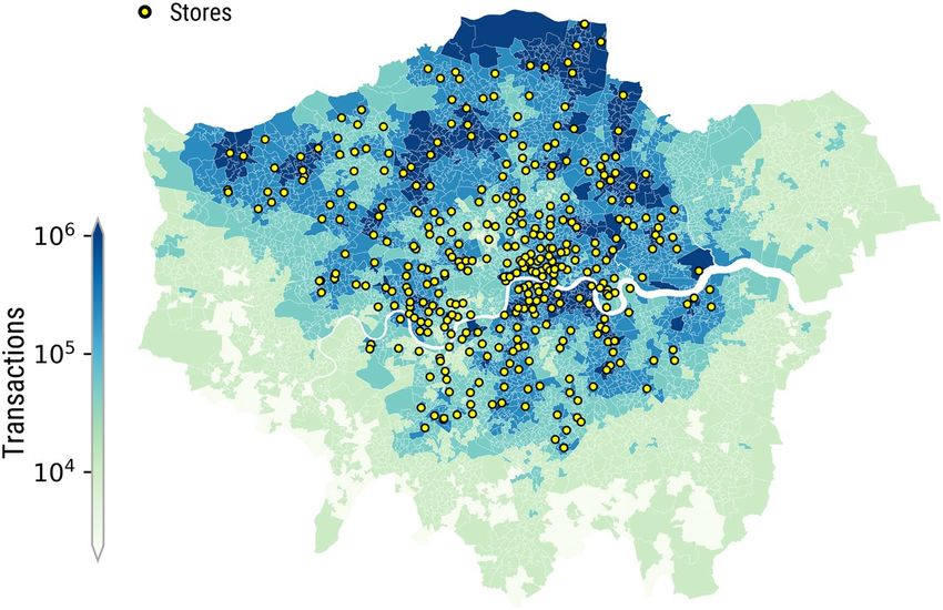
Coverage. As we will show in the Technical Validation section, the concentration of Tesco stores is higher in the
northern part of London. As a result, some areas of the city exhibit low penetration. In the dataset, we provide the
information to identify low-coverage areas and filter them out if needed.
Limited scope. The number of purchases considered is very large but by no means covers the full scope of food
consumption habits of London residents. Naturally, this dataset does not reflect food consumption in restaurants.
Also, it does not cover the grocery store purchases done in other chains or stores and, even among the Tesco
customers, it does not include information of online purchases and of products purchased by people who do not
own a Clubcard. In short, albeit this dataset reveals trends in food consumption habits at area level, it does not
represent the full picture of daily food consumption.
Average product. From our data, there is no way of estimating what is the diet of individual customers.
Therefore, the nutrient values are provided as averages over all the items purchased by the residents of an area.
In other words, we represent the nutritional features of the hypothetical average product consumed in the area.
This type of representation is appropriate for some types of analysis but introduces limitations to any study that
requires an average representation at the level of individuals, rather than at the level of geographical area.
Data Records
We made the dataset available through Figshare45 under the Creative Commons International license 4.0 (CC
BY 4.0).
Food items and their categories. We provide the list of products contained in each food category. The
identifiers associated with products can be used to query external services to get additional information about
them. This information is stored in a single .csv file named food_categories.csv.
• GTIN Global Trade Item Number, a standard identifier for trade items developed by GS1, a not-for-profit
organization that develops and maintains global standards for business communication. Specifically, the
GTIN is the number that comes with the barcode on the product label. GS1 offers an online service for GTIN
lookup (http://gepir.gs1.org/index.php/search-by-gtin).
• Category. The product category. The possible categories are: beer, dairy, eggs, fats & oils, fish, fruit & veg,
grains, red meat, poultry, readymade, sauces, soft drinks, spirits, sweets, tea & coffee, water, and wine.
Area descriptors. For each geographic aggregation (LSOA, MSOA, Ward, Borough) we provide a.csv file
({aggregation}_grocery.csv) containing the aggregated information on food purchases, enriched with informa-
tion coming from the census. We provide data for two temporal aggregations. One file summarizing the data for
the full year and 12 files with the data for each of the calendar months. Each file contains 202 columns. Below,
we provide a short description of all the fields. References to equations introduced in the Methods section are
reported when appropriate.
• area_id. Identifier of the area.
• weight. Weight of the average food product, in grams (Eq. (3))
• volume. Volume of the average drink product, in liters (Eq. (4))
• energy. Nutritional energy of the average product, in kcals (Eq. (5))
• energy_density. Concentration of calories in the area’s average product, in kcals/gram (Eq. (6))
• {nutrient}. Weight of {nutrient} in the average product, in grams (Eq. (7)). Possible nutrients are: carbs, sugar,
fat, saturated fat, protein, fibre. The count of carbs include sugars and the count of fats includes saturated fats.
• energy_{nutrient}. Amount of energy from {nutrient} in the average product, in kcals (Eq. (8))
• h_nutrients_weight. Entropy of nutrients weight (Eq. (11))
Scientific Data | (2020) 7:57 | https://doi.org/10.1038/s41597-020-0397-7 5www.nature.com/scientificdata/ www.nature.com/scientificdata
Fig. 2 Distribution of residents and customers. Probability density function (pdf) of the number of residents
across LSOAs (left), and that of the number of customers (right).
• h_nutrients_weight_norm. Entropy of nutrients weight, normalized in [0,1].
• h_nutrients_calories. Entropy of energy from nutrients (Eq. (12))
• h_nutrients_calories_norm. Entropy of energy from nutrients, normalized in [0,1].
• f_{category}. Fraction of products of type {product_type} purchased (Eq. (13)).
• f_{category}_weight. Fraction of total product weight given by products of type {category} (Eq. (15)).
• h_category. Entropy of food product types (Eq. (14)).
• h_category_norm. Entropy of food product categories, normalized in [0,1].
• h_category_weight. Entropy of weight of food product categories (Eq. (16)).
• h_category_weight_norm. Entropy of weight of food product categories, normalized in [0,1].
• representativeness_norm. The ratio between the number of unique customers in the area and the number of
residents as measured by the census; values are min-max normalized in [0,1] across all areas (Eq. (2)).
• transaction_days. Number of unique dates in which at least one purchase has been made by one of the resi-
dents in the area.
• num_transactions. Total number of products purchased by Clubcard owners who are resident in the area.
• man_day. Cumulative number of man-days of purchase (number of distinct days a customer has purchased
something, summed all individual customers).
• population. Total population of residents in the area according to the 2015 census.
• male. Total male population in the area.
• female. Total female population in the area.
• age_0_17. Total number of residents between 0 and 17 years old.
• age_18_64. Total number of residents between 18 and 64 years old.
• age_65 + . Total number of residents aged 65 years or more.
• avg_age. Average age of residents according to the 2015 census.
• area_sq_km. Surface of the area (km2).
• people_per_sq_km. Population density per km2.
Where applicable, measures are accompanied with their standard deviation (fields with suffix _std), the 95%
confidence interval for the mean (suffix _ci95), and the values of the 2.5th, 25th, 50th, 75th, and 97.5th percentiles
(suffix _perc{value}).
Technical Validation
This dataset is reliable when considering a variety of aspects: it reliably records all the purchases made at the
supermarket tills when using fidelity cards; reports the nutritional information of individual products as accu-
rately as the labels of the original products do; and comes with verified customer locations (they are the areas to
which the fidelity cards were sent to). Yet, there are two aspects that need validation: i) the representativeness
of the Tesco customer base; and ii) the ecological validity of the aggregated grocery data, namely how well they
represent the general patterns of food consumption at area-level, which we estimate through food-related health
outcomes in those areas.
Validation of area representativeness. In each LSOA, we consider two quantities: number of cus-
tomers and number of residents. Their frequency distributions differ (Fig. 2): that of the number of residents
is bell-shaped (as LSOAs have been designed to partition a city in patches containing a comparable number of
residents), while that of the number of customers is skewed (not least because, as Fig. 3 shows, Tesco stores are
not uniformly distributed across the city). Therefore, not only penetration rates of stores are distributed unevenly
across the city, but also those of purchases are. As a result, in certain areas, the customers are not representative
of the general population.
To fine-tune the desired level of general population’s representativeness, researchers can consider not all areas
but only part of them. To allow them to do so, we report each area’s representa tiveness(a) (the ratio between the
number of customers and the number of residents). The higher it is, the more representative that area’s data is of
the general population. We find that, if one considers only the areas with at least 0.1 representativeness (x-axis
in Fig. 4 (left)), one is left with 80% of the total number of areas (x-axis). That is, at least 10% of the residents are
Scientific Data | (2020) 7:57 | https://doi.org/10.1038/s41597-020-0397-7 6www.nature.com/scientificdata/ www.nature.com/scientificdata
Fig. 3 London map reflecting the stores’ positions (dots) and the number of grocery transactions at LSOA level
(the darker the color, the higher the number of transactions).
Fig. 4 Data representativeness. Left: The percentage of areas (y-axis) that have a level of representativenessnorm
at least thresholdr (x-axis). Right: The Spearman rank correlation between the number of customers and
the number of residents with a given %considered areas (x-axis) (areas are ordered by decreasing levels of
representativeness). Results are presented for three different geographic aggregations (LSOA, MSOA, and
Wards). Correlations are all statistically significant with p < 0.01.
customers in each area. This is a conservative estimate as it assumes that each fidelity card is used to purchase food
for one single person, while it might well be used to satisfy the needs of an entire family.
Then, if one were to take that top 80% of the areas ranked by representativeness, the overall correlation
between the number of customers and the number of residents would be considerable: it goes from 0.38 for
LSOAs to 0.58 for wards (Fig. 4 (right)). If one were to take only the 10% most representative areas instead, then
that correlation would be as high as 0.75 for LSOAs to 0.84 for wards (Fig. 4 (right)).
More generally, the larger the set of considered areas, the lower that correlation: depending on their needs,
researchers have to balance the number of total areas they wish to consider, and the correlation between the
number of customers and that or residents they wish to obtain. For example, considering 80% of the areas yields
correlations between 0.38 (LSOAs) and 0.58 (wards).
Validation of health outcomes. We assess the ecological validity of the data by comparing the grocery
purchases with metabolic syndrome conditions that are strongly linked to food consumption habits. Specifically,
we consider data about the prevalence of obesity and type-2 diabetes.
• Prevalence of overweight and obese children. The fractions of overweight and obese primary school chil-
dren in Reception class (aged 4 to 5) and year 6 (aged 10 to 11), sampled across wards. This data has been
collected by the English National Health Service (NHS) in the 2013–2014 school year46.
Scientific Data | (2020) 7:57 | https://doi.org/10.1038/s41597-020-0397-7 7www.nature.com/scientificdata/ www.nature.com/scientificdata
Fig. 5 Spearman rank correlation between prevalence of metabolic syndrome conditions and food
consumption estimators: energy (energy(a), Eq. (5)); entropy of nutrients (Henergy-nutrients(a), Eq. (12)); and energy
from individual nutrients (energy-nutrienti(a), Eq. (8)). Only statistically significant correlations (p < 0.05) are
shown.
• Prevalence of overweight and obese adults. The fractions of overweight and obese individuals among a sta-
tistical sample of borough residents. This data has been collected by the Active People Survey (APS) in 201247.
• Diabetes prevalence. The fraction of adults among those registered at a GP practice in England who are
affected by type-2 diabetes48. This data has been collected by the NHS for year 2015 at ward level.
Nutrients and metabolic syndrome. According to the World Health Organization49, the three best die-
tary habits to prevent conditions associated with the metabolic syndrome are: i) limiting the intake of calories;
ii) having a nutrient-diverse diet; and iii) favoring the consumption of fibers and proteins over sugars, carbohy-
drates, and fat. To verify whether the violation of these three recommendations is associated with an increased
prevalence of metabolic disorders, we correlate diabetes and obesity prevalence with: i) the energy of the typical
product (energy(a), Eq. (5)); ii) the entropy of energy intake from different nutrients (Henergy-nutrients(a), Eq. (12));
iii) and the energy content of each individual nutrient (energy-nutrienti(a) Eq. (8)).
Spearman rank correlations (R) between nutrients and prevalence of medical conditions across areas are sum-
marized in Fig. 5.
The prevalence of obese and overweight children (Fig. 5, top row) is inversely correlated with the energy com-
ing from fibers in the typical product, with correlations all lower than −0.5. We found a weaker inverse correla-
tion (R ≅ − 0.2) with energy coming from proteins and with the entropy of nutrients and, only for children in
reception year, with saturated fats (R ∈ [ −0.1, − 0.15]). We found a positive yet feeble association (R ≅ 0.1) with
energy from carbohydrates.
Stronger correlations emerge for adults (Fig. 5, bottom row). Areas with higher prevalence of overweight and
obese adults are those where the typical product is higher in energy (R ≅ 0.4) and is also high in fat, sugar, and
carbohydrates (R ∈ [0.35, 0.45]). Prevalence of adult obesity is negatively associated with nutrient entropy
(R ≅ − 0.4). The diabetes data yields the highest number of significant correlations (Fig. 5, bottom-right panel).
High diabetes prevalence is found in areas where the food purchased is higher in energy coming from carbohy-
drates, sugar, and to a lesser extent fats (R ∈ [0.35, 0.65]). Low diabetes prevalence is associated with high con-
sumption of fibers and proteins (R ≅ 0.5), especially in areas characterized by high entropy of nutrients
(R = − 0.77).
To build stronger evidence that the food descriptors provided in the dataset are directly linked to food-related
illnesses–and not just proxies for confounding determinants of those ailments–we ran an ordinary least squares
regression. The regression aims at predicting the prevalence of diabetes from the two highest-correlated factors
(energy-carbs and Henergy-nutrients) and four control variables accounting for demographics and store penetration
rates: average age, % of female residents, density of residents in the area, and number of transactions. Where
necessary, predictor variables undergo a logarithmic transformation. We also applied a min-max rescaling of
Scientific Data | (2020) 7:57 | https://doi.org/10.1038/s41597-020-0397-7 8www.nature.com/scientificdata/ www.nature.com/scientificdata
Diabetes
Feature Coefficient Std. error p
α (intercept) 0.9362 0.081
energy-carbs 0.1883 0.065 0.000
Henergy-nutrients −1.0252 0.084 0.004
Average age −0.1191 0.041 0.000
% Females −0.1237 0.049 0.004
Transactions 0.2853 0.035 0.012
Pop. density −0.0767 0.034 0.000
Durbin-Watson stat. = 1.265 Adj R2 = 0.613
Table 2. Linear regression to predict ward diabetes prevalence from carbohydrates (energy-carbs), nutrient
entropy (Henergy-nutrients), and control variables.
Fig. 6 Diabetes prevalence estimates. Actual ward diabetes prevalence values at Ward level vs. values estimated
by a linear regression with carbohydrates and nutrient entropy as the only two independent variables (left).
Average standardized regression residuals for areas with varying values of representativeness (right). 95%
confidence intervals are shown.
each variable, which allowed us to compare the relative importance of different factors in predicting the out-
come. Results are summarized in Table 2. The model has a high goodness of fit (R2 > 0.6) especially compared
to a baseline model where only the control variables are considered (R2 = 0.14). The magnitude of the regression
coefficients indicates that all independent variables have predictive power, with the nutrient entropy being the
strongest one.
A regression model that includes only energy-carbs and Henergy-nutrients as independent variables retains a high
explanatory power (R2 = 0.56). We plotted the actual diabetes prevalence values against the values predicted by
this 2-variable regression model in Fig. 6 (left). We checked how the standardized regression residuals–namely
the absolute differences between the official diabetes estimates and the corresponding predicted values, divided by
the standard deviation of all residuals–vary with area a’s representa tiveness(a) (the ratio between the number of
customers and the number of residents). To do that, we partition areas in equally-sized groups of areas with com-
parable values of representativeness, and average the standardized residuals within each group (Fig. 6 (right)).
The prediction error is higher for areas in which the representativeness is lower (www.nature.com/scientificdata/ www.nature.com/scientificdata
Usage Notes
Data parsing. All files are provided in comma separated value format, with header on the first line and one
record per line. This type of files is easily parsed with any programming language (e.g., R, Python) or spreadsheet
utilities (e.g., OpenOffice Calc).
Spatial definition. The spatial data ({aggregation}_grocery_info.csv files) can be integrated with other data-
sets using the geographical area identifier–the first column in every file–as join key. It is important to note that
the boundaries of the geographical areas were periodically redefined in the past decades. In the dataset, we use
the 2011 definition of LSOAs, MSOAs and Boroughs (the most recent one at the time of writing) and the 2015
definition of wards. The list of area ids over time and instructions on how to map data across aggregation levels
are available on the official London Greater Authority atlas43.
Area filtering. In the Technical Validation Section, we showed that filtering out areas with lower coverage
yields a sample that is more representative of the general population. The same type of filtering can be achieved by
retaining only the entries with highest values of representativeness.
Code availability
We provide the code we used to validate our data in the form of a python script.
Received: 8 July 2019; Accepted: 29 January 2020;
Published: xx xx xxxx
References
1. Deloitte. Global powers of retailing 2017 - the art and science of customers. https://www2.deloitte.com/content/dam/Deloitte/
global/Documents/consumer-industrial-products/gx-cip-2017-global-powers-of-retailing.pdf (2017).
2. Kantar. Worldpanel grocery share data. https://uk.kantar.com/consumer/shoppers/2015/march-kantar-worldpanel-uk-grocery-
share/ (2015).
3. Ahn, Y.-Y., Ahnert, S. E., Bagrow, J. P. & Barabási, A.-L. Flavor network and the principles of food pairing. Scientific reports 1 (2011).
4. Zagheni, E., Garimella, V. R. K., Weber, I. & State, B. Inferring international and internal migration patterns from twitter data. In
Proceedings of the 23rd International Conference on World Wide Web, WWW ’14 Companion, 439–444 (2014).
5. Kershen, A. J. Food in the migrant experience (Routledge, 2017).
6. Hughes, K. et al. Young people, alcohol, and designer drinks: quantitative and qualitative study. BMJ 314, 414 (1997).
7. Cummins, S. & Macintyre, S. “food deserts”: Evidence and assumption in health policy making. BMJ 325, 436 (2002).
8. James, W. P. T., Nelson, M., Ralph, A. & Leather, S. Socioeconomic determinants of health: the contribution of nutrition to
inequalities in health. BMJ 314, 1545 (1997).
9. Curtis, H. J. & Goldacre, B. Openprescribing: normalised data and software tool to research trends in English NHS primary care
prescribing 1998–2016. BMJ open 8, e019921 (2018).
10. Blaxter, M. Health and lifestyles (Routledge, 2003).
11. Williams, P. Consumer understanding and use of health claims for foods. Nutrition reviews 63, 256–264 (2005).
12. Abbar, S., Mejova, Y. & Weber, I. You tweet what you eat: Studying food consumption through twitter. In Proceedings of the 33rd
Annual ACM Conference on Human Factors in Computing Systems, CHI ’15, 3197–3206 (2015).
13. Kagaya, H. & Aizawa, K. Highly accurate food/non-food image classification based on a deep convolutional neural network. In
International Conference on Image Analysis and Processing, 350–357 (Springer, 2015).
14. Lawrence, R. D., Almasi, G. S., Kotlyar, V., Viveros, M. & Duri, S. S. Personalization of supermarket product recommendations. In
Applications of Data Mining to Electronic Commerce, 11–32 (Springer, 2001).
15. Sano, N., Machino, N., Yada, K. & Suzuki, T. Recommendation system for grocery store considering data sparsity. Procedia Computer
Science 60, 1406–1413 (2015).
16. Guidotti, R., Rossetti, G., Pappalardo, L., Giannotti, F. & Pedreschi, D. Personalized market basket prediction with temporal
annotated recurring sequences. IEEE Transactions on Knowledge and Data Engineering (2018).
17. Prasad, A., Strijnev, A. & Zhang, Q. What can grocery basket data tell us about health consciousness? International Journal of
Research in Marketing 25, 301–309 (2008).
18. Howard, S., Adams, J. & White, M. Nutritional content of supermarket ready meals and recipes by television chefs in the united
kingdom: cross sectional study. BMJ e7607 (2012).
19. Instacart. The instacart online grocery shopping dataset. https://www.instacart.com/datasets/grocery-shopping-2017 (2017).
20. West, R., White, R. W. & Horvitz, E. From cookies to cooks: Insights on dietary patterns via analysis of web usage logs. In Proceedings
of the 22Nd International Conference on World Wide Web, WWW’13, 1399–1410 (2013).
21. Wagner, C., Singer, P. & Strohmaier, M. The nature and evolution of online food preferences. EPJ Data. Science 3, 38 (2014).
22. Sajadmanesh, S. et al. Kissing cuisines: Exploring worldwide culinary habits on the web. In Proceedings of the 26th International
Conference on World Wide Web Companion, WWW ’17 Companion, 1013–1021 (2017).
23. Trattner, C. & Elsweiler, D. Food recommender systems: important contributions, challenges and future research directions. arXiv
preprint arXiv:1711.02760 (2017).
24. Kusmierczyk, T., Trattner, C. & Nørvåg, K. Understanding and predicting online food recipe production patterns. In Proceedings of
the 27th ACM Conference on Hypertext and Social Media, 243–248 (ACM, 2016).
25. Asano, Y. M. & Biermann, G. Rising adoption and retention of meat-free diets in online recipe data. Nature Sustainability 2, 621–627
(2019).
26. Said, A. & Bellogín, A. You are what you eat! tracking health through recipe interactions. In Rsweb workshop at ACM Recsys (2014).
27. Trattner, C. & Elsweiler, D. Investigating the healthiness of internetsourced recipes: Implications for meal planning and
recommender systems. In Proceedings of the 26th International Conference on World Wide Web, WWW ’17, 489–498 (2017).
28. Ge, M., Ricci, F. & Massimo, D. Health-aware food recommender system. In Proceedings of the 9th ACM Conference on Recommender
Systems, RecSys ’15, 333–334 (2015).
29. Elsweiler, D., Trattner, C. & Harvey, M. Exploiting food choice biases for healthier recipe recommendation. In Proceedings of the 40th
International ACM SIGIR Conference on Research and Development in Information Retrieval, SIGIR ’17, 575–584 (2017).
30. Trattner, C., Parra, D. & Elsweiler, D. Monitoring obesity prevalence in the united states through bookmarking activities in online
food portals. PloS one 12, e0179144 (2017).
31. Mejova, Y., Haddadi, H., Noulas, A. & Weber, I. #foodporn: Obesity patterns in culinary interactions. In Proceedings of the 5th
International Conference on Digital Health 2015, DH ’15, 51–58 (2015).
32. Marin, J. et al. Recipe1m+: A dataset for learning cross-modal embeddings for cooking recipes and food images. IEEE Transactions
on Pattern Analysis and Machine intelligence (2019).
Scientific Data | (2020) 7:57 | https://doi.org/10.1038/s41597-020-0397-7 10www.nature.com/scientificdata/ www.nature.com/scientificdata
33. Ofli, F., Aytar, Y., Weber, I., al Hammouri, R. & Torralba, A. Is saki #delicious?: The food perception gap on instagram and its relation
to health. In Proceedings of the 26th International Conference on World Wide Web, WWW ’17, 509–518 (2017).
34. Chen, J. & Ngo, C.-W. Deep-based ingredient recognition for cooking recipe retrieval. In Proceedings of the 24th ACM international
conference on Multimedia, 32–41 (ACM, 2016).
35. Sharma, S. S. & De Choudhury, M. Measuring and characterizing nutritional information of food and ingestion content in
instagram. In Proceedings of the 24th International Conference on World Wide Web, WWW ’15 Companion, 115–116 (2015).
36. De Choudhury, M., Sharma, S. & Kiciman, E. Characterizing dietary choices, nutrition, and language in food deserts via social
media. In Proceedings of the 19th ACM Conference on Computer-Supported Cooperative Work & Social Computing, CSCW ’16,
1157–1170 (2016).
37. Mejova, Y., Abbar, S. & Haddadi, H. Fetishizing food in digital age:# foodporn around the world. In Proceedings of the 10th
International AAAIConference on Web and Social Media, ICWSM, 250–258 (AAAI, 2016).
38. Wagner, C. & Aiello, L. M. Men eat on mars, women on venus?: An empirical study of food-images. In Proceedings of the ACM Web
Science Conference, WebSci ’15, 63:1–63:3 (2015).
39. Aiello, L. M., Schifanella, R., Quercia, D. & Del Prete, L. Large-scale and high-resolution analysis of food purchases and health
outcomes. EPJ Data Science 8, 14 (2019).
40. Department of Health - Population Health Division. Technical guidance on nutrition labelling. https://assets.publishing.service.gov.
uk/government/uploads/system/uploads/attachment_data/file/595961/Nutrition_Technical_Guidance.pdf (2016).
41. European Council. 90/496/eec of 24 september 1990 on nutrition labeling for foodstuffs. Official Journal of the European Union 276,
40–44 (1990).
42. Whitney, E. & Rolfes, S. R. Understanding nutrition (Cengage Learning, 2007).
43. Greater London Authority. LSOA atlas. https://data.london.gov.uk/dataset/lsoa-atlas (2014).
44. Office for National Statistics. Lower layer super output area population estimates (supporting information). https://www.ons.gov.uk/
peoplepopulationandcommunity/populationandmigration/populationestimates/datasets/lowersuperoutputareamidyear-
populationestimates (2018).
45. Aiello, L. M., Schifanella, R., Quercia, D. & Del Prete, L. Tesco grocery 1.0. figshare. https://doi.org/10.6084/m9.figshare.c.4769354.
v2 (2020).
46. Department of Health. Prevalence of childhood obesity, borough, ward and msoa. https://data.london.gov.uk/dataset/prevalence-
childhood-obesity-borough (2014).
47. NHS Digital. Obesity in Adults. https://data.london.gov.uk/dataset/obesity-adults (2014).
48. NHS Digital. Quality and outcomes framework (QOF) - 2016-17. https://digital.nhs.uk/data-and-information/publications/
statistical/quality-and-outcomes-framework-achievement-prevalence-and-exceptions-data/quality-and-outcomes-framework-
qof-2016-17 (2017).
49. Amine, E. et al. Diet, nutrition and the prevention of chronic diseases: report of a Joint WHO/FAO Expert Consultation (World
Health Organization, 2002).
50. Patil, A., Huard, D. & Fonnesbeck, C. J. Pymc: Bayesian stochastic modeling in python. Journal of statistical software 35, 1 (2010).
51. Hoffman, M. D. & Gelman, A. The no-u-turn sampler: adaptively setting path lengths in hamiltonian monte carlo. Journal of
Machine Learning Research 15, 1593–1623 (2014).
52. Gelman, A., Goodrich, B., Gabry, J. & Vehtari, A. R-squared for bayesian regression models. The American Statistician 1–7 (2019).
Acknowledgements
We are grateful to Tesco for making the grocery purchase data available.
Author contributions
L.D.P. performed the data extraction and first-level spatial data aggregation. L.M.A., R.S. and D.Q. performed the
data augmentation and technical validation. All authors contributed to drafting the manuscript.
Competing interests
The authors declare no competing interests.
Additional information
Correspondence and requests for materials should be addressed to L.M.A.
Reprints and permissions information is available at www.nature.com/reprints.
Publisher’s note Springer Nature remains neutral with regard to jurisdictional claims in published maps and
institutional affiliations.
Open Access This article is licensed under a Creative Commons Attribution 4.0 International
License, which permits use, sharing, adaptation, distribution and reproduction in any medium or
format, as long as you give appropriate credit to the original author(s) and the source, provide a link to the Cre-
ative Commons license, and indicate if changes were made. The images or other third party material in this
article are included in the article’s Creative Commons license, unless indicated otherwise in a credit line to the
material. If material is not included in the article’s Creative Commons license and your intended use is not per-
mitted by statutory regulation or exceeds the permitted use, you will need to obtain permission directly from the
copyright holder. To view a copy of this license, visit http://creativecommons.org/licenses/by/4.0/.
The Creative Commons Public Domain Dedication waiver http://creativecommons.org/publicdomain/zero/1.0/
applies to the metadata files associated with this article.
© The Author(s) 2020
Scientific Data | (2020) 7:57 | https://doi.org/10.1038/s41597-020-0397-7 11You can also read