Large Scale Cohesive Subgraphs Discovery for Social Network Visual Analysis
←
→
Page content transcription
If your browser does not render page correctly, please read the page content below
Large Scale Cohesive Subgraphs Discovery for Social
                     Network Visual Analysis

                                     Feng Zhao                                                          Anthony K. H. Tung
                            School of Computing                                                        School of Computing
                       National University of Singapore                                           National University of Singapore
                     zhaofeng@comp.nus.edu.sg                                                       atung@comp.nus.edu.sg

ABSTRACT                                                                                     Cohesive subgraph discovery is an intriguing problem and
Graphs are widely used in large scale social network analy-                               has been widely studied for decades. One fundamental struc-
sis nowadays. Not only analysts need to focus on cohesive                                 ture is the clique in which every pair of vertices is connected.
subgraphs to study patterns among social actors, but also                                 Finding cliques is NP-Hard [9] and many work try to re-
normal users are interested in discovering what happening in                              lax the clique problem to improve efficiency [15, 1, 19, 18,
their neighborhood. However, effectively storing large scale                              24, 22]. However, these methods do not directly take the
social network and efficiently identifying cohesive subgraphs                             characteristics of social network into consideration. For ex-
is challenging. In this work we introduce a novel subgraph                                ample, in Figure 1a, we emphasize the 3-core in solid edges
concept to capture the cohesion in social interactions, and                               and connected vertices, in which every vertex v inside it
propose an I/O efficient approach to discover cohesive sub-                               satisfies d(v) ≥ 3. However, g is not cohesive enough as a
graphs.                                                                                   whole. Considering cliques inside g, we can find a 5-clique
   Besides, we propose an analytic system which allows users                              (a, b, c, d, f ) and a 4-clique (c, d, e, f ) on the left, as well as
to perform intuitive, visual browsing on large scale social                               two 4-cliques {(m, n, p, q), (p, q, t, u)} on the right. But ver-
networks. Our system stores the network as a social graph                                 tex a and p are not tightly coupled since they only share one
in the graph database, retrieves a local cohesive subgraph                                common neighbor j, so the subgraph g is better viewed as
based on the input keywords, and then hierarchically visu-                                two separated cohesive groups.
alizes the subgraph out on orbital layout, in which more                                     This phenomenon, denoted as the tie strength concept, is
important social actors are located in the center. By sum-                                well studied in the sociological area. Note that tie is same as
marizing textual interactions between social actors as tag                                edge in social graph. Mark Granovetter in his landmark pa-
cloud, we provide a way to quickly locate active social com-                              per [14] indicates that two actors A and B are likely to have
munities and their interactions in a unified view.                                        many friends in common if they have a strong tie. In another
                                                                                          state-of-the-art sociological paper, White et al. [25] observe
                                                                                          that a group is cohesive to the extent that pairs of its mem-
1.     INTRODUCTION                                                                       bers have multiple social connections, direct or indirect, but
                                                                                          within the group, that pull it together. One intuitive real life
   Graphs play a seminal role in social network analysis nowa-
                                                                                          example is that you and your intimate friends in Facebook
days. A large and rapidly growing social network companies
                                                                                          may have high possibility to share lots of mutual friends.
store social data as graph structures, such as Facebook1 and
                                                                                          However, this observation has been missing from many of
Twitter2 . In a social graph, vertices represent social ac-
                                                                                          the cohesive subgraph definitions, which drives us to define
tors, while edges represent relationships or interactions be-
                                                                                          a “mutual-friend” structure to capture the tie strength in
tween actors. One fundamental operation on social graph
                                                                                          a quantitative manner for social network analysis. Assume
is to identify groups of social actors that are highly con-
                                                                                          we consider a tie in Figure 1 valid if and only if it is sup-
nected with each other, represented by a cohesive subgraph,
                                                                                          ported by at least two mutual friends. With only supported
in which analysts may discover interesting structural pat-
                                                                                          by one mutual friend j, the tie (a, p) should be disconnected
terns among social actors, and normal users can know what
                                                                                          according to the mutual-friend concept, and we successfully
happening in their neighborhood.
                                                                                          separate subgraph g to two groups. We will formally define
                                                                                          the problem and compare it to other definitions in details in
1
    https://www.facebook.com                                                              the subsequent sections.
2
    https://www.twitter.com                                                                  How to improve the scalability is one potential challenge
                                                                                          of cohesive subgraph discovery for social network analysis.
Permission to make digital or hard copies of all or part of this work for
                                                                                          Most of the existing approaches [23, 24, 26] mainly focus
personal or classroom use is granted without fee provided that copies are                 on the dense region recognition for moderate size graphs.
not made or distributed for profit or commercial advantage and that copies                However, many practical social network applications need to
bear this notice and the full citation on the first page. To copy otherwise, to           store the large scale graph in disks or databases. Like Face-
republish, to post on servers or to redistribute to lists, requires prior specific        book, over 800 million active actors use its service per month
permission and/or a fee. Articles from this volume were invited to present                all over the world [3], which is impossible to fit in memory.
their results at The 39th International Conference on Very Large Data Bases,
August 26th - 30th 2013, Riva del Garda, Trento, Italy.
                                                                                          Therefore, besides providing memory based solutions, we fo-
Proceedings of the VLDB Endowment, Vol. 6, No. 2                                          cus on developing a solution to handling large scale social
Copyright 2012 VLDB Endowment 2150-8097/12/12... $ 10.00.

                                                                                     85
• We have introduced a novel cohesive subgraph con-
cept to capture the intrinsic feature of social network
analysis nicely.
• By leveraging graph databases, we have devised an of-
fline algorithm to compute global cohesive subgraphs
efficiently. Moreover, we have developed an online
algorithm to further refine local cohesive subgraphs
(a) Before Layout based on the results of offline computations.
• We have developed an orbital layout to decompose the
cohesive subgraph into a set of orbits, and coupled
with tag cloud summarization, which allows users to
locate important actors and their interactions inside
subgraphs clearly.
• We have conducted extensive experiments, and the re-
sults show that our approach is both effective and ef-
ficient.
The rest of the paper is organized as follows. Section 2
reviews the related literature on cohesive subgraph finding
(b) After Layout and social network analysis. Section 3 defines the cohe-
sive subgraph discovery problem handled throughout this
Figure 1: Cohesive Graph Example paper. Section 4 presents the offline computations in the
graph database, and the online visual analytic system is de-
scribed in Section 5. Our extensive experimental study is
reported in Section 6. Section 7 concludes the paper.
graphs stored in a graph database, which is more scalable
for graph operations than a relational database. Like Twit-
ter, recently it migrated its social graph to FlockDB [10], 2. RELATED WORK
a distributed, fault-tolerant graph database for managing Modeling a cohesive subgraph mathematically has been
data at webscale. By leveraging graph databases, we extend extensively studied for decades. One of the earliest graph
memory based algorithms to I/O efficient solutions for large models was the clique model [16], in which there exists an
scale social networks. edge between any two vertices. However, the clique model
Additionally, exploring and analyzing social network can idealizes cohesive properties so that it seldom exists and
be time consuming and not user-friendly. Visual represen- hard to compute. Alternative approaches are suggested that
tation of social networks is important for understanding the essentially relaxes the clique definition in different aspects.
network data and conveying the result of the analysis. How- Luce [15] introduces a distance based model called k-clique
ever, it is a challenge to summarize the structural patterns and Alba [1] introduces a diameter based model called k-
as well as the content information to help users analyze the club. Generally speaking, these models relax the reacha-
social network. One previous work [23] proposes a novel bility among vertices from 1 to k. Another line of work
linear plot for graph structure, which sketches out the dis- focuses on a degree based model, like k-plex [19] and k-
tribution of dense regions and is suitable for static dense core [18]. The k-plex is still NP-Complete since it restricts
pattern discovery. Unlike this work, our system insulates the subgraph size, while k-core further relaxes it to achieve
users from the complexities of social analysis by visualiz- the linear time complexity with respect to the number of
ing cohesive subgraphs and the contents in an interactive edges. A new direction based on the edge triangle model,
fashion. For graph structure, we propose an orbital layout like DN-Graph [24] and truss decomposition [22], is more
to decompose the graph into hierarchy with respect to the suitable for social network analysis since it captures the tie
cohesive value, in which more important social actors are strength between actors inside the subgroup. Our proposed
located in the center. Figure 1b shows an orbital layout for mutual friend concept belongs to this model and we will
the graph in Figure 1a. Briefly speaking, this layout consists compare it with the above two concepts in Section 3 in de-
of four orbits with four different colors, in which the more tails. Recently, database researchers try to scale up the disk
cohesive vertices are located closer to the center. Like the based cohesive subgraph discovery. Cheng et al. [6] pro-
5-clique (a, b, c, d, f ), all five vertices are in the innermost or- pose a partition based solution for massive k-core mining.
bit. As for vertices size setting, ordering and edge filtering, They also develop a disk based triangulation method [7] as a
we will explain them in details later in this paper. For the fundamental operation for cohesive subgraph discovery. Dif-
contents, we make use of tag cloud technique to summarize ferently, we store the social graph in graph database that is
the major semantics for a group of social actors. Gener- more scalable for graph traversal based algorithms.
ally speaking, our visualization is flexible and can be easily Besides, social network characteristics has been well in-
applied to other cohesive graph concepts. vestigated in sociology communities. The most related one
In this paper, we develop a novel social network visual is the tie strength theory, which is introduced by Mark Gra-
analytic framework for large scale cohesive subgraphs dis- novetter in his landmark paper [14]. Recently, many so-
covery. Our contributions are summarized as follows: cial network researchers investigate this important theory
86in online social network, such as the user behaviors in Face- 3.2 The k -mutual-friend Subgraph
book [12, 3] and Twitter [13]. Their conclusions show that
the strength of tie is still a tenable theory in social media, Definition 3.2. (k-mutual-friend Subgraph)
which are the bases of the mutual-friend subgraph definition A k-mutual-friend is a connected subgraph g ∈ G such that
in this paper. each edge is supported by at least k pairs of edges forming a
Social network visualization and analysis has received a triangle with that edge within g. The k-mutual-friend num-
great deal of attention recently. Wang et al. [23] proposes ber of this subgraph, denoted as M(g), equals k.
a linear plot based on graph traversal to capture the dense
subgraph distribution in the whole graph. Zhang et al. [26] Note that we need to exclude the trivial situation to con-
extends it to compare the pattern changing between two sider a single vertex as a mutual-friend. Given the parameter
graph snapshots. Place vertices in concentric circles with k, we may discovery many k-mutual-friend subgraphs that
different levels is a popular way to visualize graph struc- overlap with each other. In the worst case, the number of
tures, such as k shell decomposition [2], centralities visu- k-mutual-friend subgraphs can be exponential to the graph
alization [8] and so on. We leverage the circular idea and size. Therefore, we further define the maximal k -mutual-
devise the orbital layout to visualize k-mutual-friend sub- friend subgraph to avoid redundancy.
graphs in an interactive manner. Note that the orbital lay-
out is perpendicular to linear plot. We could seamlessly in- Definition 3.3. (Maximal k-mutual-friend Subgraph)
tegrate the linear plot for global subgraph distribution and A maximal k-mutual-friend subgraph is a k-mutual-friend
the orbital layout for local subgraph representation. Besides, subgraph that is not a proper subgraph of any other k-mutual-
friend subgraph.
Arnetminer [21] provides comprehensive search and mining
services for academic social networks. It is a full fledged To compare with clique and core, we present two interest-
framework with nice visual exploring function like the rela- ing properties about the k -mutual-friend subgraph.
tionship graph between two researchers. However, the focus
of this visualization is to show the connections between two Property 3.1. Every (k + 2)-clique of G is contained in a
researchers instead of the importance of individuals in the k-mutual-friend of G.
cohesive subgraphs as in our solution.
Proof. Since a (k + 2)-clique is a fully connected sub-
graph with order k + 2, each edge is supported by k triangles.
3. PROBLEM DEFINITION Therefore, it is contained in a k-mutual-friend subgraph by
In this section, we first introduce the preliminary knowl- Definition 3.2.
edge, then define the maximal k-mutual-friend finding prob-
lem, and show several important properties about this con- Property 3.2. Every k-mutual-friend of G is a subgraph
cept. Furthermore, we compare it with clique, k-core, DN - of a (k + 1)-core of G.
Graph as well as truss decomposition in depth. Proof. For each vertex v in gk , it connects to at least
k triangles. Every triangle adds one neighbor vertex to v
3.1 Preliminaries except the first adding two neighbors, so that v has (k + 1)
As stated in Section 1, we model a social network as an neighbors, i.e. d(v) ≥ (k + 1). Therefore, gk qualifies as a
undirected, simple social graph G(V, E) in which vertices (k + 1)-core of G.
represent social actors and edges represent interactions be-
tween actors. The k-mutual-friend subgraph proposed in The above two properties suggest one important observa-
this paper is derived from clique and k -core [18]. Clique is a tion: (k + 2)-clique ⊆ k-mutual-friend ⊆ (k + 1)-core, show-
fully connected subgraph, in which every pair of vertices is ing that the mutual-friend is a kind of cohesive subgraph
connected by an edge. If the size of a clique is c, we call the between the clique and the core. Note that the reverse
clique a c-clique. k -core is one successful degree relaxation of the above two properties are not true. Again in Fig-
of clique concept defined as follows. ure 1, the 4-clique (m, n, p, q) is a subgraph of the 2-mutual-
friend (m, n, p, q, t, u), while 2-mutual-friend (a, b, c, d, e, f )
Definition 3.1. (k-core Subgraph) and (m, n, p, q, t, u), both of them are contained in the 3-core
A k-core is a connected subgraph g such that each vertex v (a, b, c, d, e, f, m, n, p, q, t, u). Finally, we define the main
has degree d(v) ≥ k within the subgraph g. problem we investigate in this paper as follows.
The k-core is motivated by the property that every vertex Problem 1. (Maximal k-mutual-friend Subgraph Finding)
has degree d(v) = c − 1 in a c-clique. k-core also needs to Given a social graph G(V, E) and the parameter k, find all
satisfy the degree condition, but the restriction on subgraph the maximal k-mutual-friend subgraphs.
size is not required. As such, k-core can be efficiently com-
puted in O(|E|) time complexity [18]. Differently, based on 3.2.1 Comparison to DN -Graph
the observation in Section 1, we propose the k-mutual-friend Before we illustrate the solution to Problem 1, we further
subgraph to emphasize on tie strength. One important prop- state an interesting connection between the mutual-friend
erty about edges in clique is that every edge is supported by concept and the DN -Graph concept proposed by Wang et
T r(e) = k − 2 triangles in a k-clique. Analogous to the k- al. [24] recently. A DN -Graph, denoted by G′ (V ′ , E ′ , λ),
core definition, the k -mutual-friend sets a lower bound for is a connected subgraph G′ (V ′ , E ′ ) of graph G(V, E) that
every edge’s triangle count. Next we will formally define the satisfies the following two conditions: (1) Every connected
k -mutual-friend and show its relationships to other cohesive pair of vertices in G′ sharesSat least λ common neighbors.
structures. (2) For any v ∈ V \V ′ , λ(V ′ {v}) < λ; and for any v ∈ V ′ ,
λ(V ′ − {v}) ≤ λ.
87At the first glance, DN -graph is similar to the maximal T r(e(d, f )) reduces to 3 but still satisfies the condition. Be-
k-mutual-friend subgraph. However, these two concepts are cause all the remaining edges with triangle counts larger than
distinct due to the second condition in DN -Graph defini- or equal to 2, the graph remains unchanged and the loop ter-
tion. Intuitively, the DN -graph defines a strict condition minates. Lastly, we delete all the isolated vertices and obtain
that the maximal subgraphs need to reach the local maxi- 2-mutual-friend (a, b, c, d, e, f ) as in Figure 2b.
mum even for adding or deleting only one vertex. On the
other hand, the maximal k-mutual-friend defines the local
maximal subgraph that is not a proper subgraph of any other
k -mutual-friend subgraph. As demonstrated in Figure 1a,
(m, n, p, q), (p, q, t, u) and (m, n, p, q, t, u) are all DN -Graphs
with λ = 2, since the λ value can only decrease if adding or
removing any vertices. However, only (m, n, p, q, t, u) is the
maximal 2-mutual-friend since other two are its subgraphs.
This example shows that the DN -Graph finding may gen-
erate many redundant subgraphs. Furthermore, due to the
hardness of satisfying the second condition, solving the DN -
Graph problem is NP-Complete as proven by the authors. (a) Step one (b) Step two
To solve it they iteratively refine the upper bound for each Figure 2: Example of in Memory Algorithm
edge to approach the real value, but it still has high com-
Although this is a straight forward solution, the compu-
plexity and isn’t suitable for large scale graph. Actually, the
tational complexity is relatively high because it has lots of
mutual friend finding is inspired by the DN -Graph concept
unnecessary triangle computations. In the worst case it re-
and we improve it by providing efficient solution in polyno-
moves one edge at a time and needs |E| times loops to re-
mial time subsequently.
move all the Pedges from G. As such, the total complex-
3.2.2 Comparison to Truss Decomposition ity is |E| × e(u,v)∈G (d(u) + d(v)), in which d(u) + d(v) is
the complexity to compute the triangle count for one edge.
Truss decomposition is a process to compute the k-truss of
This expression
P can be further simplified to the order of
a graph G for all 2 ≤ k ≤ kmax , in which k-truss is a cohesive
|E| × v∈G d(v)2 , because we need to get the v’s neigh-
subgraph ensures that all the edges in it are supported by at
bors d(v) times in one loop. For practical case, we seldom
least (k − 2) triangles [22]. The truss definition is similar to
encounter this extreme situation, but a large number of it-
but proposed independently with the mutual friend defined
erations is still a bottleneck of this solution.
in this paper except the meaning for k. Besides, the authors
As such, we propose an improved algorithm based on the
for truss decomposition realize that memory solution can
following observation. When an edge is deleted, it only de-
not handle large scale social networks. They develop two
creases the triangle counts of the edges which are forming
I/O efficient algorithms. One is a bottom-up approach that
triangles with that edge. Thus we can obtain edges affected
employs an effective pruning strategy by removing a large
by the deleted edge and only decrease triangle counts for
portion of edges before the computation of each k-truss. The
them. This intuition is reflected in Algorithm 1, which can
second one takes a top down approach, which is tailor for
be divided into three steps. First, one necessary condition
applications that prefer the k-trusses of larger values of k.
for T r(e(u, v)) ≥ k is d(u) ≥ k + 1 and d(v) ≥ k + 1 as
Differently, we store the social graph in graph database that
in the proof of Property 3.2. This is a lightweight method
is scalable for graph traversal based algorithms.
of deleting many vertices and their adjacent edges before
removing unsatisfied edges with insufficient triangles. The
4. OFFLINE COMPUTATIONS remaining graph is then processed by the second step, which
costs most of the workload to remove edges not supported
In this section, we first propose memory based solutions to
by at least k triangles. From line 6 to 9, we first check all
solve Problem 1 in polynomial time, and then leverage the
the edges’ triangle counts. The Q is implemented as a hash
graph database to extend the solution for large scale social
set to record non-redundant removed edge elements. Next,
network analysis.
instead of computing the triangle on all the edges to check
the stability of the graph, we iteratively retrieve the affected
4.1 Memory based Solution edges from Q until Q is empty. This is the indicator that
Given a social graph G and the parameter k, the intuitive the graph becomes unchanged. Finally, the removal of in-
idea of discovering the maximal k-mutual-friend is to remove adequate edges likely results in isolated vertices, which are
all the unsatisfied vertices and edges from G. Based on removed in the end. We show the procedure in the running
the Definition 3.2, we iteratively remove edges that are not example as follows.
contained in k triangles until all of them satisfy the condition
T r(e) ≥ k. The procedure is illustrated in Example 1. Example 2. We consider a maximal 2-mutual-friend find-
ing in Figure 2a again based on Algorithm 1. According to
Example 1. Considering a maximal k-mutual-friend find- the degree condition, we first remove vertex i and the edge
ing with k = 2 over the graph in Figure 2a, the left part of (e, i) since the degree of i is less than 3. We then check
Figure 1a. First, edges {(e, i), (e, h), (e, g), (f, h)} are re- the edge’s triangle counts and delete {(e, g), (e, h), (f, h)}.
moved since their triangle counts are less than 2. Next, Moreover, we record these edges in Q for affected edges.
{(d, g), (f, g), (g, h)} are further removed since their trian- Edges {(d, g), (f, g), (g, h)} are further removed until Q is
gle counts become less than 2, while e(d, e) is still part of the empty. Finally, we delete all the isolated vertices and gen-
2-mutual-friend due to T r(e(d, e)) = 2. In the third loop, erate the same result as in Example 1.
88We next prove the correctness of Algorithm 1 in two as- 4.2 Solution in Graph Database
pects. On one hand, the remaining vertices and edges are In this section, we first introduce the concept of graph
part of the maximal-k-mutual-friend subgraphs. This aspect database, and then present a streaming solution in graph
is true according to the definition of k-mutual-friend sub- database and improve it by means of partitioning.
graph. On the other hand, the removed vertices and edges
are not part of the maximal-k-mutual-friend subgraphs. Be- 4.2.1 The graph database
cause the only modification on G is the removal of edges, A graph database [17] represents vertices and edges as a
bringing about the decrease of triangle counts, the edges graph structure instead of storing data in separated tables.
supported by less than k triangles can be safely deleted since It is designed specifically for graph operations. To this end,
they cannot be part of a k-mutual-friend subgraph any more. a graph database provides index-free adjacency that every
vertex and edge has a direct reference to its adjacent vertices
or edges. More explicitly, there are two fundamental storage
Algorithm 1: Improved k-mutual-friend primitives: vertex store and edge store, which layouts are
Input: Social graph G(V, E) and parameter k shown in figure 3. Both of them are fixed size records so
Output: k-mutual-friend subgraphs that we could use offset as a “mini” index to locate the
// filter by degree of vertices adjacency in the file. Vertex store represents each vertex
1 foreach v ∈ V do with one integer that is the offset of the first relationship
2 if d(v) < k + 1 then this node participates in. Edge store represents each edge
3 remove v and related e from G with six integers. The first two integers are the offset of the
first vertex and the offset of the second vertex. The next four
// delete edges with insufficient triangles integers are in order: The offset of the previous edge of the
4 initialize a queue Q to record removed edges first vertex, the offset of the next edge of the first vertex, the
5 initialize a hash table T r to record triangle counts offset of the previous edge of the second vertex and finally
6 foreach e = (u, v) ∈ E do the offset of the next edge of the second vertex. As such,
7 compute T r(e) based on N (u), N (v) edges form a doubly linked list on disk, so that this model
8 if T r(e) < k then possesses a significant advantage: there is a near constant
9 enqueue e to Q
1stEdge
10 while H 6= ∅ do Vertex store Edge store
11 dequeue e from Q
12 find out edges E ′ forming triangles with e 1stNode 2ndNode 1stPrevEdge 1stNextEdge 2ndPrevEdge 2ndNextEdge
13 remove e from G
14 foreach e′ ∈ E ′ do
15 T r(e′ ) − −
16 if T r(e′ ) < k then Figure 3: Graph Database Storage Layout
17 enqueue e′ to Q time cost for visiting adjacent elements in a graph in some
algorithmic fashion. This is actually a primitive operation
// delete isolated vertices in graph-like queries or algorithms, naturally suitable for
18 foreach v ∈ G do shortest path finding, maximal connected subgraph problem
19 if d(v) == 0 then remove v from G and graph’s diameter computations and so on. Furthermore,
20 return G it can scale more naturally to large data sets as they do not
typically require expensive join operations.
Instead, the typical way to store graph data in relational
As for complexity analysis, the improved algorithm out- database is to create edge table with index on vertices:
performs the naive one remarkably because it avoids a great
CREATE TABLE Edge (
deal of unnecessary triangle computations. The first step
1stNode int NOT NULL,
takes O(|V |) complexity to check vertices’ degree. The sec-
2ndNode int NOT NULL
ond step dominates the whole procedure.
P The initial triangle
)
counting has time complexity v∈G d(v)2 . From line 10 to
CREATE INDEX IndexOne ON Edge (1stNode)
17, finding all the edges forming triangles with the current
CREATE INDEX IndexTwo ON Edge (2ndNode)
edge e(u, v) takes d(u)+d(v) work. In the worst case, all the
edges are removed from Q.PSince Q only stores each edge Based on the above schema, we need to use index to support
one time, the total cost is e(u,v)∈G (d(u) + d(v)), equal to graph traversal since we cannot directly obtain the adjacent
P 2
v∈G d(v) . The last step also takes O(|V |) complexity to elements from the table. Example 3 shows a comparison
delete isolated
P vertices. As a whole, the total time complex- between graph database and relational database.
ity is O( v∈G d(v)2 ). It not only avoids the unnecessary it-
erations, but also reduces the graph size with relative small Example 3. Consider the process of the triangle counting.
effort in the first step. Although the above algorithm is ef- Given e(u, v), we need to fetch N (u) and N (v). In relational
ficient, but is not suitable for large scale graph processing database, we can utilize vertices to query the edge table in-
stored in disk. Retrospect the algorithm, it needs O(|E|) dex with O(log |V |) I/O cost, and then compute the shared
space complexity, which is too large to store in memory. neighbors as the triangle count. This procedure can be largely
So we extend it to the disk based solution in the following improved in graph database. According to the edge store, we
section. can retrieve N (u) and N (v) as the traversal in the double
89linked list. prevEdge and nextEdge in Figure 3 provide ref- I/O. The most costly part is removing edges with insuffi-
erence to all the neighbors of vertices u and v, so that we cient triangles. For edge (u, v), finding triangle count takes
can finish this step with O(d(v)) I/O cost, which is invariant O(d(u)+d(v)) I/O work. Similar to the analysis for memory
to the graph size. based algorithm, each edge can only be markedP as deleted
once. We conclude that this step needs O( v∈G d(v)2 ) I/O
Later in this section, we make use of the traversal op- cost, which is also the total order of I/O consumptions. Be-
erator extending the in memory algorithm to I/O-efficient sides, the traversal on vertices and edges is dominated by
algorithms in a graph database. We define the traversal sequential I/O, which further reduces the I/O cost.
operator as traverse(elem, step) for better demonstration,
which means that the length of shortest paths from graph 4.2.3 Partition based solution
element elem to the satisfied results cannot be larger than Since all the triangle computations are directly operated
step. For example, traverse(u, 1) retrieves all the vertices in graph database, the streaming algorithm fails to make full
that are directly connected to u and the edges among them. use of the memory. Therefore, we proposed an improved ap-
For implementation, we utilize the Neo4j3 graph database. proach based on the graph partitioning, and load partitions
Note that we could easily migrate our algorithms to other into memory to perform in memory triangle computations to
popular graph databases as long as they are optimized for save I/O cost and improve efficiency. To begin with, we de-
graph traversal, such as DEX4 , OrientDB5 and so forth. rive a greedy based partitioning method in Algorithm 3 from
the heuristics in paper [20]. The basic idea is to streamingly
4.2.2 Streaming based solution process the graph and then assign every vertex to the parti-
The streaming based solution is modified from Algorithm 1 tion where it has the largest number of edges connecting to.
and implemented in the graph database. The major changes As in line 11 in Algorithm 3, localP artitionN um records
are two-fold. On one hand, we use graph traversal to access the number of edges in each partition, (1 − |gi | × p/|G|) sug-
vertices and edges (line 1 and 3), as well as compute triangle gests that partitions with larger size have smaller weight,
counts (line 5 and 6). On the other hand, we build index and the product of the above two factors decides which par-
on edge attributes to mark edges as deleted (line 7, 9 and tition the current vertex belongs to. This algorithm, requir-
15) and record edges’ triangle counts (line 8, 13 and 14). ing one breadth first graph traversal, is efficient with linear
Note that the edge attributes are in the order of O(|E|), I/O complexity. However, the resulting partitions cannot be
so they still need to be maintained out of core for large directly used because this algorithm is a vertex partitioning.
graph datasets. In this way, we make full use of the graph Typically, it only extends partitions by including all the ver-
database, and keep all the advantages in the improved mem- tices connecting to the vertices inside the partition, which
ory algorithm. may result in the loss of triangles. As in Figure 4a, the
running example is partitioned into three parts {g1 , g2 , g3 }.
In this case, the triangle (a, j, p) is missing since its vertices
Algorithm 2: Streaming based Algorithm
are separated into three partitions. In order to keep all the
Input: Social graph G(V, E) and parameter k triangles, we define an induced subgraph as in Definition 4.1.
Output: k-mutual-friend subgraphs
// filter by degree of vertices Definition 4.1. (Induced Subgraph)
1 traverse the vertices of G Denote gi + = (Vi +, Ei +) as an induced subgraph of a par-
2 remove v and related edges if d(v) < k + 1 tition gi (ViS
, Ei ) of G. The extended vertex set is defined as
// delete edges with insufficient triangles Vi + = Vi {v : u ∈ Vi , v ∈ V \Vi , (u, v) ∈ E}. The ex-
3 traverse the edges E of G S edge set is defined as Ei + = {(u, v) : (u, v) ∈ E, u ∈
tended
4 foreach e = (u, v) ∈ E do Vi } ∆Ei . where ∆Ei are edges satisfying {(v, w) : u ∈ Vi ,
5 N (u) ←− traverse(u, 1);N (v) ←− traverse(v, 1) (u, v), (u, w) ∈ E, v.partition 6= w.partition, u.id < v.id,
6 compute tr(e) according to N (u), N (v) u.id < w.id}.
7 if T r(e) < k then mark e as deleted Based on the induced subgraph, the triangle (a, j, p) in
8 else set e’s mutual number attribute as T r(e) Figure 4a is allocated in g1 as shown in Figure 4b, because id
9 while exist edges e(u, v) marked as deleted do a is smaller than j, p in this triangle. Next we formally prove
10 E ′ ←− edges form triangles with e in traverse(e,1) the correctness of the partitioning method in Lemma 4.1.
11 remove e from G
12 foreach e′ ∈ E ′ do Lemma 4.1. Induced subgraphs {g1 , . . . , gp } derived from p
13 T r(e′ ) − − partitions of G have the same set of triangles as G.
14 if T r(e′ ) < k then Proof. The lemma is equivalent to the statement that ev-
15 mark e′ as deleted ery triangle (u, v, w) in G appears once and only once in all
partitions. The proof can be divided into three cases. If three
16 delete isolated vertices from G vertices belong to Vi of partition i, the triangle can only be
17 return G inside the same partition. If any two of three vertices belong
to Vi of partition i, without loss of generality, we assume
We next analyze the I/O cost in this algorithm. Filter- that u, v ∈ Vi and w ∈ Vj . The triangle is in partition i but
ing by degree and deleting isolated vertices need O(|E|) not in partition j, since (u, v) can only be assigned to par-
tition i. If three vertices are located in different partitions,
3
http://neo4j.org we assign the triangle to the vertex with smallest id as de-
4
http://www.sparsity-technologies.com/dex fined in ∆Ei , so this triangle only appears once in induced
5
http://www.orientechnologies.com subgraphs.
90final result. In the worst case, this algorithm has the same
I/O complexity as Algorithm 2. But in practice, it loads
and processes the induced subgraphs to memory and avoids
many disk triangle computations. The detailed comparison
between this two disk-based solutions will be presented in
the experimental section.
(a) Partition into {g1 , g2 , g3 } Algorithm 4: Partition based Algorithm
Input: Social graph G(V, E), parameter k, and
partition number p
Output: k-mutual-friend subgraphs
1 partition the graph based on Algorithm 3
2 for i from 1 to p do
3 load induced subgraph gi + into memory from the
partition i
// Do in memory edge removal
4 queue Q ←− ∅
5 hash table T r ←− ∅ V
(b) Computation on g1 6 foreach e = (u, v) ∈ Ei + e is inside do
7 compute T r(e) based on N (u), N (v)
Figure 4: Example of Partition based Algorithm
8 if T r(e) < k then
Algorithm 3: Graph Partitioning 9 enqueue e to Q
Input: Social graph G(V, E), partition number p 10 repeatly remove inside edges until Q is empty
Output: {g1 , . . . , gp } partitions 11 write gi + back to the graph database
1 foreach v ∈ G in BFS order do
12 use Algorithm 2 to do post processing
2 if d(v) < k + 1 then
13 return G
3 remove v and related edges; continue
4 initialize the array localP artitionN um with size p
5 N (v) ←− traverse(u, 1); foreach u ∈ N (v) do
6 ind ←− u’s partition index 5. ONLINE VISUAL ANALYSIS
7 if ind > 0 then localP artitionN um[ind]++
Based on the algorithms proposed in the previous section,
8 maxW eight ←− 0; curW eight ←− 0 we develop a client-server architecture to support online in-
9 pIndex ←− −1 teractive social visual analysis. As in Figure 5, the offline
10 for i from 1 to p do computations are the base for the online visual analysis. For
11 curW eight ←− online analysis, we retrieve a local subgraph g close to the
localP artitionN um[i] × (1 − |gi | × p/|G|) user selected vertex on top of offline computing result, on-
12 if curW eight > maxW eight then line compute the exact M values for graph elements inside
13 maxW eight ←− curW eight g, and generate the orbital layout for visualization. More-
14 pIndex ←− i over, we select representative tags to summarize the textual
information in the local graph. In the client side, user can
15 set v’s partition index as pIndex
search and browse the visualized subgraph.
16 return G To support online visual analysis, we implement a visual
interactive system accessible on the Web6 , and provide a use
case on Twitter dataset in Figure 8 to illustrate our idea.
Finally, we provide a partition based solution in Algo- 5.1 Online Algorithm
rithm 4. First we partition the graph into p partitions, and
Based on the offline computations, we retrieve a local
for each partition, we do the in memory edge removal. Note
subgraph associated with the input keywords from graph
that we only consider inside edges, which only affect trian-
database and compute exact M values for every edge and
gles satisfying {(u, v, w), u, v, w ∈ Vi }. As such, we make
vertex inside the subgraph. This is a fundamental step to
use of the memory to reduce the graph size as well as keep-
support graph layout later in this section. User can select a
ing the correctness of the solution. After this, we write
focused vertex v from a list of vertices containing the key-
the induced subgraphs back to graph database and use Al-
words, and our system will return a local subgraph including
gorithm 2 to do post processing. We take the induced sub-
all the vertices within the distance τ from v and the edges
graph g1 in figure 4b to find 2-mutual-friend subgraph. Note
among these vertices, i.e. traverse(v, τ ). For efficient online
that edges {(a, j), (a, p), (j, p)} are outside edges, while oth-
computation, we show one important stability property of
ers are inside edges. For inside edges, we directly apply in
the k-mutual-friend subgraph as follows.
memory algorithm and remove edges in dotted lines with tri-
angle counts less than 2. But for outside edges, we cannot
Property 5.1. The k-mutual-friend is stable with respect
delete them since they may affect triangle counts in other
to the parameter k, i.e. gk+1 ⊆ gk .
partitions. After we deal with all the partitions, we post
6
process the refined graph using Algorithm 2 to obtain the http://db128gb-b.ddns.comp.nus.edu.sg:8080/vis/demo
91Visual Analytic Browsing Interface
Algorithm 5: Online Algorithm
Input: G(V, E), k, vertex v, and distance threshold τ
Output: Local subgraphs with exact M values
Tag Cloud Selector 1 g ←− traverse(v, τ )
2 Mmax ←− max{T rG (e) : e ∈ g}
Orbital Layout
Keyword Query
Online Algorithm 3 Mmin ←− k
Generator
4 for m from Mmin to Mmax do
Online Visual Analysis 5 compute m-mutual-friend and update g by
Algorithm 1
Local subgraph 6 gm ←− {e : e ∈ g, T r(e) = m}
7 Mmax ←− max{T rg (e) : e ∈ g}
Graph Database k-mutual-friend Finder S S
8 return gMmin . . . gMmax
Offline Computations
Figure 5: Social Network Visual Analytic System
For every edge e in subgraph gk+1 , T r(e) ≥ k + 1 > k
suggests that this subgraph is also a gk . Therefore, based
on the stability property, if one wants to compute the exact
M values for graph elements, we can make use of the offline
result as input, with much less work than computing from
scratch. Furthermore, the offline computations provide a
useful upper bound for online computations.
(a) traverse(a, 2) to 2-mutual-friend
Lemma 5.1. Given G(V, E) after offline computation, the
edges from the online local subgraph g j G satisfy {Mg (e) ≤
T rg (e) ≤ T rG (e), e ∈ g}.
Proof. Since g is a subset of G, for every edge e ∈ g, its
local triangle count should be smaller or equal to the global
triangle count, i.e. T rg (e) ≤ T rG (e). Based on the defi-
nition of k-mutual-friend subgraph, the local triangle count
bounds the Mg value. All in all, we obtain the relationship
Mg (e) ≤ T rg (e) ≤ T rG (e).
We implement Algorithm 5 based on the above observa-
tions. The first step is to retrieve the local subgraph within (b) 2-mutual-friend to 3-mutual-friend
the distance τ to v. Then, we iteratively compute the exact
gm from m = Mmin to m = Mmax . Finally, we merge all Figure 6: Example of Online Computation
the gm to obtain the local subgraphs with exact M values.
To illustrate, we retrieve a local subgraph by traverse(a, 2) 5.2.1 Orbital layout
from the graph in Figure 1, and the result local graph is As claimed in the introduction, the k-mutual-friend def-
shown in Figure 6a. The number shows the triangle counts inition is proposed to capture the tie strength property in
computed by the offline algorithm, which are the upper social network. Intuitively, vertices with larger M values
bound for the exact M values. Vertices {k, l, j} and edges are more important since they are closely connected with
in dotted lines are immediately removed since their trian- each other in the social network with many mutual friends.
gle counts are smaller than 2. In the first loop, we remove Therefore, a good layout for k-mutual-friend needs to em-
vertex g and edges e(d, g), e(f, g) because their M values phasize elements with larger M values since they compose
become one in the local graph. The rest of the graph is the more cohesive subgraphs. With this observation we propose
2-mutual-friend. In Figure 6b, we use the similar procedure a layout with a set of concentric orbits. Vertices with larger
to find 3-mutual-friend from the 2-mutual-friend, which in- M values are located close to the center, while vertices with
cludes vertices {a, b, c, d, f } and edges connecting them. The smaller M values are placed on orbits further away from the
algorithm terminates since the Mmax is updated to the cur- center. Since the layout is analogous to the planetary orbits,
rent largest triangle count equal to three. it is called orbital layout as depicted in Figure 1b. The most
connected part of the network is also the most central, such
5.2 Visualizing k -mutual-friend Subgraph as the 5-clique (a, b, c, d, f ) in the innermost orbit.
Based on the online algorithm results, we next visualize Furthermore, since organizes vertices with different M
the local subgraph reflecting the characteristics of the k- values into separated circles, the orbital layout forms a hi-
mutual-friend in social network. To begin with, we propose erarchical structure. As such, users can filter out outer or-
an orbital layout to decompose the network into hierarchy. bits and focus on the most central vertices, especially use-
Subsequently, we describe the implementation details of this ful when the graph size is too large to clearly view. More
layout in our visual system. importantly, the orbital layout is stable in the sense that
92the central part has the similar topological properties as are located in the top left since they are close to the inner
the original graph. Figure 7 shows the cumulative degree neighbor vertex e.
distribution for the Epinions social network introduced in
Table 2. Yet interestingly, the shape of the distributions is 5.3 Representative Tag Cloud Selection
not affected by the parameter k. Note that the degree is Besides structure visualization, another dimension of so-
normalized by the corresponding average degree in each k- cial network analysis is to understand the interactions among
mutual-friend, since it tends to have higher average degree social actors, which come from, for instance, the newfeeds
for larger k. The y-axis shows P> (d), i.e. the probability from Facebook or tweets from Twitter. Since users may se-
that the vertex degree in this k-mutual-friend subgraph is lect a group of social actors with a great number of textual
larger than d. Based on this nice property, the filtering op- contents, we incorporate the tag cloud approach to summa-
eration on the hierarchy is reasonable without losing much rizing various topics inside it. A potential challenge is how
structural information. to select the most important tags to capture the major in-
10
0 terests of these actors. Moreover, for distinct topics, the
challenge might be how to discover a set of tags so that they
-1
10 could be comprehensive enough to cover different interests
P>(d)
-2 k=5 inside the same group.
10 k=10
k=15 To tackle these challenges, we compute a score for each
-3
10 k=20 tag by multiplying two factors, the significance and diver-
-4 k=25 sity. On the one hand the significance measure guarantees
10
-2 -1 0 1 2 the truly popular tags can be selected, and on other hand the
10 10 10 10 10
d/davg diversity measure captures various rather than only similar
topics. In our implementation, we adopt the TF-IDF ap-
Figure 7: Stability Test on Epinions Social Network
proach for significance and the semantic distance in Word-
Note that users can perceive more insights using orbital Net [5] for diversity. In representative tag selection, we first
layout comparing with other popular layout algorithms, such generate top N frequent words to form a candidate set, and
as the radial layout [4] and the force directed layout [11]. Al- filter out infrequent words to improve the efficiency. Then,
though radial layout is a hierarchical structure, it is sensitive we utilize a greedy strategy that iteratively moves tags with
to the focused vertex in the center and the layout may totally the largest score from the candidate set to the representative
change with a different center. Force directed layout repre- set until the number of selected tags reaches n, n < N , a user
sents the topology well but is not a hierarchical structure to adjustable parameter. As such, we discover representative
highlight social actors with many mutual friends. Also, it tags summarizing the interactions inside the local subgraph.
is not scalable due to O(|V |3 ) complexity. The qualitative Users can quickly select and browse preferred subgroup of
comparison among these layouts is summarized in Table 1. actors to explore what activities they are involved in, or
what topics they are taking about, etc.
Table 1: Layout Comparison
Hierarchy Stability Cost 5.4 Case Study
Orbital layout Yes Yes Median Based on the real use case on Twitter social graph, we
Radial layout Yes No Low illustrate the functionalities and the advantages of our vi-
Force directed layout No Yes High
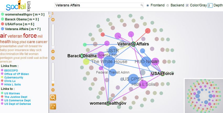
sual analytic browsing interface in Figure 8, which consists
of three parts, i.e. search input area on the top, information
5.2.2 Implementations summarization in the left column, and subgraph visualiza-
To improve the visual effect, we need to overcome the vi- tion in the main frame. After users input keywords in search
sual complexity of orbital layout, because it is a challenge box and select a focused vertex matching the keywords, our
to clearly present the cohesive subgraph with a large num- system visualizes the local subgraph in the main frame, so
ber of vertices. First, we set different colors to distinguish that users can select vertices they are interested in with the
vertices in different orbits. Retrospect the motivating exam- summarization in the left column. Without loss of gener-
ple in Figure 1b, it consists of four orbits in different colors ality, this example shows the 3-mutual-friend graph for the
representing vertices with four M values from 3 inside to 0 keyword “white house”, in which vertices represent twit-
outside. In order to distinguish vertices within one orbit, the ter actors and edges represent the “following” relationships.
size of vertices is proportional to vertex degree to reflect the The depth, equivalent to the distance threshold, is set to 2.
importance. For instance, vertex p has the largest degree so With the help of online algorithm and layout generation,
that it has the biggest size. we dramatically reduce the visual complexity in the main
Next, we consider how to visualize edges to further re- frame. The visible subgraph only contains 89 vertices and
duce the visual complexity. Since vertices within one orbit 527 edges, which is much smaller the initial local subgraph
may form several connected k-mutual-friend subgraphs, so with 2006 vertices and 2838 edges. As a result, we could
we carefully order vertices such that vertices belongs to one quickly perceive that the networking of “The White House”
subgraph are located successively on the orbit. As such, we is dominated by various US departments and government
can hide edges within one orbit without losing much con- officials, which is unlikely to obtain from thousands of ver-
nection information. As the Figure 1b shows, vertices g and tices with messy information. Furthermore, users can high-
h are near in the orbit and vertices j, k and l are near in light several vertices and their neighbors while other vertices
the orbit. Furthermore, inspired by the radial layout, we and edges become transparent. Considering in some cases
put a vertex close to connected vertices in the inner orbit subgraphs are quite large, users can use frontend search to
to minimize crossing edges. For example, vertices g and h locate preferred vertices within the current subgraph, or ad-
93Figure 8: Visual Analysis Interface
just the M value lower bound to filter out unsatisfied graph website7 . The datasets are sorted in increasing order of
elements using the slide bar at the top left corner. More- edge number. We utilize moderate size datasets (the first
over, we support zoom in/out function to focus on part of three) to compare in memory algorithms, while use large
the graph and users can view the sketch of the whole sub- size datasets (the last three) to compare algorithms in graph
graph with a thumbnail at the bottom right corner. database. Moreover, Twitter and DBLP datasets are se-
The left column displays the M values of the highlighted lected for online visual analysis since they contain rich tex-
vertices, the corresponding tag cloud as well as the link in- tual information.
formation for the vertex representing officials of “Veterans
Affairs”. The tag cloud is a helpful tool that summarizes Table 2: Dataset Statistics
the most significant and diverse topics in their tweets. In Dataset Vertex Edges Description
this example, we select 30 representative tags out of 100 Epinions 75k 405k Who-trusts-whom graph
candidates, where “Veterans Affairs” may show great con- Twitter 452k 813k Who-follows-whom graph
cern about the PTSD (Post Traumatic Stress Disorder) and DBLP 916k 3, 063k Who-cites-whom graph
discrimination problems while “womenshealthgov” mainly Flickr 1, 715k 22, 613k Flickr contact graph
focuses on topics like health, breast cancer and baby. In or- FriendFeed 653k 27, 811k Friendship graph
der to know the source of these tags, hovering over specific Facebook 72, 661k 160, 975k Friendship graph
tag in the tag cloud will trigger the source vertices being
highlighted. If we point to the “insurance” tag, the Twitter 6.1 Offline Computations Evaluation
actor “Barack Obama” will be highlighted indicating that
he pays close attention to the insurance issue. 6.1.1 Memory based Algorithms
We compare mNaive and mImproved algorithms on three
datasets and results are summarized in Figure 9. This fig-
ure depicts the effect of k on the response time of three
6. EXPERIMENTS datasets. For Epinions and DBLP datasets, mImproved
We present experimental studies to evaluate our social outperforms mNaive evidently, while their performances on
network visual analysis system in this section. For simpli- Twitter dataset are in the same level. This is because Twit-
fication, we refer to the intuitive algorithm in Section 4.1 ter dataset having average degree less than 2 is much more
as mNaive, Algorithm 1 as mImproved, while refer to Algo- sparse than the other two datasets. Therefore, even the
rithm 2 as dStream, Algorithm 4 as dPartition. The mOn- naive algorithm can reach the stable state very fast without
line is short for the online algorithm. We implement these incurring a great deal of unnecessary triangle computations.
algorithm in Java language and evaluate on the Windows For other two datasets, mImproved is about one order faster
operating system with Quad-Core AMD Opteron(tm) pro- than mNaive averagely.
cessor 8356 and 128GB RAM. One interesting observation is that the response time is
We compare our solutions on a great deal of real so- not quite related to k, but mainly determined by the triangle
cial network datasets described in Table 2, most of which
7
are collected from the Stanford Network Analysis Project’s http://snap.stanford.edu/
94350 mNaive 80 mNaive streaming based algorithm, and the response times for both
mImproved mImproved
300 70
of them are increasing with respect to the increase of graph
Response Time(s)
Response Time(s)
250 60
200
50 size. In particular, dStream algorithm is dominated by the
40
150
30
I/O time, while dPartition is dominated by the CPU time,
100 20 in accord with our analysis in Section 4.
50 10
0 0
In essence, the major difference between dStream and
1 2 3 4 5 1 2 3 4 5
k k dPartition is the cost for triangle computations. As shown in
(a) Epinions (b) Twitter Table 5, the average cost for triangle computations in dPar-
800 mNaive
tition is only one tenth of that in dStream, because most
mImproved
700 of the triangle computations in the former approach are in
Response Time(s)
600
500 memory while all the triangle computations in the later one
400 are in graph database. Comparing three datasets, the aver-
300
200 age triangle computing time for Facebook is the fastest for
100
0
both algorithms due to the smallest average degree of Face-
1 2 3 4 5
k book. As a result, although the number of edges in Facebook
(c) DBLP is much larger than that in FriendFeed, the response time of
Facebook is slightly larger than that of FriendFeed. More-
Figure 9: Comparison of Memory Algorithms
over, Table 6 summarizes the percentages of the partitioning
part and the computing part for dPartition algorithm. Be-
computing times in each algorithm, i.e. how many times the
cause the partitioning algorithm reads the input graph only
algorithm calls the triangle counting operator. As in the first
once and writes the partitions back to graph database, the
two rows in Table 3, the triangle computing times for Epin-
partitioning part costs small amount of time comparing to
ions dataset in mNaive is about ten times of that in mIm-
the computing part.
proved, which is close to the ratio of response time. Thus,
the result again justifies our conclusion in Section 4.1 that
Table 4: Number of Partitions in Algorithm 4
mImproved outperforms mNaive mainly because it largely
Flickr FriendFeed Facebook
reduces the amount of triangle computations. More specifi-
cally, when k = 1, because we only remove edges not in any Size(GB) 1.57 1.92 11.6
triangles without affecting other edges, mNaive can finish p 2 2 12
in two iterations (make sure that the graph is unchanged 90
in the second iteration), and mImproved only needs one it- 80
I/O Time
CPU Time
eration. The response time for mNaive decreases when k 70
Responce Time(h)
equals to 5 since the number of triangle computations drops 60
50
to 2, 439k, smaller than the number when k equals to 3 and 40
4. The triangle computing times for DBLP dataset in the 30
last two rows in Table 3 have the similar pattern. For Twit- 20
ter dataset, both algorithms need the number of triangle 10
computations in the same level, which determines that their 0
dS dP
trea artit
dS dP
trea artit
dS dP
trea artit
m ion m ion m ion
response time also close to each other. To sum up, mIm- Flickr FriendFeed Facebook
proved is much faster than mNaive mainly because it re-
duces the number of triangle computations, especially when Figure 10: Comparison of Disk Algorithms
the graph is dense. In conclusion, dPartition trades off a lightweight graph
partitioning for fast triangle computing in memory. The
Table 3: Triangle Computing Times result verifies our claim in Section 4 that the partition based
1 2 3 4 5 algorithm is I/O-efficient in practice.
mNaive 717k 2,219k 2,840k 3,088k 2,439k
mImproved 130k 202k 249k 284k 311k Table 5: 10k Times Triangle Computing Cost
mNaive 1,097k 1,261k 1,324k 1,364k 1,391k Dataset dStream dPartition
mImproved 873k 867k 836k 819k 817k Flickr 122.1s 11.3s
mNaive 5,950k 24,767k 22,950k 25,166k 21,085k FriendFeed 349.6s 33.5s
mImproved 288k 1,028k 1,921k 2,671k 3,240k
Facebook 12.9s 1.3s
6.1.2 Disk based Algorithms
Table 6: Percentages of Response Time
Next we evaluate the disk based algorithms with three
large scale datasets. For partition based algorithm, we con- Flickr FriendFeed Facebook
trol the usage of memory by only allowing to store a sub- Partitioning part 9.1% 10.5% 13.2%
graph with at most 1GB size. As such, we can estimate Computing part 90.9% 89.5% 86.8%
the number of partitions p for each dataset according to
the graph size in graph database as in Table 4. Since the re- 6.2 Online Analysis Evaluation
sponse time is not determined by k, we set k as 3 to compare By randomly selecting 10 focused vertices on Twitter and
the performance of two disk based algorithms. The results DBLP datasets respectively, we obtain the average perfor-
in Figure 10 depicts the response time for the three datasets mance of online analysis with three components: mOnline
with two parts: I/O time and CPU time. All in all, the algorithm, orbital layout generation and tag cloud selection.
partition based algorithm is about five times faster than the All the experiments are based on the 3-mutual-friend graph
95You can also read