Dynamics, behaviours, and anomaly persistence in cryptocurrencies and equities surrounding COVID-19 - arXiv
←
→
Page content transcription
If your browser does not render page correctly, please read the page content below
Dynamics, behaviours, and anomaly persistence in
                                               cryptocurrencies and equities surrounding COVID-19

                                                                                 Nick James
                                                   School of Mathematics and Statistics, University of Sydney, NSW, Australia
arXiv:2101.00576v2 [q-fin.ST] 10 Jan 2021

                                            Abstract
                                            This paper uses new and recently introduced methodologies to study the similarity
                                            in the dynamics and behaviours of cryptocurrencies and equities surrounding
                                            the COVID-19 pandemic. We study two collections; 45 cryptocurrencies and
                                            72 equities, both independently and in conjunction. First, we examine the
                                            evolution of cryptocurrency and equity market dynamics, with a particular focus
                                            on their change during the COVID-19 pandemic. We demonstrate markedly
                                            more similar dynamics during times of crisis. Next, we apply recently introduced
                                            methods to contrast trajectories, erratic behaviours, and extreme values among
                                            the two multivariate time series. Finally, we introduce a new framework for
                                            determining the persistence of market anomalies over time. Surprisingly, we
                                            find that although cryptocurrencies exhibit stronger collective dynamics and
                                            correlation in all market conditions, equities behave more similarly in their
                                            trajectories and extremes, and show greater persistence in anomalies over time.
                                            Keywords: Market dynamics, Cryptocurrency, Time series analysis, Nonlinear
                                            dynamics, COVID-19

                                            1. Introduction
                                                Over the last several years there has been growing interest in the cryptocur-
                                            rency market. The sector has experienced impressive growth in asset inflows and
                                            its level of sophistication. More recently, the COVID-19 pandemic has caused
                                            immense social and economic impacts, including changes in the behaviour of
                                            financial markets. The goal of this paper is to analyze the evolution of cryptocur-
                                            rencies and equities over time, and in particular, assess whether the increase in
                                            interest from sophisticated investors has led to more uniformity in the dynamics
                                            and behaviours of the two asset classes. We use the COVID-19 pandemic as a
                                            motivating example to ascertain whether this similarity changes during market
                                            crises.
                                                The study of financial market correlation structure has been a topic of great
                                            interest to the nonlinear dynamics community over the past several decades

                                                Email address: nicholas.james@sydney.edu.au (Nick James)

                                            Preprint submitted to Elsevier                                         January 12, 2021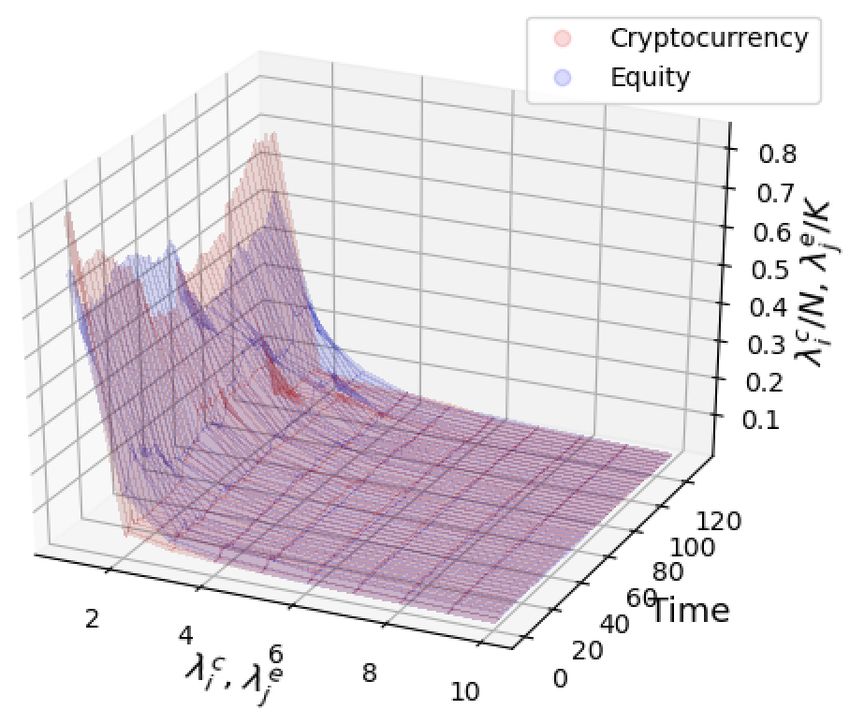
[1, 2, 3]. Evolutionary market dynamics have been studied through a wide variety
of techniques such as clustering [4] and principal components analysis (PCA)
[2, 5, 6, 7]. Until the past decade, the primary asset classes of interest to the
research community were equities [7], fixed income [8], and foreign exchange [9].
More recently, select research has focused on the study of trajectory modelling
[10], extreme behaviours and structural breaks [11, 12] and these methods have
been applied to a variety of asset classes.
    There is a current wave of interest from econophysics researchers in the
development and application of methods for understanding cryptocurrency
dynamics. Areas attracting interest from researchers include studies of Bitcoin’s
behaviour [13, 14, 15, 16, 17], fractal patterns, [18, 19, 20, 21], cross-correlation
and scaling effects [22, 23, 24, 25, 26]. Many of these studies are concerned with
the time-varying nature of such dynamics, or the behaviour of cryptocurrencies
during various market regimes. Quite naturally, the impact of COVID-19 on
cryptocurrency behaviours has been widely studied [27, 28, 29, 30]
    The evolution of COVID-19 and its impact on financial markets has attracted
broad interest from various research communities. COVID-19’s spread and
containment measures have been studied by the epidemiology community [31,
32, 33, 34, 35, 36, 37, 38, 39], while clinically-inclined research has detailed
new treatments for various COVID-19 strains [40, 41, 42, 43, 44, 45, 46]. The
pandemic’s varied impact on financial markets has also been studied [47, 48, 49],
with many papers exploring financial contagion and market stability [50, 51, 52].
In the nonlinear dynamics community, COVID-19 research has used new and
existing techniques to study the temporal evolution of cases and deaths [53, 54, 55,
56], with a substantial emphasis on SIR models [57, 58, 59, 60, 61, 62, 63], power
law models [64, 65, 66, 67] and the use of networks [68]. More recently there has
been work that explores the impact of COVID-19 cases on the performance of
country financial markets [10].
    The goal of this paper is to explore the similarity in the dynamics and
behaviours of cryptocurrencies and equities over the past two years. In doing so,
we make several contributions. First, we complement current methods with the
introduction of a new measure between eigenspectra to study the similarity in two
time series’ evolutionary dynamics. Next, we apply recently developed techniques
to study the trajectories, extremes and erratic behaviour of cryptocurrencies
and equities, and analyze their similarity. Finally, we introduce a pithy method
to study the persistence of financial anomalies over time.
    This paper is structured as follows. Section 2 describes the data used in
this paper. Section 3 studies the time-varying dynamics of cryptocurrencies and
equities, and contrasts their behaviour during different market states. Sections
4, 5 and 6 study trajectories, erratic behaviour and extremes respectively. In
Section 7 we contrast the consistency in anomalies among our two collections.
In Section 8, we conclude.

                                         2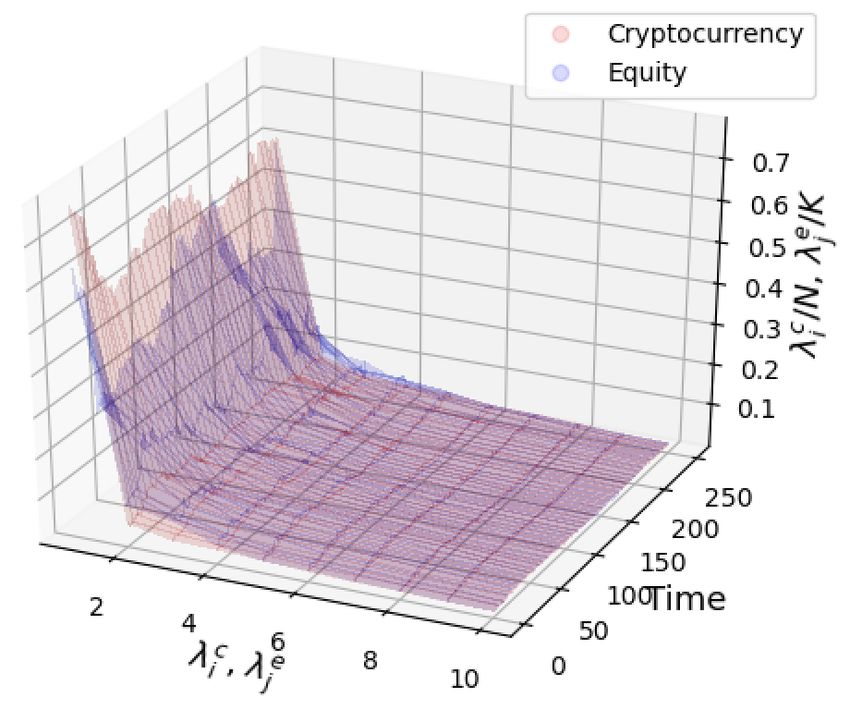
2. Data

   In the proceeding analysis, the two primary objects of study are cryptocur-
rency and equity multivariate time series between 03-12-2018 to 08-12-2020. We
analyze the 45 largest cryptocurrencies by market capitalisation (excluding those
previously identified as anomalous) [11] and 72 global equities whose market
capitalisation is greater than US$100 billion. We report and contrast on the
dynamics, behaviours, and anomaly persistence between cryptocurrencies and
equities. In select sub-sections, we refer to the period 03-12-2018 to 28-02-2020
as Pre-COVID, 02-03-2020 to 29-05-2020 as Peak COVID, and 01-06-2020 to
08-12-2020 as Post-COVID. Cryptocurrency and equity data are sourced from
https://coinmarketcap.com/ and Bloomberg respectively.

3. Market dynamics

3.1. Evolutionary dynamics
     In this section we follow the framework introduced in [1] to study the temporal
evolution of correlation structure in cryptocurrencies and equities, and contrast
these collections’ evolutionary dynamics. Our analysis in this section differs from
[1] in several ways, however. First, rather than applying this framework to a single
collection of securities from different asset classes, we apply the time-evolving
model to two separate asset classes (cryptocurrencies and equities) and compare
the respective time-varying dynamics. Second, we use a shorter time window
to study correlation structures, allowing correlations to change more quickly to
varying market conditions. This allows us to study the impact of COVID-19
on both collections. Third, we introduce a new dynamics deviation measure
between surfaces to determine the similarity in two time-varying eigenspectra
across different time periods. Finally, we use daily data rather than weekly data.
     Let ci (t) and ej (t) be the multivariate time series of cryptocurrency and
equity daily closing prices, for t = 1, ..., T , i = 1, ..., N , and j = 1, ..., K. We
generate two multivariate time series of log returns, Ric (t) and Rje (t), where
cryptocurrency and equity log returns are computed as follows

                                                  ci (t)
                               Ric (t) = log                ,                       (1)
                                               ci (t − 1)

                                                  ej (t)
                               Rje (t) = log                .                       (2)
                                               ej (t − 1)

   We define standardized  cryptocurrency returns as R̂ic (t) = [Ric (t)−hRic i]/σ(Ric ),
where σ(Ri ) = h(Ri ) i − hRic i2 represents the standard deviation of cryptocur-
          c
               p      c 2

rency time series Ric and h.i denotes an average over time. Standardized equity
returns are computed similarly and we denote this time series R̂je (t). Having
normalized the returns, we may construct empirical correlation matrices

                                           3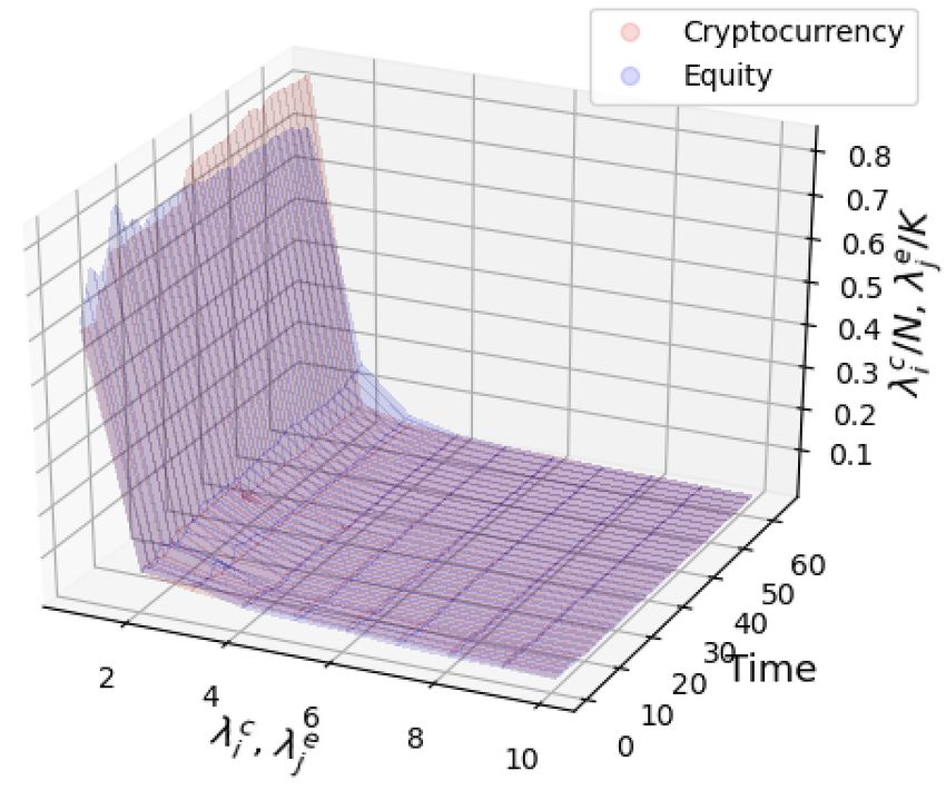
1 c cT
                                    Ωc =    R̂ R̂ ,                                    (3)
                                         T1
                                         1 e eT
                                    Ωe =    R̂ R̂ ,                                    (4)
                                         T1
    for cryptocurrency and equity time series. Elements of both correlation
matrices ω c (i, j) and ω e (i, j) lie ∈ [−1, 1]. We study the evolution of these
correlation matrices, using a rolling window of T1 = 60 days. One must be
judicious in the choice of the smoothing parameter T1 , as correlation coefficients
can be excessively smooth or noisy if T1 is too large or too small respectively.
Our choice of 60 days corresponds approximately to the length of the COVID-19
market crash. This allows us to capture the entirety of the COVID-19 market
shock, without including unrelated data outside the COVID-related crash in
our calculation. Next, we study the dynamics of the cryptocurrency and equity
market security collections by applying principal components analysis (PCA)
to the two time-varying correlation matrices. For each correlation matrix, we
wish to estimate the linear maps Φc and Φe that transform our standardized
cryptocurrency returns R̂c and equity returns R̂e into uncorrelated variables Z c
and Z e respectively. That is,

                                      Z c = Φc R̂c ,                                   (5)
                                        e
                                      Z = Φ R̂ .e   e
                                                                                       (6)

where the rows of Z c and Z e represent PCs of the matrices Rc and Re . The
rows of Φc and Φe , which contain PC coefficients, are ordered such that the
first rows are along the axes of most variation in the data, with subsequent PCs,
subject to the optimization constraint that they are all mutually orthogonal, each
accounting for maximal variance along their respective axes. The correlation
matrices, which are symmetric and diagonalizable matrices can be written in
the form
                                         1
                                   Ωc =    Λc Dc ΛTc ,                                 (7)
                                        T1
                                        1
                                   Ωe =    Λe De ΛTe ,                                 (8)
                                        T1
where Dc , De are diagonal matrices with eigenvalues λci , λej , and Λc , Λe are
orthogonal matrices with the associated eigenvectors from the cryptocurrency
and equity correlation matrices respectively. The PCs are estimated using the
diagonalizations above.
    Finally, we contrast the proportion of variance produced by a sub-collection
of eigenvalues within each of the two collections. The total variance of the
cryptocurrency returns R̂c and equity returns R̂e for the N and K assets
respectively, is equal to the sum of all eigenvalues λc1 + ... + λcN and λe1 + .... + λeK .
This is equivalently the trace of the two diagonal matrices of eigenvalues tr(Dc ) =
N and tr(De ) = K. To compute the proportion of total variance explained by

                                            4
(a) Cryptocurrency (b) Equity
Figure 1: Time-varying eigenspectrum for cryptocurrencies and equities.
the mth PC in R̂c and R̂e is therefore λ̃cm = λcm /N and λ̃em = λem /K. For more
details on this construction readers should visit [1, 69, 70].
Prior work has demonstrated that the eigenvector corresponding to the
largest eigenvalue represents the significance of ‘the market’ within the collection
[1]. Bearing this in mind, there are several noteworthy insights revealed in
Figure 1 regarding the similarity in cryptocurrency and equity dynamics. First,
both Figure 1a and Figure 1b exhibit a broadly similar shape; the majority
of explanatory variance is provided by the first several eigenvectors, with the
remaining proportion of total variance falling away quickly over the entire time
period. Next, the explanatory variance provided by the first cryptocurrency
eigenvalue λ̃c1 seen in figure 1a is consistently higher than the corresponding
equity market eigenvalue λ̃e1 in figure 1b. This demonstrates that the collective
force of the market is more pronounced in cryptocurrencies than equities during
our window of analysis. The second observation one may make from Figure 1
is the significant variability in λ̃e1 when compared with λ̃c1 . This may highlight
that within equity markets, there is more variability related to the market’s
impact on collective behaviour than that of cryptocurrencies. The time-varying
explanatory variance of the first PC is displayed in Figure 2, where λ̃c1 > λ̃e1 for
almost the entire window of analysis. Figure 2 indicates that the difference in
the first eigenvalue, |λ̃c1 − λ̃e1 |, is smallest during the Peak COVID period.
3.2. Dynamics surrounding COVID-19
In this section we study the similarity in the dynamics of cryptocurrencies
and equities during three discrete time periods which are characterized by
different systematic (market) risk profiles. Our goal is to determine whether
the similarity in cryptocurrency and equity market dynamics changes in varying
market conditions. The three periods are defined
• Pre-COVID: 03-01-2018 to 28-02-2020,
• Peak COVID: 02-03-2020 to 29-05-2020,
5Figure 2: Rolling explained variance ratio for cryptocurrencies λc1 /N and equities λe1 /K.
• Post-COVID: 01-06-2020 to 08-12-2020,
with corresponding lengths |TPRE |, |TPEAK | and |TPOST |. For the two sequences
of time-varying correlation matrices Ωct and Ωet , we study the similarity in the
explanatory variance of the first 10 eigenvalues. λ̃c1,t , ..., λ̃c10,t and λ̃e1,t , ..., λ̃e10,t .
We define the difference in these spectral surfaces dynamics deviation and
compute as follows
10
311 X
1 X
DDPRE = |λ̃ci,t − λ̃ei,t | (9)
|TPRE | t=60 i=1
375 X
10
1 X
DDPEAK = |λ̃ci,t − λ̃ei,t | (10)
|TPEAK | t=312 i=1
508 X
10
1 X
DDPOST = |λ̃ci,t − λ̃ei,t |. (11)
|TPOST | t=376 i=1
The measure is normalized by the length of each time period, allowing us to com-
pare dynamics during periods of varying lengths. As the majority of explanatory
variance is provided by the first 10 eigenvalues in both the cryptocurrency and
equity collections, we ignore the negligible difference in total variance explained
by the remaining elements of the eigenspectrum.
Figure 3 shows the cryptocurrency and equity eigenspectra during the three
windows of analysis. Of the three analysis windows, the two eigenspectra appear
to be most similar during the Peak COVID period, which is displayed in Figure
6(a) Pre Covid (b) Peak Covid
(c) Post Covid
Figure 3: Time-varying eigenspectrum Pre Covid, Peak Covid, and Post Covid.
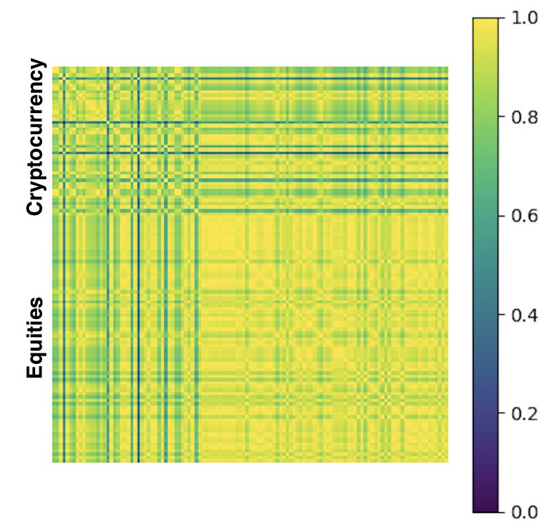
(a) Cryptocurrency (b) Equity
Figure 4: Kernel density estimates of wc (i, j) and we (i, j) from Pre Covid, Peak Covid and
Post Covid periods.
7Dynamics deviation scores
Period Score
DDPRE 0.369
DDPEAK 0.160
DDPOST 0.298
Table 1: Dynamics deviation from 3 periods of analysis
3b. This is confirmed in Table 1, which shows dynamics deviation scores for
the three windows of analysis. The results highlight a significant increase in the
similarity of the two collections’ collective behaviour during the Peak COVID
period, with a score of 0.160. The Pre-COVID and Post-COVID scores are 0.369
and 0.298 respectively, highlighting less similarity in the dynamics of equities
and cryptocurrencies outside periods of market crisis. This is primarily due to
the equity eigenspectrum’s first eigenvalue exhibiting lower explanatory variance
in the Pre-COVID and Post-COVID periods. This is shown in Figure 3a and
Figure 3c respectively.
Next, we contrast the cryptocurrency and equity correlation coefficients
during the same three windows of analysis seen in Figure 4. Figures 4a and
4b display kernel density estimates of cryptocurrency and equity correlation
matrix elements during the Pre-COVID, Peak COVID and Post-COVID periods.
There are two important insights. First, both cryptocurrency and equity markets
highlight a sharp increase in collective correlations during the Peak COVID
period. Both cryptocurrencies and equities displayed markedly lower correlation
coefficients in the Pre-COVID and Post-COVID periods. In all three periods,
cryptocurrency correlation coefficients were more strongly positive than that
of equities. These findings are consistent with the results in the Section 3.1,
where dynamics deviations were lowest during the Peak COVID market period;
suggesting that during market crises cryptocurrency and equity behaviours are
most similar.
4. Trajectory modelling
In this section, we study the trajectory dynamics [71] of equity and cryp-
tocurrency closing prices for the entirety of our time period, a single period of
T = 508 days. To compare trajectories of securities with markedly different
prices, we normalize the cryptocurrency time series ci (t) and equity time series
ej (t). Analyzing a candidate individual cryptocurrency provides a function
PT
ci ∈ RT . We let kci k1 = t=1 |ci (t)| be the L1 norm of the function, and define
a normalized cryptocurrency price trajectory by Tci = kcciik1 . Similarly, we define
PT
kej k1 = t=1 |ej (t)|, and the corresponding normalized equity trajectory as
ej
Tj = kej k1 . Distances between such vectors highlight the relative change in cryp-
e
tocurrency and equity securities during the time period. To study such changes,
we define two trajectory matrices, DijTC
= kTci − Tcj k1 and DijTE
= kTei − Tej k1 ,
and perform hierarchical clustering.
8First, we compare norms of the two trajectory matrices to better understand
similarity within each collection. Both of these matrices are symmetric, real
and have trace 0. As the two collections are of different sizes, we normalize the
norm computations by the number of elements in each trajectory matrix.qP The
normalized cryptocurrency trajectory matrix norm kD k2 = N
TC ∗ −1 tc 2
i,j |dij |
qP
and the normalized equity trajectory matrix norm kDT E k2∗ = K −1 i,j |dij | .
te 2
The normalized cryptocurrency trajectory matrix norm kDT C k2∗ = 0.4804 and
the normalized equity trajectory matrix norm kDT E k2∗ = 0.1849, demonstrating
more similarity in normalized trajectories among equities than cryptocurrencies.
There are several possible explanations for this finding. First, there could be
some bias in our sample of equities, having chosen the 72 largest equities in
the world by market capitalization. It is likely that the volatility in their price
behaviour will be less than that of smaller equities. On the other hand, this
finding may quite reasonably reflect the volatile nature of cryptocurrency market
sentiment. Although correlations among the cryptocurrency constituents are
higher than that of equity constituents, the consistently strong influence of ‘the
market’ may make trajectories highly responsive to sharp changes in sentiment.
Figures 5 and 6 display the cryptocurrency and equity trajectory dendrograms
respectively. Each dendrogram highlights several noteable insights regarding
trajectory clusters. Figure 5 shows two major clusters, a predominant cluster
with high self-similarity, a smaller more amorphous cluster and a single outlier in
Revain. The predominant cluster contains most cryptocurrencies analyzed with
less volatile price trajectories. The smaller cluster is composed of cryptocurren-
cies having exhibited major volatility in their price trajectory, such as Chainlink,
which experienced a price increase of almost 42 times during our window of anal-
ysis. This dendrogram has markedly different structure to the equity trajectory
dendrogram, shown in Figure 6. The equity trajectory dendrogram exhibits
more substantial self-similarity, with three clearly defined clusters; one predomi-
nant cluster and two smaller, well-defined clusters exhibiting high self-similarity.
The first minority cluster contains stocks such as; Microsoft, Amazon, Alibaba,
Tencent, Facebook, Apple and TSMC - all of which are technology companies.
The second small cluster contains stocks such as: Chevron, Exxon, BP, Shell,
Wells Fargo and HSBC - primarily financial services and energy companies. Both
of these sectors tend to perform well in buoyant equity markets, and badly in
declining markets. The largest, most predominant third cluster contains the
remaining equities. The growth in passive and factor based investing may have
increased the similarity in these equities’ behaviours, as investors increasingly
seek to buy stocks within a sector or ‘theme’ of the market.
5. Erratic behaviour modelling
In this section we study the similarity of structural breaks in our two mul-
tivariate time series of log returns, Ric (t) and Rje (t) defined earlier. For each
security in the respective time series, we apply the two-phase change point detec-
tion algorithm described by [72] to generate a set of structural breaks for each
9Figure 5: Hierarchical clustering on DT C .
Figure 6: Hierarchical clustering on DT E .
10log return time series. Each change point represents a point in time where the
algorithm determines the statistical properties of the time series to have changed.
We apply the Kolmogorov-Smirnov test, detecting general distributional changes
in the underlying time series. The change point detection method could instead
focus on changes in specific distributional moments such as mean or variance,
however. We obtain two collections of finite sets ξ1c , ..., ξN c
, and ξ1e , ..., ξK
e
for
cryptocurrency and equity time series respectively, where all sets are a subset of
{1, ..., T }.
Next, we compute distances between the cryptocurrency structural break sets
ξic and equity structural break sets ξje . There is significant literature highlighting
issues in using metrics such as the Hausdorff distance, due to its sensitivity to
outliers, [73, 74] and so we use a recently introduced semi-metric modification
[74] between candidate sets within our two collections of structural breaks ξic
and ξje . Normalized distances between sets of cryptocurrencies are computed:
c
P c
!
b∈ξjc d(b, ξi )
P
1 a∈ξic d(a, ξj )
c c
D(ξi , ξj ) = + , (12)
2 |ξjc | |ξic |
where d(b, ξic ) is the minimal distance from b ∈ ξjc to the set ξic . Distances
between sets of equities are computed similarly:
e
P e
!
b∈ξje d(b, ξi )
P
1 a∈ξie d(a, ξj )
e e
D(ξi , ξj ) = + , (13)
2 |ξje | |ξie |
where d(b, ξie ) is the minimal distance from b ∈ ξje to the set ξie . This semi-
metric is the L1 norm average of all minimal distances between any two sets.
As all time series are of equal length, it is not necessary to normalize by the
length of the time series. Finally, we form two breaks matrices between sets of
cryptocurrency structural breaks, Dij BC
= D(ξic , ξjc ) and equity structural breaks,
Dij = D(ξi , ξj ). To better understand collective similarity in structural breaks,
BE e e
we perform hierarchical clustering on our two breaks matrices.
Like Section 4, we compare norms of the two distance matrices to better
understand breaks similarity within each collection. As the two collections
are of different sizes, again, we normalize the two norm computations by the
size of the distance matrix.
qP The normalized cryptocurrency breaks matrix
norm kDBC k2∗ = N −1 i,j |dij | and the normalized equity breaks matrix
bc 2
qP
norm kDBE k2∗ = K −1 i,j |dij | . The normalized cryptocurrency breaks
be 2
matrix norm kDBC k2∗ = 23.42 and the normalized equity breaks matrix norm
kDBE k2∗ = 23.88, highlighting approximately equivalent similarity in structural
breaks among equities and cryptocurrencies. This result is consistent with earlier
findings [11], which suggest that although one collection of time series may exhibit
more volatility and possibly warrant a higher number of structural breaks, the
univariate nature of the change point detection algorithm [72] detects structural
breaks relative to the properties of the particular time series. Therefore, although
11Figure 7: Hierarchical clustering on DBC .
Figure 8: Hierarchical clustering on DBE .
12cryptocurrency time series may exhibit more volatility, the behaviour in their
collective structural breaks is not necessarily more or less similar than that of
the equity collection.
Next, we compare the cluster structures of the two collections. The cryptocur-
rency breaks dendrogram, seen in Figure 7 consists of one primary cluster with
three, diffuse sub-clusters. The primary cluster has one predominant sub-cluster
of concentrated similarity, with the three remaining, smaller clusters having a
more indeterminate form. By contrast, the equity breaks dendrogram in Figure
8 has a more easily interpreted cluster structure. There are four small clusters,
each of which contains two or three equities, and a predominant cluster which is
comprised of the remaining equities. The four small clusters appear to cluster
based on sector, where cluster one consists of Facebook and Comcast (technol-
ogy), cluster two consists of BP and Shell (energy), cluster three consists of
Merck and Amgen (biotechnology/pharmaceuticals), and cluster four consists of
Tencent, Apple and Microsoft (technology). These results suggest that, with the
exception of select equities within specific sectors that exhibit similar structural
break patterns, most equities have similar structural breaks behaviour.
6. Extreme behaviour modelling
In this section, we study anomalies with respect to total returns and extreme
behaviors within our collections of cryptocurrencies and equities. First, we
outline the procedure to measure distance between extreme values of candidate
time series. We let µ be a probability distribution that stores the extreme values
of a cryptocurrency time series ci (t) or equity time series ej (t). We assume
that µ is a continuous probability measure of the form µ = f (x)dx, where dx is
Lebesgue measure, and f (x) is a probability density function that is non-negative
everywhere and integrates to 1. We study the 10% and 90% points of density,
respectively, by the equations
Z l
f (x)dx = 0.1 (14)
−∞
Z ∞
f (x)dx = 0.1 (15)
u
The range x ≤ l gives the most extreme 10% of the distribution on the left side
of the distribution, while the range x ≥ u gives the 10% right most extreme
values. The restricted function is defined
f (x), x ≤ l
g(x) = f (x)1{x≤l}∪{x≥u} = 0, l < x < u (16)
f (x), x ≥ u.
Next, we construct an associated measure ν = g(x)dx, with dx as Lebesgue
measure. We generate N associated probability measures µc1 , ..., µcN , and returns
measures ν1c , ..., νN
c
for our cryptocurrency time series. Similarly we generate
13(a) AR (b) AE
Figure 9: Affinity matrices returns and extremes.
K probability measures µe1 , ..., µeK , and return measure ν1e , ..., νK e
for our equity
time series. As all restricted measures are of total size 0.2, we use the Wasserstein
metric to compute distances between these truncated distributions. Finally, we
form a matrix between the distributional extremities of all time series. Let
DijEC
= dw (νic , νjc ) be the matrix between the cryptocurrency extreme return
distributions, and Dij EE
= dw (νie , νje ) be the matrix between equity extreme
return distributions. PT
We define total returns for cryptocurrencies zic = t=1 Ric (t) and equities
T
zje = t=1 Rje (t). We now compute returns matrices for cryptocurrency returns,
P
Dij = |zic − zjc | and equity returns Dij
RC RE
= |zie − zje |. To identify anomalies with
respect to returns and extreme values, we transform the four distance matrices
into affinity matrices. That is, a candidate affinity matrix A, is defined as
Dij
Aij = 1 − , (17)
max {D}
where A is symmetric, Aii = 1, 0 ≤ Aij ≤ 1, ∀i, j. We now define an affinity
returns matrix AR and an affinity extremes matrix AE both of which are of
dimension 117 x 117, which include all 45 cryptocurrencies and 72 equities
analyzed in this paper.
We study Figure 9 and compare collective similarities in returns and extremes
among our two collections. Figure 9a shows the affinity returns matrix AR . It
is clear that both equities and cryptocurrencies exhibit strong self-similarity,
with the equity collection exhibiting slightly more similar returns than the
cryptocurrency collection. Although not as strong as the intra-asset similarity,
there is still reasonable similarity in the returns profile between that of equities
and cryptocurrencies. Figure 9b displays a clear difference in the collective
behaviours. Similarly to returns, equities exhibit more self-similarity than that of
14Figure 10: Elements κc (s, t) and κe (s, t).
cryptocurrencies. However unlike returns, there is markedly less similarity when
comparing the extremes of cryptocurrencies and equities. These findings are
consistent with the results presented in Sections 4 and 5, where cryptocurrencies
were shown to be more varied in their trajectories and less consistent in their
structural breaks. This finding supports the high degree of dependence identified
between extreme and erratic behaviour in the cryptocurrency market.
7. Anomaly persistence
In this section, we study the evolution of ranks among cryptocurrencies and
equities with respect to risk-adjusted returns. Rather than using correlation, we
apply the concept of ranks, as financial analysts often apply ‘ranking’ systems
when identifying anomalous securities (equities, bonds, currencies, Petc.). We
P t c t e
t−60 Ri (t) t−60 Rj (t)
define rolling risk-adjusted returns κci (t) = σic (t) and κej (t) = σje (t)
where σic (t) and σje (t) are the standard deviations of rolling cryptocurrency and
equity log returns for t ∈ {61, ..., T }. Like Section 3, we use a rolling window of
60 days and record two time-evolving sequences of risk adjusted return ranks.
Given rank vectors s, t ∈ {61, ..., T }, we define K c (s, t) and K e (s, t) as matrices
measuring the Kendall rank correlation coefficient between any two risk-adjusted
return rank vectors s and t for all possible points in time. A higher score indicates
more similarity in the securities exhibiting high and low risk-adjusted returns
at any two points in time. Elements of both matrices k c (s, t) and k e (s, t) lie
∈ [−1, 1].
First, we study the norms of the two anomaly persistence matrices kK c k2 =
15(a) K c (s, t) (b) K e (s, t)
Figure 11: Anomaly persistence matrices K c (s, t) and K e (s, t).
qP qP
s,t |kst | and kK k2 =
c 2 e e |2 . The cryptocurrency anomaly persis-
|kst
s,t
tence norm, kK c k2 = 109.69 and the equity anomaly persistence norm kK e k2
= 122.62. The higher score for the equity collection suggests that there is
more consistency in the stocks that are anomalous on a risk-adjusted return
basis over time. Figure 10 which plots two distributions of the elements k c (s, t)
and k e (s, t), demonstrates a higher average correlation for equities than that of
cryptocurrencies. Further interesting structure over time is revealed in Figure
11.
Both Figures 11a and 11b have high correlation scores around the diagonal,
which is indicative of short-term dependence in anomalous behaviours within
both collections. However, Figure 11b clearly displays a higher level of similarity
over time - indicating more persistence in anomalous behaviours. This is further
supported in our hierarchical clustering analysis, where the dendrograms for
K c (s, t) and K e (s, t) are displayed in Figure 12. There are two primary takeaways
from this analysis. First, K e (s, t) is demonstrably more positive than K c (s, t)
for the vast majority of the dendrogram. This indicates that there is greater
similarity in risk-adjusted return ranks, over all comparative measurements in
time, for our collection of equities. Second, the K e (s, t) dendrogram determines a
total of 9 clusters, while K c (s, t) has a total of 11 clusters. This finding indicates
more stability in equity rank correlation scores over the entirety of our analysis
window.
16(a) K c (s, t)
(b) K e (s, t)
Figure 12: Hierarchical clustering on anomaly persistence matrices K c (s, t) and K e (s, t).
178. Conclusion
Our work in Section 3 demonstrates that collective dynamics in the cryp-
tocurrency market are significantly stronger than that of the equity market. The
explanatory variance provided by the largest eigenvector is consistently larger,
and more stable among cryptocurrencies than equities. Partitioning our analysis
into three discrete windows highlights that collective dynamics are most similar
between our two collections during the Peak COVID period, demonstrating that
equities and cryptocurrencies behave most similarly during market crises. This is
further supported in our correlation matrix analysis, where both cryptocurrencies
and equities experience a sharp increase in their correlations during the peak of
COVID-19. In periods surrounding the crisis (Pre-COVID and Post-COVID),
cryptocurrency correlation coefficients are more strongly positive than that of
equities.
Section 4 examines the similarity in normalized price trajectories among
both collections. Distance matrix norms indicate that equities exhibit more
similarity among their trajectories than cryptocurrencies. This may be due to
the significant price volatility exhibited by cryptocurrencies over the past two
years, making their trajectories (generally, but not universally) more dissimilar.
Hierarchical clustering on both time series displays marked differences in cluster
structures. Equity trajectories display more self-similarity than cryptocurrencies.
We suspect that the latent phenomenon may be the growth of passive and
factor-based investing over the last several years.
Section 5 compares the similarity in erratic behaviour among equities and
cryptocurrencies. Distance matrix norms display comparable similarity in the
erratic behaviours of cryptocurrencies and equities. Although cryptocurrencies
may be more volatile, the univariate nature of our changepoint detection algo-
rithm is unable to determine structural breaks with respect to the rest of the
collection. Using other change point detection methodologies to detect structural
breaks [75] may result in different findings.
Our results in Section 6 are consistent with those in Section 4. Figure 9 shows
more homogeneity among equity extremes in comparison to cryptocurrencies.
Analyzing distance matrix norms and affinity matrices highlights a substantial
difference in self-similarity. When contrasting the similarity in all 117 time series
for total returns and extreme values, the distinction in extreme value similarity
is most evident.
Finally in Section 7, equities are shown to exhibit more persistent anomalies
than cryptocurrencies. We apply hierarchical clustering to our proposed anomaly
persistence matrix. Hierarchical clustering determines the existence of 9 and 11
clusters respectively in the K c (s, t) and K e (s, t). A lower number of clusters
signals greater consistency in anomaly ranks over time. This is further supported
analyzing the elements of our matrix, which indicate a higher correlation in
anomaly rankings over time in the equity time series.
This work bridges several disparate areas of research: nonlinear dynamics,
econophysics, COVID-19 and cryptocurrency market dynamics. There are several
interesting avenues for future research. First, our analysis could be applied to
18more asset classes beyond cryptocurrencies and equities. Second, other techniques
could be introduced to study phenomena such as: market dynamics, trajectories,
extreme and erratic behaviour, and anomaly persistence. Finally, this analysis
could be run on different time windows and on a more timely basis. The chaotic
and non-deterministic nature of financial markets necessitates timely research
on topics of interest.
Acknowledgements
I would like to thank Peter Radchenko and Max Menzies for helpful discus-
sions.
19Appendix A. Mathematical objects glossary
Mathematical objects table: Section 3
Object Description
N # cryptocurrency time series
K # equity time series
ci (t) Cryptocurrency price time series
ej (t) Equity price time series
Ric (t) Cryptocurrency returns time series
Rje (t) Equity returns time series
R̂ic (t) Standardized cryptocurrency returns time series
R̂je (t) Standardized equity returns time series
Ωc Cryptocurrency correlation matrix
Ωe Equity correlation matrix
ω c (i, j) Element (i, j) in cryptocurrency correlation matrix
ω e (i, j) Element (i, j) in equity correlation matrix
Φc Cryptocurrency PC coefficient matrix
Φe Equity PC coefficient matrix
Zc Cryptocurrency PC matrix
Ze Equity PC matrix
Dc Cryptocurrency diagonal matrix
De Equity diagonal matrix
λc Cryptocurrency eigenvalues
λe Equity eigenvalues
Λc Cryptocurrency orthogonal eigenvector matrix
Λe Equity orthogonal eigenvector matrix
λ̃c Cryptocurrency eigenvalue explanatory variance
λ̃e Equity eigenvalue explanatory variance
|TPRE | Length of Pre-COVID period
|TPEAK | Length of Peak COVID period
|TPOST | Length of Post-COVID period
DDPRE Pre-COVID dynamics deviation
DDPEAK Peak COVID dynamics deviation
DDPOST Post-COVID dynamics deviation
Table A.2: Mathematical objects and definitions
20Mathematical objects table: Sections 4, 5, 6, 7
Object Description
Tci Cryptocurrency normalized price trajectory
Tej Equity normalized price trajectory
DT C Cryptocurrency trajectory matrix
DT E Equity trajectory matrix
kDT C k2∗ Normalized cryptocurrency trajectory matrix norm
kDT E k2∗ Normalized equity trajectory matrix norm
ξ1c , ..., ξN
c
Cryptocurrency structural break sets
e
ξ1 , ..., ξKe
Equity structural break sets
D BC
Cryptocurrency breaks matrix
DBE Equity breaks matrix
kDBC k2∗ Normalized cryptocurrency breaks matrix norm
kDBE k2∗ Normalized equity breaks matrix norm
DEC Cryptocurrency extremes matrix
DEE Equity extremes matrix
zic (t) Cryptocurrency total returns time series
zje (t) Equity total returns time series
DRC Cryptocurrency returns matrix
DRE Equity returns matrix
AR Affinity returns matrix (Cryptocurrencies and equities)
AE Affinity extremes matrix (Cryptocurrencies and equities)
κc (t) Cryptocurrency risk-adjusted return vector at time t
κe (t) Equity risk-adjusted return vector at time t
σic (t) Cryptocurrency realized volatility at time t
σje (t) Equity realized volatility at time t
K c (s, t) Cryptocurrency anomaly persistence matrix
K e (s, t) Equity anomaly persistence matrix
k c (s, t) Element (s, t) in cryptocurrency anomaly persistence matrix
k e (s, t) Element (s, t) in equity anomaly persistence matrix
kK c k2 Cryptocurrency anomaly persistence matrix norm
kK e k2 Equity anomaly persistence matrix norm
Table A.3: Mathematical objects and definitions
21Appendix B. Securities analyzed
Cryptocurrency tickers and names
Ticker Coin Name Ticker Coin Name
BTC Bitcoin THETA THETA
ETH Ethereum MKR Maker
XRP XRP SNX Synthetix
LINK Chainlink OMG OMG Network
BCH Bitcoin Cash DOGE Dogecoin
ADA Cardano ONT Ontology
BNB Binance Coin DCR Decred
XLM Stellar BAT Basic Attention
BSV Bitcoin SV NEXO Nexo
EOS EOS ZRX 0x
XMR Monero REN Ren
TRX Tron QTUM Qtum
XEM NEM ICX ICON
XTZ Tezos LRC Loopring
NEO NEO Token KNC Kyber Network
VET VeChain REP Augur
REV Revain Classic LSK Lisk
DASH Dash BTG Bitcoin Gold
WAVES Waves SC Siacoin
HT Huobi Token QNT QUANT
MIOTA IOTA MAID MaidSafeCoin
ZEC ZCash NANO Nano
ETC Ethereum Classic
Table B.4: Cryptocurrency tickers and names
22Equity tickers and names
Ticker Equity Name Ticker Equity Name
NYSE: C Citigroup EPA: OR L’Oreal
NYSE: MRK Merck NYSE: UNH UnitedHealth Group
NYSE: KO Coca-Cola EPA: FP Total
NASDAQ: AMGN Amgen SHA: 601988 Bank of China
NYSE: T AT&T SHA: 601288 A.B. China
LON: BATS British American Tobacco LON: HSBA HSBC
NYSE: JPM JP Morgan Chase NYSE: VZ Verizon
TYO: 7203 JP Toyota Motor NYSEARCA: SPY SPDR S&P 500
ASX: CBA CBA NYSE: SLB Schlumberger
SHA: 601939 China Construction Bank EPA: SAN Sanofi
NASDAQ: CSCO Cisco NYSE: IBM IBM
NYSE: MDT Medtronic NYSE: PG Procter & Gamble
LON: BP BP NASDAQ: FB Facebook
NYSE: BRK Berkshire Hathaway SHA: 601398 ICBC
SWX: NOVN Novartis SHA: 600028 Sinopec
ETR: SIE Siemens NASDAQ: MSFT Microsoft
NYSE: WMT Walmart NYSE: WFC Wells Fargo
NYSE: DIS Walt Disney SWX: RO Roche Holdings
NYSE: JNJ Johnson and Johnson NASDAQ: PEP PepsiCo
NASDAQ: INTC Intel NYSE: PFE Pfizer
NYSE: GE General Electric NYSE: XOM Exxon Mobil
NASDAQ: AAPL Apple NYSE: BMY Bristol-Myers Squibb
NYSE: GS Goldman Sachs NASDAQ: CMCSA Comcast
KRX: 005930 Samsung Electronics NYSE: HD Home Depot
HKG: 0941 China Mobile NYSE: MA Mastercard
NASDAQ: AMZN Amazon LON: ULVR Unilver
NYSE: ORCL Oracle SWX: NESN Nestle
NYSE: MMM 3M NYSE: V Visa
AMS: RDSA Royal Dutch Shell NYSE: PM Philip Morris
BME: ITX INDITEX NYSE: ABBV AbbVie Inc
NYSE: MO Altria Group HKG: 9988 Alibaba
NYSE: CVX Chevron NASDAQ: KHC Kraft Heinz
TSE: RY Royal Bank of Canada NASDAQ: GOOGL Alphabet
HKG: 0700 Tencent EBR: ABI Anheuser Busch Inbev NV
TPE: 2330 TSMC NYSE: BAC Bank of America
ETR: SAP SAP SHA: 601857 PetroChina
Table B.5: Equity tickers and names
Appendix C. Change point detection algorithm
In this section, we provide an outline of change point detection algorithms, and
describe the specific algorithm that we implement. Many statistical modelling
problems require the identification of change points in sequential data. By
23definition, these are points in time at which the statistical properties of a time
series change. The general setup for this problem is the following: a sequence
of observations x1 , x2 , ..., xn are drawn from random variables X1 , X2 , ..., Xn
and undergo an unknown number of changes in distribution at points τ1 , ..., τm .
One assumes observations are independent and identically distributed between
change points, that is, between each change points a random sampling of the
distribution is occurring. Following Ross [72], we notate this as follows:
F0 if i ≤ τ1
F if τ < i ≤ τ
1 1 2
Xi ∼
F 2 if τ2 < i ≤ τ3,
...
While this requirement of independence may appear restrictive, dependence can
generally be accounted for by modelling the underlying dynamics or drift process,
then applying a change point algorithm to the model residuals or one-step-ahead
prediction errors, as described by Gustafsson [76]. The change point models
applied in this paper follow Ross [72].
Appendix C.1. Batch change detection (Phase I)
This phase of change point detection is retrospective. We are given a fixed
length sequence of observations x1 , . . . , xn from random variables X1 , . . . , Xn .
For simplicity, assume at most one change point exists. If a change point exists
at time k, observations have a distribution of F0 prior to the change point, and
a distribution of F1 proceeding the change point, where F0 6= F1 . That is, one
must test between the following two hypotheses for each k:
H0 : Xi ∼ F0 , i = 1, ..., n
(
F0 i = 1, 2, ..., k
H1 : Xi ∼
F1 , i = k + 1, k + 2, ..., n
and end with the choice of the most suitable k.
One proceeds with a two-sample hypothesis test, where the choice of test
is dependent on the assumptions about the underlying distributions. To avoid
distributional assumptions, non-parametric tests can be used. Then one ap-
propriately chooses a two-sample test statistic Dk,n and a threshold hk,n . If
Dk,n > hk,n then the null hypothesis is rejected and we provisionally assume that
a change point has occurred after xk . These test statistics Dk,n are normalised
to have mean 0 and variance 1 and evaluated at all values 1 < k < n, and the
largest value is assumed to be coincident with the existence of our sole change
point. That is, the test statistic is then
D̃k,n − µD̃k,n
Dn = max Dk,n = max
k=2,...,n−1 k=2,...,n−1 σD̃k,n
24where D̃k,n were our unnormalised statistics.
The null hypothesis of no change is then rejected if Dn > hn for some
appropriately chosen threshold hn . In this circumstance, we conclude that a
(unique) change point has occurred and its location is the value of k which
maximises Dk,n . That is,
τ̂ = argmax Dk,n .
k
This threshold hn is chosen to bound the Type 1 error rate as is standard in
statistical hypothesis testing. First, one specifies an acceptable level α for the
proportion of false positives, that is, the probability of falsely declaring that a
change has occurred if in fact no change has occurred. Then, hn should be chosen
as the upper α quantile of the distribution of Dn under the null hypothesis. For
the details of computation of this distribution, see [72]. Computation can often
be made easier by taking appropriate choice and storage of the Dk,n .
Appendix C.2. Sequential change detection (Phase II)
In this case, the sequence (xt )t≥1 does not have a fixed length. New ob-
servations are received over time, and multiple change points may be present.
Assuming no change point exists so far, this approach treats x1 , ..., xt as a fixed
length sequence and computes Dt as in phase I. A change is then flagged if
Dt > ht for some appropriately chosen threshold. If no change is detected, the
next observation xt+1 is brought into the sequence. If a change is detected, the
process restarts from the following observation in the sequence. The procedure
therefore consists of a repeated sequence of hypothesis tests.
In this sequential setting, ht is chosen so that the probability of incurring
a Type 1 error is constant over time, so that under the null hypothesis of no
change, the following holds:
P (D1 > h1 ) = α,
P (Dt > ht |Dt−1 ≤ ht−1 , ..., D1 ≤ h1 ) = α, t > 1.
In this case, assuming that no change occurs, the average number of observations
received before a false positive detection occurs is equal to α1 . This quantity
is referred to as the average run length, or ARL0. Once again, there are
computational difficulties with this conditional distribution and the appropriate
values of ht , as detailed in Ross [72].
25References
[1] D. J. Fenn, M. A. Porter, S. Williams, M. McDonald, N. F. Johnson, N. S.
Jones, Temporal evolution of financial-market correlations, Physical Review
E 84 (2011). doi:10.1103/physreve.84.026109.
[2] L. Laloux, P. Cizeau, J.-P. Bouchaud, M. Potters, Noise dressing of financial
correlation matrices, Physical Review Letters 83 (1999) 1467–1470. doi:10.
1103/physrevlett.83.1467.
[3] M. C. Münnix, T. Shimada, R. Schäfer, F. Leyvraz, T. H. Seligman, T. Guhr,
H. E. Stanley, Identifying states of a financial market, Scientific Reports 2
(2012). doi:10.1038/srep00644.
[4] A. J. Heckens, S. M. Krause, T. Guhr, Uncovering the dynamics of
correlation structures relative to the collective market motion, Journal
of Statistical Mechanics: Theory and Experiment 2020 (2020) 103402.
doi:10.1088/1742-5468/abb6e2.
[5] D.-H. Kim, H. Jeong, Systematic analysis of group identification in stock
markets, Physical Review E 72 (2005). doi:10.1103/physreve.72.046133.
[6] R. K. Pan, S. Sinha, Collective behavior of stock price movements in an
emerging market, Physical Review E 76 (2007). doi:10.1103/physreve.76.
046116.
[7] D. Wilcox, T. Gebbie, An analysis of cross-correlations in an emerging
market, Physica A: Statistical Mechanics and its Applications 375 (2007)
584–598. doi:10.1016/j.physa.2006.10.030.
[8] J. Driessen, B. Melenberg, T. Nijman, Common factors in international bond
returns, Journal of International Money and Finance 22 (2003) 629–656.
doi:10.1016/s0261-5606(03)00046-9.
[9] M. Ausloos, Statistical physics in foreign exchange currency and stock
markets, Physica A: Statistical Mechanics and its Applications 285 (2000)
48–65. doi:10.1016/s0378-4371(00)00271-5.
[10] N. James, M. Menzies, Association between COVID-19 cases and interna-
tional equity indices, Physica D: Nonlinear Phenomena 417 (2021) 132809.
doi:10.1016/j.physd.2020.132809.
[11] N. James, M. Menzies, J. Chan, Changes to the extreme and erratic
behaviour of cryptocurrencies during COVID-19, Physica A: Statistical
Mechanics and its Applications 565 (2021) 125581. doi:10.1016/j.physa.
2020.125581.
[12] Ş. Telli, H. Chen, Structural breaks and trend awareness-based interaction
in crypto markets, Physica A: Statistical Mechanics and its Applications
558 (2020) 124913. doi:10.1016/j.physa.2020.124913.
26[13] J. Chu, S. Nadarajah, S. Chan, Statistical analysis of the exchange rate
of Bitcoin, PLOS ONE 10 (2015) e0133678. doi:10.1371/journal.pone.
0133678.
[14] S. Lahmiri, S. Bekiros, A. Salvi, Long-range memory, distributional variation
and randomness of bitcoin volatility, Chaos, Solitons & Fractals 107 (2018)
43–48. doi:10.1016/j.chaos.2017.12.018.
[15] D. Kondor, M. Pósfai, I. Csabai, G. Vattay, Do the rich get richer? an
empirical analysis of the Bitcoin transaction network, PLoS ONE 9 (2014)
e86197. doi:10.1371/journal.pone.0086197.
[16] A. F. Bariviera, M. J. Basgall, W. Hasperué, M. Naiouf, Some stylized facts
of the Bitcoin market, Physica A: Statistical Mechanics and its Applications
484 (2017) 82–90. doi:10.1016/j.physa.2017.04.159.
[17] J. Alvarez-Ramirez, E. Rodriguez, C. Ibarra-Valdez, Long-range correlations
and asymmetry in the Bitcoin market, Physica A: Statistical Mechanics and
its Applications 492 (2018) 948–955. doi:10.1016/j.physa.2017.11.025.
[18] D. Stosic, D. Stosic, T. B. Ludermir, T. Stosic, Multifractal behavior of price
and volume changes in the cryptocurrency market, Physica A: Statistical
Mechanics and its Applications 520 (2019) 54–61. doi:10.1016/j.physa.
2018.12.038.
[19] D. Stosic, D. Stosic, T. B. Ludermir, T. Stosic, Exploring disorder and
complexity in the cryptocurrency space, Physica A: Statistical Mechanics
and its Applications 525 (2019) 548–556. doi:10.1016/j.physa.2019.03.
091.
[20] S. A. Manavi, G. Jafari, S. Rouhani, M. Ausloos, Demythifying the be-
lief in cryptocurrencies decentralized aspects. A study of cryptocurrencies
time cross-correlations with common currencies, commodities and financial
indices, Physica A: Statistical Mechanics and its Applications 556 (2020)
124759. doi:10.1016/j.physa.2020.124759.
[21] P. Ferreira, L. Kristoufek, E. J. de Area Leão Pereira, DCCA and DMCA
correlations of cryptocurrency markets, Physica A: Statistical Mechanics and
its Applications 545 (2020) 123803. doi:10.1016/j.physa.2019.123803.
[22] S. Drozdz, R. Gebarowski, L. Minati, P. Oswiecimka, M. Wactorek, Bitcoin
market route to maturity? Evidence from return fluctuations, temporal
correlations and multiscaling effects, Chaos: An Interdisciplinary Journal
of Nonlinear Science 28 (2018) 071101. doi:10.1063/1.5036517.
[23] S. Drozdz, L. Minati, P. Oswiecimka, M. Stanuszek, M. Watorek, Signatures
of the crypto-currency market decoupling from the forex, Future Internet
11 (2019) 154. doi:10.3390/fi11070154.
27[24] S. Drozdz, L. Minati, P. Oswiecimka, M. Stanuszek, M. Wactorek, Compe-
tition of noise and collectivity in global cryptocurrency trading: Route to
a self-contained market, Chaos: An Interdisciplinary Journal of Nonlinear
Science 30 (2020) 023122. doi:10.1063/1.5139634.
[25] R. Gębarowski, P. Oświęcimka, M. Wątorek, S. Drożdż, Detecting cor-
relations and triangular arbitrage opportunities in the forex by means of
multifractal detrended cross-correlations analysis, Nonlinear Dynamics 98
(2019) 2349–2364. doi:10.1007/s11071-019-05335-5.
[26] M. Wątorek, S. Drożdż, J. Kwapień, L. Minati, P. Oświęcimka, M. Stanuszek,
Multiscale characteristics of the emerging global cryptocurrency market,
Physics Reports (2020). doi:10.1016/j.physrep.2020.10.005.
[27] S. Corbet, C. Larkin, B. Lucey, The contagion effects of the COVID-19
pandemic: Evidence from gold and cryptocurrencies, Finance Research
Letters 35 (2020) 101554. doi:10.1016/j.frl.2020.101554.
[28] T. Conlon, R. McGee, Safe haven or risky hazard? bitcoin during the
covid-19 bear market, Finance Research Letters 35 (2020) 101607. doi:10.
1016/j.frl.2020.101607.
[29] T. Conlon, S. Corbet, R. J. McGee, Are cryptocurrencies a safe haven for
equity markets? an international perspective from the COVID-19 pandemic,
Research in International Business and Finance 54 (2020) 101248. doi:10.
1016/j.ribaf.2020.101248.
[30] Q. Ji, D. Zhang, Y. Zhao, Searching for safe-haven assets during the COVID-
19 pandemic, International Review of Financial Analysis 71 (2020) 101526.
doi:10.1016/j.irfa.2020.101526.
[31] G. Wang, Y. Zhang, J. Zhao, J. Zhang, F. Jiang, Mitigate the effects of
home confinement on children during the COVID-19 outbreak, The Lancet
395 (2020) 945–947. doi:10.1016/s0140-6736(20)30547-x.
[32] M. Chinazzi, et al., The effect of travel restrictions on the spread of the
2019 novel coronavirus (COVID-19) outbreak, Science 368 (2020) 395–400.
doi:10.1126/science.aba9757.
[33] Y. Liu, A. A. Gayle, A. Wilder-Smith, J. Rocklöv, The reproductive number
of COVID-19 is higher compared to SARS coronavirus, Journal of Travel
Medicine 27 (2020). doi:10.1093/jtm/taaa021.
[34] Y. Fang, Y. Nie, M. Penny, Transmission dynamics of the COVID-19
outbreak and effectiveness of government interventions: A data-driven
analysis, Journal of Medical Virology 92 (2020) 645–659. doi:10.1002/jmv.
25750.
28[35] P. Zhou, et al., A pneumonia outbreak associated with a new coron-
avirus of probable bat origin, Nature 579 (2020) 270–273. doi:10.1038/
s41586-020-2012-7.
[36] J. Dehning, J. Zierenberg, F. P. Spitzner, M. Wibral, J. P. Neto, M. Wilczek,
V. Priesemann, Inferring change points in the spread of COVID-19 reveals
the effectiveness of interventions, Science 369 (2020) eabb9789. doi:10.
1126/science.abb9789.
[37] N. Ferguson, D. Laydon, G. Nedjati Gilani, N. Imai, K. Ainslie, M. Baguelin,
S. Bhatia, A. Boonyasiri, Z. Cucunuba Perez, G. Cuomo-Dannenburg,
A. Dighe, I. Dorigatti, H. Fu, K. Gaythorpe, W. Green, A. Hamlet, W. Hins-
ley, L. Okell, S. Van Elsland, H. Thompson, R. Verity, E. Volz, H. Wang,
Y. Wang, P. Walker, P. Winskill, C. Whittaker, C. Donnelly, S. Riley,
A. Ghani, Report 9: Impact of non-pharmaceutical interventions (npis) to re-
duce covid19 mortality and healthcare demand (2020). doi:10.25561/77482.
[38] C. Wang, L. Liu, X. Hao, H. Guo, Q. Wang, J. Huang, N. He, H. Yu,
X. Lin, A. Pan, S. Wei, T. Wu, Evolving epidemiology and impact of
non-pharmaceutical interventions on the outbreak of coronavirus disease
2019 in Wuhan, China (2020). doi:10.1101/2020.03.03.20030593.
[39] B. F. Maier, D. Brockmann, Effective containment explains subexponential
growth in recent confirmed COVID-19 cases in china, Science 368 (2020)
742–746. doi:10.1126/science.abb4557.
[40] F. Jiang, L. Deng, L. Zhang, Y. Cai, C. W. Cheung, Z. Xia, Review
of the clinical characteristics of Coronavirus Disease 2019 (COVID-19),
Journal of General Internal Medicine 35 (2020) 1545–1549. doi:10.1007/
s11606-020-05762-w.
[41] Z. Y. Zu, M. D. Jiang, P. P. Xu, W. Chen, Q. Q. Ni, G. M. Lu, L. J.
Zhang, Coronavirus disease 2019 (COVID-19): A perspective from China,
Radiology (2020) 200490. doi:10.1148/radiol.2020200490.
[42] G. Li, E. D. Clercq, Therapeutic options for the 2019 novel coronavirus
(2019-nCoV), Nature Reviews Drug Discovery 19 (2020) 149–150. doi:10.
1038/d41573-020-00016-0.
[43] L. Zhang, Y. Liu, Potential interventions for novel coronavirus in China:
A systematic review, Journal of Medical Virology 92 (2020) 479–490.
doi:10.1002/jmv.25707.
[44] M. Wang, R. Cao, L. Zhang, X. Yang, J. Liu, M. Xu, Z. Shi, Z. Hu,
W. Zhong, G. Xiao, Remdesivir and chloroquine effectively inhibit the
recently emerged novel coronavirus (2019-nCoV) in vitro, Cell Research 30
(2020) 269–271. doi:10.1038/s41422-020-0282-0.
[45] B. Cao, et al., A trial of Lopinavir-Ritonavir in Covid-19, New England
Journal of Medicine 382 (2020) e68. doi:10.1056/nejmc2008043.
29[46] L. Corey, J. R. Mascola, A. S. Fauci, F. S. Collins, A strategic approach
to COVID-19 vaccine R&D, Science 368 (2020) 948–950. doi:10.1126/
science.abc5312.
[47] D. Zhang, M. Hu, Q. Ji, Financial markets under the global pandemic of
COVID-19, Finance Research Letters (2020) 101528. doi:10.1016/j.frl.
2020.101528.
[48] Q. He, J. Liu, S. Wang, J. Yu, The impact of COVID-19 on stock markets,
Economic and Political Studies (2020) 1–14. doi:10.1080/20954816.2020.
1757570.
[49] A. Zaremba, R. Kizys, D. Y. Aharon, E. Demir, Infected markets: Novel
coronavirus, government interventions, and stock return volatility around
the globe, Finance Research Letters 35 (2020) 101597. doi:10.1016/j.frl.
2020.101597.
[50] M. Akhtaruzzaman, S. Boubaker, A. Sensoy, Financial contagion during
COVID–19 crisis, Finance Research Letters (2020) 101604. doi:10.1016/j.
frl.2020.101604.
[51] D. I. Okorie, B. Lin, Stock markets and the COVID-19 fractal contagion
effects, Finance Research Letters (2020) 101640. doi:10.1016/j.frl.2020.
101640.
[52] S. Lahmiri, S. Bekiros, The impact of COVID-19 pandemic upon stability
and sequential irregularity of equity and cryptocurrency markets, Chaos,
Solitons & Fractals 138 (2020) 109936. doi:10.1016/j.chaos.2020.109936.
[53] S. Khajanchi, K. Sarkar, Forecasting the daily and cumulative number of
cases for the COVID-19 pandemic in India, Chaos: An Interdisciplinary
Journal of Nonlinear Science 30 (2020) 071101. doi:10.1063/5.0016240.
[54] M. H. D. M. Ribeiro, R. G. da Silva, V. C. Mariani, L. dos Santos Coelho,
Short-term forecasting COVID-19 cumulative confirmed cases: Perspectives
for Brazil, Chaos, Solitons & Fractals 135 (2020) 109853. doi:10.1016/j.
chaos.2020.109853.
[55] T. Chakraborty, I. Ghosh, Real-time forecasts and risk assessment of novel
coronavirus (COVID-19) cases: A data-driven analysis, Chaos, Solitons &
Fractals 135 (2020) 109850. doi:10.1016/j.chaos.2020.109850.
[56] N. James, M. Menzies, Cluster-based dual evolution for multivariate time
series: Analyzing COVID-19, Chaos: An Interdisciplinary Journal of
Nonlinear Science 30 (2020) 061108. doi:10.1063/5.0013156.
[57] A. Ballesteros, A. Blasco, I. Gutierrez-Sagredo, Hamiltonian structure of
compartmental epidemiological models, Physica D: Nonlinear Phenomena
413 (2020) 132656. doi:10.1016/j.physd.2020.132656.
30You can also read