Summertime and the drivin' is easy? Daylight Saving Time and vehicle accidents - Ioannis Laliotis, Guiseppe Moscelli & Vassilis Monastiriotis ...

LSE ‘Europe in Question’ Discussion Paper Series

Summertime and the drivin’ is easy?
Daylight Saving Time and vehicle
accidents

Ioannis Laliotis, Guiseppe Moscelli & Vassilis
Monastiriotis

LEQS Paper No. 150/2019

December 2019

Ioannis Laliotis, Guiseppe Moscelli & Vassilis Monastiriotis

 Editorial Board
 Dr Bob Hancké
 Dr Vassilis Monastiriotis
 Dr Sonja Avlijas
 Dr Cristóbal Garibay-Petersen
 Dr Pieter Tuytens
 Mr Toon Van Overbeke

All views expressed in this paper are those of the author(s) and do not necessarily represent
the views of the editors or the LSE.

© Ioannis Laliotis, Guiseppe Moscelli, and Vassilis Monastiriotis

Daylight Savings Time and Car Accidents

Summertime and the drivin’ is easy?

Daylight Savings Time and vehicle accidents

Ioannis Laliotis *, Guiseppe Moscelli **,
and Vassilis Monastirioris ***

Abstract

Although it is commonly understood that light conditions affect driving behaviour, detailed
evidence is scarce especially for EU countries. In this paper we use the exogenous
variation in daylight caused by Daylight Saving Time (DST) shifts to examine the role of
light conditions on vehicle accidents. We use a rich dataset from Greek administrative data
covering the universe of all types of recorded vehicle accidents over the period between
01 January 2006 to 32 December 2016. Relying on a regression discontinuity design we
attempt to provide a casual evaluation regarding the impact of exogenous time shifts on
the number of vehicle crashes. Our results are supportive of an ambient light mechanism
that reduces the counts of serious vehicle accidents during the Spring transitions and
increases on the count of minor ones during the Fall transition, especially during the most
impacted hours within the day. We discuss the implications of our study both for the
importance of light ambience conditions for car accidents and for the particular case of
the adoption and preservation of DST policies.

Keywords: DST, Driving behaviour, vehicle accidents Greece

JEL Codes: I12; I18; R41

*** Department of Economics, City, University of London
 Email: Ioannis.Laliotis@city.ac.uk
*** School of Economics, University of Surrey
 Email: g.moscelli@surrey.ac.uk
*** European Institute, London School of Economics and Political Science
 Email: v.monastiriotis@lse.ac.uk

Ioannis Laliotis, Guiseppe Moscelli & Vassilis Monastiriotis

Table of Contents

1. Introduction........................................................................... 1

2. Data ...................................................................................... 4

3. Estimation Strategy ............................................................... 8

4. Results ................................................................................ 10
 4.1 Baseline estimates................................................................................................................ 10

 4.2 Ambient light mechanism ..................................................................................................... 15

 4.3 Sleep deprivation mechanism .............................................................................................. 17

 4.4 Crash factors ......................................................................................................................... 18

 4.5 Omitted variables .................................................................................................................. 20

 4.6 Implications ........................................................................................................................... 22

5. Conclusions ........................................................................ 26

References ............................................................................... 29

Appendix .................................................................................. 31

Ioannis Laliotis, Guiseppe Moscelli & Vassilis Monastiriotis

1. Introduction

It is rather unproblematic to imagine that differences in ambient light conditions affect

driving capacity and hence, the incidence of vehicle accidents. However, causal

evidence about this relationship is scarce, especially for EU countries. Indeed, on

March 2019 the European Parliament voted for the abolition of seasonal clock changes

by 2021, with member states keeping their right to decide on their time zone after that.

The European Parliament had previously requested an ex-post evaluation of Directive

2000/84/EC regulating transition into and out of Summer Time in the EU countries
(Anglmayer, 2017). Based on the findings of that study the European Parliament called

on the European Commission to consider abolishing Daylight Saving Time (DST) for

their member countries.

Among other potential implications, the report raised concerns about the impact of

DST on road safety, mainly due to sleep deprivation and ambient light conditions.1

Their recommendations relied on studies for the UK and the US which, however,

arrived at mixed conclusions. The UK literature review suggested that collision risk

reduces (increases) when entering (exiting) DST (Carey and Sarma, 2017). The US
study used a regression discontinuity design to show that fatalities increase when

entering DST through a lack of sleep mechanism that affects both drivers and

pedestrians (Smith, 2016). As the European Parliament report suggested, the existing

evidence on the issue is too thin – both regrading the transferability of the above
findings to mainland European countries, due to different climate and ambient light

conditions, and more generally. Our paper seeks to fill this gap, by providing detailed

1 The report mentioned a number of other effects – for example, that DST causes health
inconveniences through disruptions of the circadian rhythm of individuals (Kantermann et al.,
2007) – but concluded that Summer Time is overall beneficial, as it benefits the transport sector
and outdoor leisure activities and marginally reduces energy consumption. In the empirical
economics literature, transition into DST has also been shown to increase heart attack
incidences (Janszky and Ljung, 2008; Toro et al., 2015) and to exert a negative influence on life
satisfaction and mood (Kountouris and Remoundou, 2014; Sexton and Beatty, 2014).

1

Daylight Savings Time and Car Accidents

evidence on how exogenous variations in daylight ambience, due to DST shifts, affect

vehicle accidents.

Transitions into and out of DST may affect individual driving behaviour through two

major channels. The first one is by redistributing sunlight within the day. During the

Spring transition, one hour of sunlight is reallocated from the morning to the evening.

This creates a darker and riskier driving environment during the morning and one

with better light conditions during the evening, while all other working and
commuting schedules and patterns remain unchanged. During the Fall transition the

extra hour of evening sunlight is returned back to the morning, hence creating a darker

atmosphere in the evening. Light conditions have been shown to affect the circadian

rhythm and drowsiness of drivers (Chipman and Jin, 2009). A recent study by
Bünnings and Schiele (2018) for England, Scotland and Wales shows that darker

environments are associated with increased year-round road safety costs. Thus,

variation in ambient light conditions could be associated with the number of vehicle

crashes.

An alternative channel through which DST shifts affect driving behaviour is sleep

deprivation. Recent research has shown that DST causes significant behavioural

changes, especially during the Spring transition. Individuals sleep less, on average,

due to moving clocks on hour forward and they tend to spend more time at home in

the morning and less time at home during the evening (Sexton and Beatty, 2014).2

Sleep deprivation affects the level of alertness and there is experimental evidence

regarding a negative relationship with driving performance (Otmani et al., 2005; Philip

et al., 2005).Therefore, DST transitions could affect road safety via both channels. This
could have important implications because vehicle accidents are a significant source

of external mortality. According to data for the period 2000-2016 provided by the

2The amount of sleep loss is 15-20 minutes according to Sexton and Beatty (2014). In a previous
study, Barnes and Wagner (2009) used the same dataset (American Time Use Survey) and
found that individuals sleep 40 minutes less, on average, on the night of Spring transition. Both
studies showed that sleep gains during the Fall transition are not statistically significant.

 2

Ioannis Laliotis, Guiseppe Moscelli & Vassilis Monastiriotis

Hellenic Statistical Authority, more than 1,500 people die every year from vehicle

accidents although this figure follows a declining trend since 2006. On average, this

represents nearly 1.5% of the overall annual mortality in the country. However, apart

from the extreme case of a fatal crash, there are lots of other implications associated

with vehicle accidents. These include deterioration in general health status, greater use

of healthcare and other public services, increased insurance premia, absence from

work, foregone earnings, post-traumatic stress etc.

In this study we provide three main contributions to the literature. First and foremost,

we attempt a causal evaluation of DST shifts on road accidents focusing on Greece, in

order to provide further and updated empirical evidence for an EU member state. To

this end, we use a very rich administrative dataset that has not been used for this
purpose before, at least to our knowledge. Under a special licence agreement with the

Hellenic Statistical Authority, we obtained detailed data on all reported vehicle

accidents in Greece during the period between 01 January 2006 and 31 December 2016.

Second, but quite importantly, unlike previous studies we consider the whole
distribution of vehicle accidents (i.e. minor, non-fatal/serious and fatal ones) and not

only a small portion of accidents causing fatalities Smith (2016). Third, our rich data

allow us to provide an original heterogeneity analysis of the DST effects on road

accidents depending on weather conditions, drinking behaviour, road type and

economic conditions, thus allowing for a clearer identification of the DST impact.

As a country state of the European Economic Community, Greece adopts Daylight

Saving Time since 1975. On the last Sunday of March each year, time in all member

countries is set forward by one hour at 01:00 Greenwich Mean Time (GMT) until the
last Sunday of October when it is set backwards by one hour at 01:00 GMT. Therefore,

randomisation needed to identify the causal impact relies on the natural experiment

generated by entering and leaving DST (Imbens and Lemieux, 2008). Using a sharp

regression discontinuity design, we examine whether entering into DST affects various
types of traffic accidents. The results indicate that entering into DST does not have any

significant implication on the daily counts of total and minor accidents. There is a

3

Daylight Savings Time and Car Accidents

significant reduction in the daily count of serious accidents and a weak and imprecise

increase for fatal accidents. Analysing the crash count by within-day hour intervals

reveals that the reduction in serious crashes occurs during hours that are affected the

most by the reallocation of sunlight into the evening. Regarding transitions back to the

Standard Time in the Fall, our results suggest an increased count for total crashes,

driven by a statistically significant increase in minor accidents. This result is stronger

for the evening hours, which in this case are the ones to be affected the most by
reallocating an hour of sunlight back in the morning. The ambient light mechanism is

also supported by examining separately night accidents taking place in adequately lit

locations versus locations with inadequate or no street lights. These results are backed

up by an extensive series of robustness checks and falsification tests that we exploit in
the paper.

The remainder of the paper is organised as follows: Section 2 outlines the data and

presents some descriptive evidence regarding patterns in the data. Section 3 describes

the empirical strategy and some basic assumptions. Section 3 discusses the results and
Section 5 concludes.

 2. Data

Under a signed agreement with the Hellenic Statistical Authority (EL.STAT hereafter),
we were granted access to information extracted from the universe of the Road

Accidents Reports for the period between 01 January 2006 and 31 December 2016 in

Greece. The inspecting road police officers fill in those reports after every vehicle

accident. During their inspection, all aspects regarding the crash are recorded. Those

refer to the type and severity of the accident and its precise date, time and location.

According to the severity variable, an accident is classified as either fatal, serious or

minor. A vehicle crash is defined as fatal if it resulted in the death of an involved

individual within 30 days from the crash. By reporting results for non-fatal accidents,

our study supplements the evidence provided by Smith (2016), who estimated the

impact of DST on fatal crashes only. Moreover, information about the driver such as

 4

Ioannis Laliotis, Guiseppe Moscelli & Vassilis Monastiriotis

gender, age, nationality, and the year they got their driving license is also collected.

They also report whether they conducted any alcohol tests and the corresponding

results. Details about the vehicles involved in the accident such as their type, safety

features (airbags, seatbelts etc.), and manufacture year is collected as well. Inspecting

officers also report information on weather conditions as well as the street light

conditions for accidents occurring during night hours. Finally, they report information

regarding the type of the road network an accident took place, e.g. whether it was
highway, within a residential area, its number of lanes etc.

To address any concern regarding the fact that the first Sunday under DST is one hour

shorter than the remaining days, we follow Smith (2016) and adjust the crash counts

by several alternative ways. First, we counted the 03:00-04:00 hour twice, using it as a
proxy for the missing 02:00-03:00 hour on the DST entering day. At the same time, we

divided the crashes occurred from 01:00 to 02:00 by two on the DST exit day as this

hour occurs twice on every Fall transition. Second, we multiplied Spring transition

date crashes by 24/23. Because that specific date has only 23 hours, crash counts were
inflated under the assumption that they evolve smoothly over the day. Fall transition

date crashes were multiplied by 24/25. Third, we dropped the transition dates from

the estimation sample. Regardless of the adjustment type chosen, our results remained

identical to those obtained when using the officially recorded count of vehicle crashes.

In our estimations we use crash counts aggregated by day or hour interval. The main

reason behind this aggregation is the scarcity of vehicle crashes, especially for fatal

and serious ones. Regarding the total period, minor accidents represent 87.7% of the

total, while serious and fatal accidents stand for 7.1% and 5.2% of the total count,
respectively. Table 1 presents descriptive statistics by crash type. During the total

period, the average daily count of total vehicle accidents in the country is 37, with a

minimum of 8 and a maximum of 73 crashes. The total crashes distribution is mainly

shaped by the minor accidents one. Fatal and serious accidents are rarer. Their daily
averages are 1.9 and 2.6, respectively. Figure A1, in the appendix, displays the

distribution and the daily profile for each type of accident. Distributions provide

5

Daylight Savings Time and Car Accidents

evidence regarding the rarity of fatal and serious crashes.3 Aggregation to national-

level time series also smooths out any confounders specific to weather conditions and

other characteristics that could affect the daily crash count for a specific location but

for not the total country.

 Table 1. Descriptive statistics for accident variables.

 Mean Std. Dev. Min. Max. Observations

 (1) (2) (3) (4) (5)

 Total accidents 37.14 9.59 8 73 4,018

 Fatal accidents 1.93 1.52 0 10 4,018
 Serious accidents 2.65 1.87 0 14 4,018

 Minor accidents 32.56 8.45 7 66 4,018
 Source: Hellenic Statistical Authority (EL.STAT). Notes: Daily averages for the period between 01 Jan
 2006 and 31 Dec 2016.

Hourly profiles suggest that vehicle accidents are more frequent during the evening

and night hours as compared to morning ones, although fatal and serious counts are

more uniformly distributed throughout the day. As previous studies have suggested,

substituting ambient light from low traffic frequency hours, i.e. during the early

morning hours, to high frequency ones, i.e. during the early evening, could indeed be

a cost-effective policy in terms of road casualties (Broughton et al., 1999). Further

descriptive evidence regarding the raw accidents data is provided in Table 2. Mean

daily counts from the first week of both transitions are compared to mean counts from

one week before and one week after. Moreover, in order to account for seasonal trends,

counts from the first week after each transition are benchmarked against averages

obtained using one and two weeks before and after. In general, it seems that there is a

small accidents reduction when adopting DST in the Spring. Differences are less

pronounced when returning back to Standard Time in the fall.

3Originally, there were 74 administrative regions in our data. However, all vehicle crash types
had a region-specific mode equal to zero.

 6

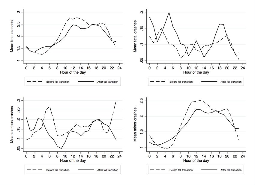
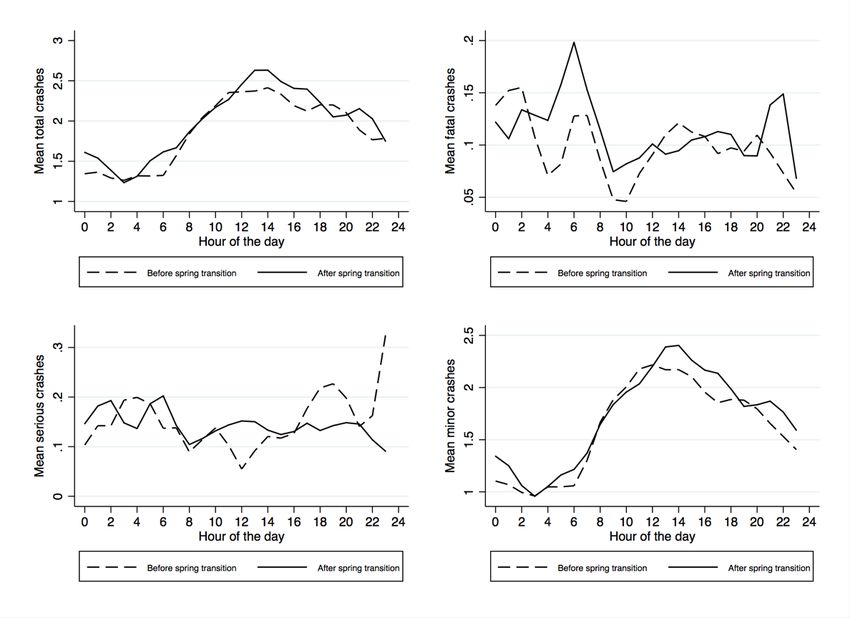
Ioannis Laliotis, Guiseppe Moscelli & Vassilis Monastiriotis

 Table 2. Mean accidents counts before and after transition.
 1 week 2 weeks
 (1) (2) (3) (4)
 before and (5)
 before and
 Panel A: Spring
 First week 1 transition
 week 1 week after after after
 Mean total crash count 33.74 34.77
 before 37.42 36.09 36.05
 t-test relative to 1st - .505 .009 .061 .044
 week
 Mean fatal crash count 1.68 1.87 2.12 1.99 1.91
 t-test relative to 1st - .399 .053 .114 .212
 week
 Mean serious crash 2.34 2.49 2.49 2.49 2.46
 count
 t-test relative to 1st - .566 .520 .488 .565
 week

 Mean minor crash 29.73 30.40 32.81 31.60 31.68
 count

 t-test relative to 1st - .626 .017 .099 .056
 week
 Panel B: Fall transition
 Mean total crash count 37.25 38.08 35.00 36.54 37.31
 t-test relative to 1st - .573 .118 .578 .953
 week
 Mean fatal crash count 1.83 2.04 1.90 1.97 1.90

 t-test relative to 1st - .402 .782 .502 .708
 week
 Mean serious crash 2.71 2.44 2.40 2.42 2.45
 count
 t-test relative to 1st - .360 .320 .255 .255
 week
 Mean minor crash 32.70 33.60 30.70 32.15 32.97
 count

 t-test relative to 1st - .497 .123 .629 .796
 week
 Observations 77 77 77 154 308
 Source: Hellenic Statistical Authority (EL.STAT). Authors’ calculations.

In order to examine whether changes during transitions vary within the day, we

plotted the mean crash count by hour using a 5-day time window before and after each

transition. This will provide some indications on whether differences vary around the

clock, especially for hours that are more or less affected by moving clocks backwards

and forward. Figure A2 displays the results. Regarding Spring transition (panel A) it

7

Daylight Savings Time and Car Accidents

seems that for total accidents the effects are small. However, there is a decrease in

serious accidents in the evening, and an increase in fatal accidents in the morning

hours during the Spring transition. Panel B graphs the hour-specific means before and

after the Fall transition. Regarding fatal accidents, they seem increased during the

evening hours on the first days after falling back to Standard Time, while serious

crashes appear to decrease during the morning hours.

 3. Estimation Strategy

The causal effect of DST on counts of various vehicle accident types is evaluated via a

regression discontinuity (RD) design strategy. Our identification relies on a natural

experiment based on the standard practice of advancing clocks by one hour each

Spring and then moving them backwards by one hour in the Fall. This generates an

exogenous reallocation of sunlight from the morning to the evening and vice versa.

Figure A3 plots the sunrise and sunset times (solid lines) alongside with their

respective counterfactuals in the absence of the DST practice (dotted lines). Advancing
clocks forward when entering and adjusting them backwards when exiting DST

generates an exogenous variation in the supply of daylight, especially around sunrise

and sunset. Either through the sleep deprivation or the ambient light conditions

mechanism, this variation could have implications on driving behaviour and hence,
the number of vehicle accidents. Under this framework, we compare the count of car

crashes that occur before entering DST to the count of crashes that occur after. As

explained in the Data section, at first we collapse the dataset in order to construct daily

time series of accident counts covering the total period. Using those data series, we

estimate reduced-form models of the following form:

 ℎ '( = + + - '( + 2 '( 5 + 2 '( × '( 5 + '( (1)

 8

Ioannis Laliotis, Guiseppe Moscelli & Vassilis Monastiriotis

In this baseline model specification ℎ '( is the count of accidents (either total,

fatal, serious or minor ones) on day i, and year y. '( is a binary indicator switched

on conditional that the i-th day falls under the DST period in the y-th year.

 '( is the running variable measuring the number of days before and after

the DST transition, i.e. it is centered on the transition dates in each year. Finally, f is a

function of the running variable and u is the disturbance term. Our models control for

a series of variables in order to eliminate effects due to day-of-week, general time
trends and public holidays (Smith, 2016; Toro et al., 2015). In our preferred empirical

specification, we use local Poisson regressions at both sides of the transition date

cutoff, a uniform kernel and optimal data-driven bandwidths (Calonico et al., 2014).

Compared to high order polynomials of the running variable, local linear regressions
have been shown to perform better in RD settings (Gelman and Imbens, 2018; Smith,

2016). The robustness of the results is confirmed using also higher order polynomials

as well as alternative kernels and bandwidths. In this framework, the coefficient of

interest is - and it measures the overall DST effect on vehicle accidents right at the

transition date. By using Poisson regressions we avoid any kind of transformation of

the dependent variable. A log-transformation of the number of crashes would be

problematic with our data since the number of fatal and serious crashes is zero for

some days, but also because the conventional use of estimating log-linearised models

with transformed dependent variables via OLS has been shown to produce biased

estimates (Santos Silva and Tenreyro, 2006), especially under the presence of

heteroscedasticity. The effect of entering DST on vehicle accidents is identified under

the assumptions that factors influencing driving behaviour and vehicle accidents,

other than the DST, are continuous at the transition dates. To this end, we test for

discontinuities at the transition dates for fuel prices and vehicle miles travelled using

data obtained from various sources. We also report results from falsification tests

using placebo transition dates in order to provide support regarding the validity of the
estimates. Moreover, we make use of several accidents features contained in the Road

Accident Reports in order to explore possible mechanisms that drive the results,

through the heterogeneity of roads conditions or driver’s drinking behaviour.

9

Daylight Savings Time and Car Accidents

4. Results

4.1 Baseline estimates
We first present some graphical evidence regarding the impact of DST on vehicle

crashes. We regress each crash count on day-of-week, month, year and public holiday

fixed effects, using local Poisson regressions. 4 The obtained response residuals are
then averaged by day over the total period covered by the data. Figure A4 presents the

results. There is a clear drop in serious crashes and a weaker increase for fatal crashes

at the Spring transition date (panel A). Regarding the Fall transition, in panel B, there

is a visible increase for total accidents, driven by the jump in minor accidents, as well
as a drop for serious accidents.

Table 3 reports the estimated size of those breaks observed at the Spring transition for

each accident type. For robustness we report estimates using regressions with first and

second order polynomials of the running variable around the cutoff date, uniform and

triangular kernels and optimally data-driven bandwidths (Calonico et al., 2014). As

indicated in the graphical evidence, there is not a significant discontinuity for total and

minor accidents in panels A and D, respectively. The estimated baseline effect of DST

on fatal crashes (panel B) is positive, in line with the effect uncovered in the US study
(Smith, 2016). However, the result is not robust when higher order polynomials, and

different bandwidths and kernels are used instead. A statistically significant and

negative effect of Summer Time is uncovered in the case of serious accidents (panel

C). This shows that Spring transition is associated with a 22% decrease in serious
crashes. 5 Overall, Table 3 suggests a weak positive impact on fatal crashes and a

negative impact on serious ones. Considering that fatal crashes is an extreme case of a

serious crash, then the results could possibly imply that there is not an aggregate effect

of entering DST on the total sum of non-light accidents, but rather a reallocation of

4 Results were robust to the use of negative binomial regressions.
5 This effect is calculated using the formula: 100 × ( < − 1), where b is the estimated coefficient.

 10

Ioannis Laliotis, Guiseppe Moscelli & Vassilis Monastiriotis

serious towards fatal accidents immediately following the Spring transition, although

the evidence is rather weak.

Table 3. RD estimates of the impact of Spring transition.
 (1) (2) (3) (4)
 Panel A: Total accidents
RD estimate -.016 (.040) -.005 (.031) -.031 -.035 (.038)
Kernel Uniform Triangular Uniform Triangular
Polynomial order 1 1 2 2
Days around transition 14 14 28 28
Observations 319 297 627 605
 Panel B: Fatal accidents
RD estimate .231* (.120) .155 (.113) .069 (.178) .202 (.156)
Kernel Uniform Triangular Uniform Triangular
Polynomial order 1 1 2 2
Days around transition 26 26 24 24
Observations 583 561 539 517
 Panel C: Serious accidents
RD estimate -.253*** (.085) -.169** (.074) -.241*** (.083) -.244*** (.087)
Kernel Uniform Triangular Uniform Triangular
Polynomial order 1 1 2 2
Days around transition 18 18 33 33
Observations 407 385 737 715
 Panel D: Minor accidents
RD estimate .010 (.041) .006 (.032) -.016 (.045) -.029 (.038)
Kernel Uniform Triangular Uniform Triangular
Polynomial order 1 1 2 2
Days around transition 11 11 28 28
Observations 253 231 627 605
Source: Hellenic Statistical Authority (EL.STAT). Authors’ calculations.

Notes: The dependent variable is the daily accident count. Models control for day-of-week,
year and public holiday fixed effects. Standard errors in parentheses are clustered by day
from transition. Asterisks ***, ** and * denote statistical significance at the 1%, 5% and 10%
level, respectively.

Table 4 presents the corresponding RD estimates for falling back into Standard Time

(Fall transition). There is a positive, statistically significant and robust effect regarding
minor vehicle accidents (panel D) which shapes the baseline Fall transition effects for

total accidents (panel A). The coefficient estimate in column 1 of Table 4 suggests that

after the Fall transition, minor accidents increase by about 12.3%. There is not any

significant or consistent effect of Standard Time on fatal and serious crashes (panels B

11

Daylight Savings Time and Car Accidents

and C, respectively). For both transitions, the results are identical when we use the

transformed count variables in order to adjust for the missing hour during the first

day of the DST period (results are available upon request).

Table 4. RD estimates of the impact of Fall transition.
 (1) (2) (3) (4)
 Panel A: Total accidents
RD estimate .079** (.037) .084*** (.026) .140*** (.042) .112*** (.036)
Kernel Uniform Triangular Uniform Triangular
Polynomial order 1 1 2 2
Days around transition 14 14 25 25
Observations 319 297 561 539
 Panel B: Fatal accidents
RD estimate -.024 (.074) -.148** (.060) -.153 (.094) -.112 (.082)
Kernel Uniform Triangular Uniform Triangular
Polynomial order 1 1 2 2
Days around transition 16 16 31 31
Observations 363 341 693 671
 Panel C: Serious accidents
RD estimate -.116 (.150) -.106 (.161) -.147 (.190) -.210 (.191)
Kernel Uniform Triangular Uniform Triangular
Polynomial order 1 1 2 2
Days around transition 17 17 26 26
Observations 385 363 583 561
 Panel D: Minor accidents
RD estimate .116*** (.034) .114*** (.024) .172*** (.040) .158*** (.036)
Kernel Uniform Triangular Uniform Triangular
Polynomial order 1 1 2 2
Days around transition 14 14 26 26
Observations 319 297 583 561
Source: Hellenic Statistical Authority (EL.STAT). Authors’ calculations.

Notes: The dependent variable is the daily accident count. Models control for day-of-week, year and
public holiday fixed effects. Standard errors in parentheses are clustered by day from transition.
Asterisks ***, ** and * denote statistical significance at the 1%, 5% and 10% level, respectively.

Given that local linear regressions have been shown to perform better in RD settings

relative to higher-order polynomials of the running variable (days from transition in

our case) we use models corresponding to columns (1) of Tables 3 and 4 as our
preferred specification. However, before exploring a series of candidate mechanisms

driving these baseline effects, we present some robustness checks. The first one is to

use alternative bandwidths around the cut-off dates for the crash types that we observe

significant discontinuities. More specifically, we estimate our preferred model

 12

Ioannis Laliotis, Guiseppe Moscelli & Vassilis Monastiriotis

specification using a series of different time windows, i.e. ranging from 10 to 30 days

around transition dates. The results are displayed in Figure A5. Horizontal dashed

lines represent the baseline effect using the optimal data-driven bandwidths (column

1, Tables 3 and 4). Vertical dotted lines indicate the number of days around transition

corresponding to those bandwidths. It is clear that the reported baseline effects are

robust to the use of alternative time windows. Moreover, the baseline Fall transition

impact on minor accidents is fading as the time window gets broader.

To provide further reassurance regarding the validity of our estimates we conducted

a series of placebo tests, i.e. by using fake transition dates instead of the actual ones.

Again, we focus on fatal and serious accidents for the Spring transition and on minor

accidents for the Fall transition, given that our baseline estimates were statistically
significant only for those cases. More specifically, we replaced the actual DST

transition date with a series of fake ones, starting from the first day outside the

bandwidths used in Tables 3 and 4, and covering a three-month period after that. In

this way, we avoid including days close to the actual transition during which
individuals might still be affected by the change. The distributions of those estimates,

along with the baseline point estimates (vertical lines) are plotted in Figure A6. For

serious (Spring) and fatal (Spring) crashes the reported baseline estimates lie outside

the plotted distributions (hence the reason why the related vertical line thresholds are

not shown), ensuring the validity of the results. The vertical dotted line represents the

baseline point estimate for minor accidents (Fall transition). Relative to the overall

distribution of RD estimates, the true effect lies on the upper 10% and the larger

coefficients are associated with dates occurring more than a month later from the Fall
transition.

13

Daylight Savings Time and Car Accidents

 Table 5. Impact of entering and exiting DST by crash factor, area type and period.

 Non-
 Bad Residential residential Before During
 weather Drunk driving areas areas crisis crisis

 (1) (2) (3) (4) (5) (6)
 Panel A: Spring transition

 .030
 Fatal
 .405 (.338) .168 (.365) .244* (.134) .218 (.196) -.062 (.064) (.050)
 accidents

 Serious -.436 (.318) .127 (.448) -.347*** -.063 (.216) -.343* .190
 accidents (.108) (.188) (.213)
 Minor -.905*** -.399*** (.120) .048 (.044) -.205*** -.052 (.066) .005
 accidents (.283) (.078)
 Panel B: Fall transition (.049)
 Fatal .484 (.464) -1.340*** .184 (.158) -.265* -.044 (.171) .034
 accidents
 (.430) (.152) (.141)
 Serious -.195 (.404) -.702* (.376) -.017 (.146) -.315 (.292) .091 (.253) -.283
 accidents
 (.185)
 Minor .454* (.263) .418*** (.106) .100** .191** .240*** .037
 accidents
 Prevalence 8.27% 7.79% (.043)
 79.69% (.092)
 20.31% (.063)
 44.35% (.038)
 55.65%

 Source: Hellenic Statistical Authority (EL.STAT). Authors’ calculations.

 Notes: The dependent variable is the daily accident count by crash factor, area type and period. All
 models control for day-of-week, year and public holiday fixed effects and they are estimated over the
 bandwidth chosen for the baseline specifications. Standard errors in parentheses are corrected for
 clustering by day from transition. A uniform kernel is applied in all models. Asterisks ***, ** and * denote
 statistical significance at the 1%, 5% and 10% level, respectively.

To provide further reassurance regarding the validity of our estimates we conducted

a series of placebo tests, i.e. by using fake transition dates instead of the actual ones.

Again, we focus on fatal and serious accidents for the Spring transition and on minor

accidents for the Fall transition, given that our baseline estimates were statistically

significant only for those cases. More specifically, we replaced the actual DST

transition date with a series of fake ones, starting from the first day outside the

bandwidths used in Tables 3 and 4, and covering a three-month period after that. In

this way, we avoid including days close to the actual transition during which

individuals might still be affected by the change. The distributions of those estimates,

along with the baseline point estimates (vertical lines) are plotted in Figure A6. For

serious (Spring) and fatal (Spring) crashes the reported baseline estimates lie outside

 14

Ioannis Laliotis, Guiseppe Moscelli & Vassilis Monastiriotis

the plotted distributions (hence the reason why the related vertical line thresholds are

not shown), ensuring the validity of the results. The vertical dotted line represents the

baseline point estimate for minor accidents (Fall transition). Relative to the overall

distribution of RD estimates, the true effect lies on the upper 10% and the larger

coefficients are associated with dates occurring more than a month later from the Fall

transition.

A final robustness check refers to the exogeneity of the treatment. Although transitions
into and out of DST are exogenous, they happen in full certainty and therefore there

might be concerns that individuals could adjust their sleeping behaviour beforehand,

as up to one hour of sleep could be lost during the Spring transition. 6 To test this

assumption, we replaced the actual Spring transition date with its one-day and two-
day lags. Although the signs and magnitude of the estimated discontinuity parameters

are in line with the baseline effects, they are imprecisely estimated, thus not supporting

the anticipation bias hypothesis.

4.2 Ambient light mechanism

Changes in the number of vehicle crashes observed after entering and exiting DST

could be explained by mechanisms related to sleep and ambient light conditions.

Therefore, a first step in explaining our baseline results is to provide some evidence

about the operation of these two. In order to disentangle any effects associated with

the sleep and ambient light mechanisms we apply our RD design on eight different

three-hour intervals. In this way we examine whether the results obtained when using

daily crash counts are driven from hour intervals within the day that could be mostly

affected by sudden redistributions of sunlight. Figure A7 displays the hour-specific

RD estimates for the Spring transition. With respect to fatal accidents, there are some

positive but not significant estimates for the early morning hour intervals, during

6Although evidence using the American Time Use Survey showed that the amount of sleep
lost during the Spring transition ranges from 15 to 40 minutes (Barnes and Wagner, 2009;
Sexton and Beatty, 2014).

15

Daylight Savings Time and Car Accidents

which drivers may be subject to both sleep deprivation and deteriorated ambient light

conditions. There is also a negative but not precisely estimated coefficient for the 18:00-

20:59 interval, that is one the mostly affected by the extra hour of sunlight. Regarding

serious accidents, all estimates are not statistically significant except the one for the

18:00-20:59 interval. The estimates in this interval seem to be driving the overall

baseline effect, which is supportive of a positive ambient light reallocation mechanism;

its associated parameter estimate is -0.49 and significant at the 5% level. There is a
positive and significant estimate for minor accidents but the hour interval (15:00-17:59)

when it is observed is not much affected by the reallocation of sunlight, it is rather

subject to the increased traffic and the high frequency of accidents during those hours

(as seen in their hourly profile – see Figure A1 in the appendix). We also estimate a
negative but not significant parameter for the most affected evening interval.

Figure A8 graphs the estimated coefficients and their confidence intervals with respect

to the Fall transition. As shown in the baseline results, exiting DST has a positive

impact on minor (and total) vehicle accidents. Regarding those two types, the results
also support the operation of the ambient light conditions mechanism. The hour-

specific estimates are positive and significant for the evening hours that are mostly

affected by returning one hour of sunlight back in the morning. The associated Fall

transition parameter for minor accidents happening within the 18:00-20:50 interval is

0.14 and statistically significant at the 5% level.

To further investigate the role of ambient light conditions we take advantage of the

fact that for night accidents, our dataset contains information about streetlight

conditions, i.e. lampposts, light poles etc., in locations where vehicle accidents took
place. More specifically, the inspecting officers collected information on whether there

was adequate streetlight on the accident location, or it was inadequate/non-existent

instead. In Figure A7 we showed that although the DST impact in Spring transition

was negative for all crash types during the evening, it was statistically significant only
for serious crashes (panel c). However, there were some positive estimates regarding

the count of total and fatal crashes happening in the 03:00-05:59 hour interval. These

 16

Ioannis Laliotis, Guiseppe Moscelli & Vassilis Monastiriotis

are night hours, but they are also affected by the fact that one hour of morning sunlight

is reallocated later on in the evening during the Spring transition. If ambient light is

the driving force behind the patterns observed in the data, then the DST parameter

estimates for this time interval should be stronger in locations where street light

conditions are inadequate or there is not street light at all. Using our baseline

specification, the DST impact for total accidents happening during the early morning

in locations with inadequate streetlight conditions is 0.401 and statistically significant
at the 10% level, while the estimated coefficient for total crashes in locations with

adequate streetlight is 0.067 and not significant. Regarding fatal crashes in that time

interval during Spring transition, the DST impact in well-lit locations is 0.040 and in

poorly lit ones is considerable higher, i.e. 0.241 (but none of them is statistically
significant). 7

4.3 Sleep deprivation mechanism

Our results indicate that the Spring transition effect on vehicle accidents is not subject

to a sleep deprivation mechanism because (a) the effect is negative and (b) it comes

from changes in the evening hours. In the comparable US study (Smith, 2016) the DST

impact was positive hence a part of it could be attributed to lack of sleep. This was

tested in the following way: the post-transition period was split into an initial period

of few days and a remaining one. The discontinuous jump was observed only in the

initial short period and the accident count reverted to its pre-transition level after that

providing some support for a sleep deprivation mechanism driving the results.

Although our results do not favour this hypothesis, we perform a similar test. We do

that for serious accidents during the Spring transition where we get a significant, but

negative, result. More specifically, we split the post-transition period in spring into an

initial 5-day sub-period and a remaining sub-period of 13 days (summing up to the

7Although this could be subject to some sort of endogeneity because drivers might choose to
use road networks with adequate streetlight as these might be better maintained, allow them
to speed up etc. Full results are available upon request from the authors.

17

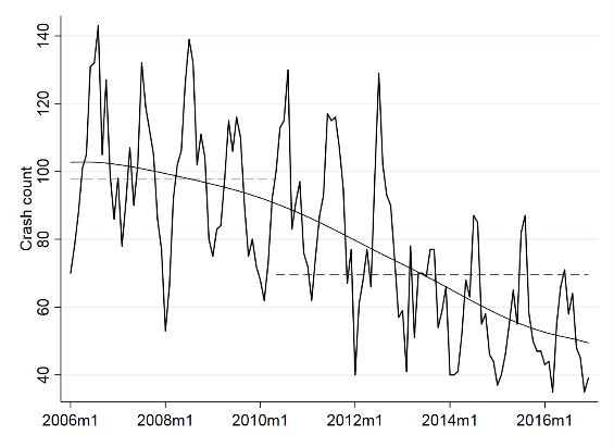
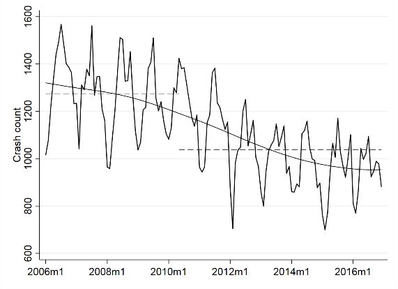
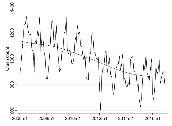
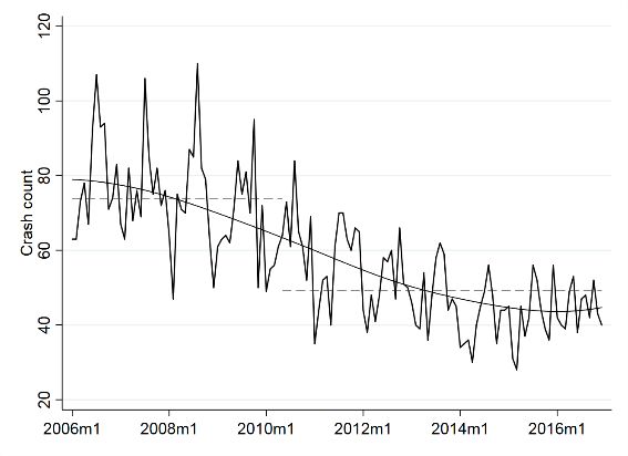
Daylight Savings Time and Car Accidents

preferred bandwidth from Table 3). In Figure A9 we reproduce the mean residuals

plotted in Figure A4. The discontinuous jump for serious accidents is confirmed, over

the first 5 days and then they evolve smoothly over the remaining period, however,

this provides further evidence favouring the ambient light explanation of our results.

We do not test for a sleep deprivation effect for minor accidents when exiting DST

because the Fall transition is not subject to less sleep. Empirical evidence has shown

that people gain some extra minutes of sleep although in a not statistically significant
way (Barnes and Wagner, 2009; Sexton and Beatty, 2014).

4.4 Crash factors

Previous results indicated that ambient light conditions are associated with reduced

vehicle accident counts. However, there can also be other factors affecting the

likelihood of a vehicle accident. Our data do not allow us to identify accidents where
drowsiness is reported as crash factor as in the US paper (Smith, 2016), although

drowsiness is more related to a sleep deprivation mechanism that does not seem to

apply here. However, we can test for whether there is a discontinuous jump in counts

of accidents characterised by bad weather conditions, drunk driving (measured at the

accident scene or post-mortem for fatal crashes), whether they took place in residential

or non-residential areas. An interesting feature of our dataset is that it covers a period

of high economic turbulence. We also split the estimation sample according to the

prevailing economic conditions to examine whether these may exert some influence

on the results. If the economic turmoil during the Greek crisis resulted in a changing

driving behaviour, this could be reflected on the relationship between vehicle crashes

and transitions into and out of DST. There is already evidence that vehicle accidents

mortality has been considerably decreased in Greece during the crisis (Laliotis et al.,

2016; Laliotis and Stavropoulou, 2018). Reduced exposure in the amount of driving for

work and leisure, and adoption of less risky behaviours like smoking, drinking and

speeding during economic downturns have been shown to explain procyclical vehicle-

related fatality (He, 2016; Ruhm, 2000). As seen in Figure A10, all crash counts decline

and become less volatile over time. Although recent empirical analyses place the onset

 18

Ioannis Laliotis, Guiseppe Moscelli & Vassilis Monastiriotis

of the Greek crisis at the end of 2008, when the unemployment rate started to rise, we

use the adoption of the austerity agenda in May 2010 (First Economic Adjustment

Programme) in order to have more balanced samples before and after. Compared to

the period before the crisis, there were 235 less total crashes every month, on average,

and 28 less serious ones during the austerity period.

Table 5 reports the RD estimates accounting for the heterogeneity of DST transitions

by crash factor, type of area and period. Regarding weather conditions, bad weather
seems to be associated with the increase in minor accidents observed during the Fall

transition. For the Spring transition there is a negative, but not significant, effect on

serious accidents, and a significant drop of minor accidents that may seem unexpected

as weather conditions are generally improving during that time of the year. However,
this could simply imply that better ambient light conditions brought by DST mitigate

the effects of adverse driving conditions due to bad weather, especially for minor

accidents – where indeed we should expect the mitigation effect to be stronger/more

effective. Drunk driving (column 2) is related to vehicle accidents during transitions
in a conflicting way. Minor accidents are reduced during the Spring transition and

increase when adopting back the Standard Time. This could reflect the fact that people

are more likely to drink when light conditions deteriorate while devoting more time

to leisure and outdoor activities when gaining one extra hour of sunlight in the Spring.

At the same time fatal and serious accidents where drunk driving is mentioned as a

factor decrease during the Fall transition.

The baseline spring transition effects are primarily driven by accidents taking place in

residential areas (column 3). These results should be expected given the higher traffic
volume in more densely populated locations. Minor accidents decrease during the

Spring transition in non-residential areas as well. This could also be in line with the

ambient light mechanism, as those areas are more affected by the sunlight reallocation

within the day. According to the data, the vast majority, 63.2%, of accidents in non-
residential areas take place in locations with inadequate or inexistent street light.

Finally, baseline effects seem to be driven by changes occurring before the financial

19

Daylight Savings Time and Car Accidents

austerity period. This could be an indication for smaller exposure to the amount of

driving during the crisis and the adoption of less risky driving behaviours, e.g.

smoking, drinking and speeding. It could also be an indication of a substitution effect

towards cheaper means of transportation, e.g. cycling, walking, use of public transport

and car-pooling, when economic conditions deteriorate.

4.5 Omitted variables

In order to test the validity of the adopted RD design, we test for discontinuities of

other factors that can affect driving behaviour. Fuel prices could be considered as such.
Therefore, evidence that fuel prices are smooth at the cutoff should provide

reassurance regarding the estimated effects of the DST policy. We apply the same

estimation strategy using the two most popular fuel products: petrol (unleaded 95

octane) and diesel. According to the European Automobile Manufacturers
Association, 91.7% of the vehicle fleet in Greece was using petrol and 4.9% was using

diesel in 2015, with the remaining vehicles using some alternative fuels. We obtained

daily data from the Fuel Price Observatory of the Ministry of Economy and

Development, regarding the national average prices for these two products. The data

series cover the period between 01 January 2012 and 31 December 2016 (earlier time

series were not available). We regressed the logged fuel prices on the usual set of time

fixed effects and tested for any discontinuous jumps when entering or exiting DST.

Table 6 displays the results. The estimated RD coefficients are quite close to zero

suggesting that fuel prices evolve smoothly during transitions into and out of Summer

Time.

 20

Ioannis Laliotis, Guiseppe Moscelli & Vassilis Monastiriotis

Table 6. RD estimates on the impact of DST transitions on fuel prices.

 Spring transition Fall transition

 Petrol Diesel Petrol Diesel
 (1) (2) (3) (4)

RD estimate -.002 (.009) -.001 (.011) -.002 (.012) -.001 (.016)

Kernel Uniform Uniform Uniform Uniform

Days around transition 16 21 12 13
Source: Ministry of Economy & Development; General Secretariat of Commerce and Consumer Protection;
Fuel Prices Observatory. Authors’ calculations.

Notes: Data cover the period between 01 January 2012 and 31 December 2016 (older series were not
available). The dependent variable is daily price for each fuel product on a set of day-of-week, year and
public holiday fixed effects. Standard errors in parentheses are clustered by day from transition. Asterisks
***, ** and * denote statistical significance at the 1%, 5% and 10% level, respectively.

Another factor related to vehicle accident counts is the amount of driving. It could be

argued that exposure to driving adjusts to the supply of daylight, at least for certain
time intervals within the day. For example, people might drive more for leisure when

the extra hour of sunlight is allocated in the evening after the Spring transition, and

drive less during the respective time interval when falling back to Standard Time.

Smith (2016) tests for such behavioural changes at the Spring transition using vehicle

miles travelled (VMT) data for major highways in California due to the absence of

appropriate data series at the national level. He found no evidence of a statistically

significant discontinuity at the Spring cutoff. We are also constrained by the lack of

national daily time series on road usage. The only available data were those provided

by the Observatory Unit of the Egnatia Road, a major highway network on northern

Greece and part of the European E90 highway system. For a large part of their

network, Egnatia Road S.A. provided daily time series on road usage, in terms of

number of vehicles passing through toll stations, covering the period between 01

January 2012 and 31 December 2016. However, no significant discontinuities were

uncovered at the transition dates. The estimated RD parameters for the Spring and Fall

transitions were 0.054 (standard error 0.035) and 0.012 (standard error 0.043),

respectively, both of them being not statistically significant.

21

Daylight Savings Time and Car Accidents

4.6 Implications

The estimated effects of DST on vehicle accident counts may have serious implications

on health, healthcare and other services utilisation, productivity and foregone hours

of work and personal time. Hence, the exact evaluation of the overall impact is
difficult. However, we attempt some back-of-the-envelope calculations in order to

quantify the estimated baseline impacts of DST transitions in terms of vehicle

insurance claims. For this reason, we use information extracted from the Statistical

Yearbooks for Motor Insurance published by the Hellenic Association of Insurance
Companies (HAIC). Those reports are available online for the period after 2010. This

enables us to compute the number of the total insurance claims costs that could be

spared in the absence of the DST policy.

We start by performing this exercise for the case of minor accidents when leaving DST,
because the quantification of the costs implied by more serious crashes is relatively

more difficult as it incorporates costs that cannot be reliably measured and also

because the baseline Spring transition impact on minor accidents was not statistically

significant. In order to consider only minor accidents, we used vehicle insurance

claims, excluding those related to fire and theft, supposing a maximum settlement

amount of 2,000 euros. Because the HAIC Yearbooks report the annual number of

claims, we multiplied those figures with 14/365, i.e. using the number of days

suggested by the bandwidth choice. The results are presented in Table 7. The number

of total claims net of those related to fire and theft, in column 4, is multiplied by 1 −

2 < − 15, where b is the baseline effect for minor accidents in Table 3. According to the

results there would be 2,082 fewer claims worth up to 2,000 euros for motor accidents

each year, on average. Multiplying the annual claims differences (column 6) by the
total amount of settlements for insurance claims worth up to 2,000 euros implies an

average extra cost of nearly 1.45 million euros each year. Of course, these results are

determined by the use of the total period DST impact, incorporating both periods

before and during the crisis. Using the post-2010 estimate, i.e. b = 0.037 but not

statistically significant (column 6 in Table 5; panel B), in order to match exactly with

 22

Ioannis Laliotis, Guiseppe Moscelli & Vassilis Monastiriotis

the period covered by the HAIC Statistical Yearbooks suggests that there would be

nearly 638 extra claims for minor vehicle damages due to leaving DST, inducing extra

costs of about 445 thousand euros per year, on average.

Similar back-of-the-envelope calculations using the baseline for serious accidents

during the Spring transitions (using the baseline estimate in Table 3, i.e. -0.253) can be

performed although it is difficult to assume the settlement amount for a serious, non-

fatal crash. Assuming settlements between 2,001 euros and 50,000 euros (and an 18-
day bandwidth), suggests that entering DST is associated with nearly 4.8 thousand

fewer claims each year, hence generating annual cost savings of about 10.3 million

euros, on average.8 Combining the insurance claims implications for serious accidents

when entering DST and minor accidents when leaving DST implies an average cost
reduction of about 8.8 million euros per year from adopting/not abolishing a DST

policy.

However, these are conservative and lower bound estimates of the costs to be spared.

Passengers involved even in minor traffic accidents are likely to visit hospitals to check
their health status, forgo hours of work due to the accident, engage in administrative

procedures to cope with insurance reimbursements, and suffer post-traumatic stress.

These events respectively imply healthcare costs to be sustained by the individual

and/or the state, forgone earnings due to absence from work, increased vehicle

insurance premia, payment of charges for driver misconduct, and monetary and non-

monetary expenses related to mental health distress, e.g. decrease in productivity,

greater anxiety etc. Lack of reliable data on these events restricts us from a proper

quantification of the overall costs faced by individuals involved into vehicle accidents.

8 Full results for insurance claims implications of serious accidents are available upon request.

23

Daylight Savings Time and Car Accidents

 Table 7. Estimates of insurance claims costs for minor accidents due to DST.

 Total Theft Fire Actual net Net total Differenc Estimated total
 Year
 number of claims claims total claims claims e due to cost (€) due to
 declared without DST DST
 claims DST
 (1) (2) (3) (4) (5) (6) (7)

 2010 21,784 469 39 21,277 18,660 2,617 1,722,477

 2011 20,197 525 37 19,636 17,221 2,415 1,590,423

 2012 16,697 482 31 16,185 14,195 1,991 1,417,353

 2013 15,737 389 24 15,324 13,439 1,885 1,391,358

 2014 15,679 346 17 15,317 13,433 1,884 1,376,507

 2015 15,481 359 18 15,104 13,246 1,858 1,359,461

 2016 16,079 382 21 15,677 13,749 1,928 1,310,138

 Source: Statistical Yearbook for Motor Insurance, 2010-2013 (Hellenic Association of Insurance
 Companies).

 Notes: Column (5) is the counterfactual number of total claims in the absence of DST, computed as:
 Actual Net Total Claims×[1-(exp(0.116)-1)], where 0.116 is the baseline estimate for minor crashes
 during the fall transition date. Column (7) is column (6) multiplied by the total amount of settlements
 for insurance claims worth up to €2,000.

However, these are conservative and lower bound estimates of the costs to be spared.

Passengers involved even in minor traffic accidents are likely to visit hospitals to check

their health status, forgo hours of work due to the accident, engage in administrative

procedures to cope with insurance reimbursements, and suffer post-traumatic stress.

These events respectively imply healthcare costs to be sustained by the individual

and/or the state, forgone earnings due to absence from work, increased vehicle

insurance premia, payment of charges for driver misconduct, and monetary and non-
monetary expenses related to mental health distress, e.g. decrease in productivity,

greater anxiety etc. Lack of reliable data on these events restricts us from a proper

quantification of the overall costs faced by individuals involved into vehicle accidents.

 24