Cross-species behavior analysis with attentionbased domain-adversarial deep neural networks
←
→
Page content transcription
If your browser does not render page correctly, please read the page content below
ARTICLE
                  https://doi.org/10.1038/s41467-021-25636-x                 OPEN

                  Cross-species behavior analysis with attention-
                  based domain-adversarial deep neural networks
                  Takuya Maekawa              1 ✉,   Daiki Higashide1, Takahiro Hara1, Kentarou Matsumura2, Kaoru Ide3,
                  Takahisa Miyatake             4,   Koutarou D. Kimura 5 & Susumu Takahashi3
1234567890():,;

                  Since the variables inherent to various diseases cannot be controlled directly in humans,
                  behavioral dysfunctions have been examined in model organisms, leading to better under-
                  standing their underlying mechanisms. However, because the spatial and temporal scales of
                  animal locomotion vary widely among species, conventional statistical analyses cannot be
                  used to discover knowledge from the locomotion data. We propose a procedure to auto-
                  matically discover locomotion features shared among animal species by means of domain-
                  adversarial deep neural networks. Our neural network is equipped with a function which
                  explains the meaning of segments of locomotion where the cross-species features are hidden
                  by incorporating an attention mechanism into the neural network, regarded as a black box. It
                  enables us to formulate a human-interpretable rule about the cross-species locomotion
                  feature and validate it using statistical tests. We demonstrate the versatility of this procedure
                  by identifying locomotion features shared across different species with dopamine deficiency,
                  namely humans, mice, and worms, despite their evolutionary differences.

                  1 Graduate School of Information Science and Technology, Osaka University, Osaka, Japan. 2 Graduate School of Agriculture, Kagawa University,

                  Kagawa, Japan. 3 Graduate School of Brain Science, Doshisha University, Kyoto, Japan. 4 Graduate School of Environmental and Life Science, Okayama
                  University, Okayama, Japan. 5 Graduate School of Science, Nagoya City University, Aichi, Japan. ✉email: maekawa@ist.osaka-u.ac.jp

                  NATURE COMMUNICATIONS | (2021)12:5519 | https://doi.org/10.1038/s41467-021-25636-x | www.nature.com/naturecommunications                             1
ARTICLE                                                                 NATURE COMMUNICATIONS | https://doi.org/10.1038/s41467-021-25636-x

N
        eurodegenerative diseases including Parkinson’s disease                To demonstrate the performance of our proposed cross-species
        (PD), Alzheimer’s disease, and schizophrenia are dis-                behavioral analysis, we identified locomotion features shared
        orders characterized by motor dysfunctions. Since the                across different species with dopamine deficiency, namely
variables inherent to such diseases cannot be controlled directly            humans, mice, and worms.
in humans, behavioral dysfunctions and their neural under-
pinnings have been examined in model organisms1,2. Assuming                  Results
that fundamental aspects of the behavior of humans are evolu-                Attention-based domain-adversarial neural network. This study
tionarily conserved among other animal species, studies in model             assumes that locomotion data from two different species that
organisms gained insights into understanding the underlying                  belong to two different classes, for example, PD individuals and
mechanisms of those diseases3–6. In contrast to cognitive                    healthy individuals of humans and mice are given. The locomo-
abnormalities, motor dysfunctions can be externally assessed by              tion data are used to train the neural network (see Fig. 1d). The
comparative behavioral analyses. A central concept of compara-               model inputs are time-series of primitive locomotion features
tive behavioral analysis is to identify human-like behavioral                such as speed. The model has two types of outputs: estimated
repertoires, called behavioral phenotype, in animals, as animal              domain and class of an input time-series.
models of PD have gained insight into understanding the beha-                   The convolutional layers in the feature extraction block are
vioral and neural underpinning of symptoms underlying a spe-                 used to extract features, which are used to output the two
cific disease7 and can potentially provide clues for the                      estimates. We introduce the gradient reversal layer8 before the 1st
development of therapeutics. However, behavioral analysis across             domain predictor. When we train the network using the
animal species could not be realized using conventional statistical          backpropagation algorithm11, the gradient reversal layer multi-
analyses because the body scale and locomotion methods vary                  plies the gradient with a negative constant value, making the
among species (Fig. 1a), resulting in wide variations in the spatial         convolutional layers in the feature extraction block incapable of
and temporal scales of locomotion among species as shown in                  estimating domains but classes.
Fig. 1b in which worms, beetles, and mice show similar loco-                    In addition, we introduce an attention mechanism9 into the
motion trajectory, but differ in the velocity and spatial area               model. The attention of a data point at each time slice is regarded
occupied.                                                                    as the importance of the data point when the input time-series is
   Deep learning is a novel technique of automated feature                   classified, indicating that attended data points are characteristic to
extraction, reducing the cost of manual feature design. We                   a class to which the input time-series belongs. The convolutional
employ it for automatically discovering scale-invariant locomo-              layers in the attention computation block are used to compute
tion features shared among animal species. In the procedure (see             attention for each time slice. The attention is multiplied by
Fig. 1c), a human operator first feeds locomotion data from                   the extracted features to contrast the data points to which the
animals of different species with different properties into a neural         network pays attention. Furthermore, to make the way of
network designed to extract cross-species locomotion features                attention computation domain-independent, we introduce the
using domain-adversarial training8. This is trained to extract               gradient reversal layer after the 2nd convolutional layer in the
features that classify a trajectory into an appropriate class (e.g.,         attention computation block. The 2nd domain predictor outputs
healthy or PD) but cannot label the trajectory into an appropriate           domain estimate for each time slice using the output of the 2nd
domain (i.e., species), using a gradient reversal layer as shown in          convolutional layer in the attention computation block and we
Fig. 1d. Because these features are incapable of distinguishing              make the network incapable of classifying the output of the 2nd
between domains, we can regard them as species-independent. In               convolutional layer into domains using the gradient
contrast, because we can distinguish between trajectories                    reversal layer.
belonging to different classes using the extracted features, these              Here we briefly explain the difference between the network and
can be regarded as cross-species hallmarks of the diseases. By               that proposed in DeepHL (DeepHL-Net)12, which is our prior
designing a deep neural network so that it extracts features based           work. Because DeepHL-Net is trained on trajectories from a
on the above idea, we can obtain locomotion features shared                  single species, DeepHL-Net outputs only a class estimate, for
across different species independent of their body scales and                instance, healthy or PD class. Therefore, DeepHL-Net relies
locomotion methods.                                                          mainly on attention mechanisms that detect segments character-
   Despite the human-level outstanding performances of the                   istic of a class. In contrast, in this study, the network is trained on
neural network, the human operator cannot understand the                     trajectories from two species, and outputs domain and class
meaning of the extracted cross-species locomotion feature by                 estimates. To render the network incapable of distinguishing
the deep neural network containing a huge amount of hidden                   between the two domains, we introduce domain-adversarial
parameters. To address this issue, we design an explainable                  training (gradient reversal). More specifically, gradient reversal is
architecture by incorporating an attention mechanism9,10 into the            introduced to render the ways of feature extraction and attention
domain-adversarial neural network, which identifies segments in               computation domain-independent.
the trajectories where the cross-species features are hidden and                The network is trained to minimize the error of the class
provides visualized trajectories and time-series of basic locomo-            estimates as well as maximize the errors of the two types of
tion features (e.g., speed) by highlighting the identified segments           domain estimates. However, achieving these conflicting goals at
(Fig. 1e, f). From these highlighted graphs, the operator can                the same time makes it difficult for the neural network to
understand cross-species locomotion features extracted by the                converge. Therefore, we iterate the following procedures to train
neural network. For instance, short-duration peaks in speed are              the network.
characteristic to PD mice (Fig. 1f). To explain why the neural
network pays attention to a certain segment and how it labels an                1. We first train the network to minimize the error of the class
input time-series using attended segments within the time-series,                  estimates as well as maximize the error of the domain
we employ decision trees. They help formulate a human-                             estimates by the 2nd domain predictor, which employs
interpretable rule about the cross-species locomotion feature.                     outputs of the attention computation block to predict the
Then, the operator proposes a hypothesis related to the loco-                      domain. Thus we extract important segments in the input
motion features and performs a statistical test to validate it (see                time-series for class estimation in a domain-independent
Fig. 1c).                                                                          manner.

2                NATURE COMMUNICATIONS | (2021)12:5519 | https://doi.org/10.1038/s41467-021-25636-x | www.nature.com/naturecommunications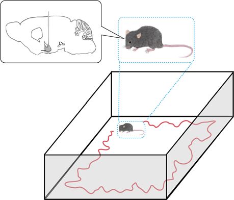
NATURE COMMUNICATIONS | https://doi.org/10.1038/s41467-021-25636-x ARTICLE
a
Mouse
Beetle
Worm Human
10-1 100 101 102 103 104 (mm)
b c
1 cm 1 cm Deep learning-assisted
knowledge discovery
Human-
interpret
able rule
10 cm 10 cm
Animals with
Normal animals Validation
dopamine-deficient
(statistical test)
Input time-series e
d
Attention computation block
extraction block
1D Conv & 1D Conv &
Feature
Dropout Dropout
1D Conv & 1D Conv &
Dropout Dropout
Attention
Normal mouse PD mouse
time steps
Gradient Gradient
f
Dense
reversal reversal
Dense Dense Dense
Class estimate
Dense Dense
2nd Domain estimate 1st Domain estimate
Normal mouse speed PD mouse speed
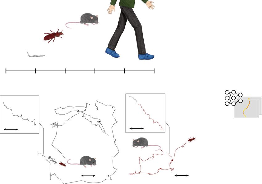
Fig. 1 Cross-species behavior analysis using a domain-adversarial neural network with attention mechanism. a Differences in body scales among
different species. b Locomotion trajectories of different animals (worm, beetle, and mouse) differ at the spatial scale, but show similar patterns, left, black
lines depict locomotion trajectories of normal animals, right, red lines show trajectories of dopamine-deficient individuals, inset, expanded trajectories of
worms. c Our proposed procedure automatically finds a locomotion feature shared by different animals using deep learning, and exhibits the learned
locomotion features, enabling the human operator to extract a hypothesis and validate the statistical significance. d Proposed network architecture: the
feature extraction block learns feature representation that maximizes class prediction accuracy but minimizes domain prediction accuracy by using a
gradient reversal layer; the learned feature is assumed to be domain-independent because the feature is incapable of distinguishing between the domains,
while the attention computation block computes an attention value for each time slice in a domain-independent manner by using a gradient reversal layer. e
Highlighted trajectories of normal and Parkinson’s disease (PD) mice by attention values of the neural network that is trained to extract cross-species
locomotion features of worms and mice. f Example time-series of the speed of normal/PD mice highlighted by our network, where the attention level is
color-coded according to the scale bar shown on the right.
NATURE COMMUNICATIONS | (2021)12:5519 | https://doi.org/10.1038/s41467-021-25636-x | www.nature.com/naturecommunications 3ARTICLE NATURE COMMUNICATIONS | https://doi.org/10.1038/s41467-021-25636-x
2. Then we update the network to maximize the error of Figure 2f shows a decision tree trained to detect the attended
domain estimates by the 1st domain predictor to accelerate segments. The root node and its right child node indicate that
training in the next procedure. attended segments correspond to segments with long-lasting high
3. Finally, we update the network to minimize the error of speed. (High minimum speed in a sliding window, i.e., a high
class estimates as well as maximize the error of domain moving minimum of speed, indicates keeping high speed.) Fig. 2g
estimates by the 1st domain predictor. With this procedure, shows a decision tree trained to classify an input time-series into
we can train the network to predict class labels correctly but an appropriate class using features extracted from attended
domain labels incorrectly. segments within the time-series. As shown in the root node and
See Methods for more details about the procedures. Fig. 2f, the neural network seems to pay attention to the long-
In addition, to help understand the meaning of attention, we lasting high speed of the worms/mice using the attention
employ machine learning tools to explain it. We construct a mechanism, and then distinguishes between DA(+) and DA(−)
decision tree that is trained to detect the attended segments by the by the skewness of speed within the attended segments. The
neural network using exhaustively handcrafted features listed in attended segments with positive skewness (≥0.360) are classified
Supplementary Table 1. into the DA(−) class. In contrast, the attended segments with
Furthermore, to interpret how the neural network predicts skewness smaller than 0.360 are classified into the DA(+) class
classes using attended segments, we build a decision tree that is (between −0.397 and 0.360). Therefore, these results indicate that
trained to classify an input time-series using handcrafted features the DA(+) worm/mouse keeps stable speed (small skewness)
extracted only from attended segments within the time-series. See when moving at high speed.
Methods for more details. As above, we could extract an interpretable rule from the
As above, an interpretable rule is extracted from our neural trained neural network, i.e., DA(−) worms/mice cannot keep
network with the explainable architecture and/or by our methods high speed. To validate the hypothesis, we perform a statistical
based on decision trees. After that, the interpretable rule is test by computing the minimum speed within a time window
investigated via a statistical test. To validate our procedure, we when the speed is high (see Supplementary Information for
prepared locomotion data from four different dopamine-deficient details). As shown in Fig. 2h, we observe significant differences
species (humans, mice, beetles, and worms). We train our neural between DA(+) and DA(−) for both the mice and worms.
network on data from two species to obtain an interpretable rule Surprisingly, we could also observe significant differences
and then validate this using data from all the species. We only between PD and healthy humans when we performed the same
use data from two species because doing otherwise would increase test, even though the neural network was trained only on the data
the complexity of the classification task, making it difficult for from the mice and worms. See Methods for details about the
the network to converge. human data.
We have made the codes for our deep learning method and As above, our method revealed that humans, mice, and worms
decision tree construction available as Supplementary Software 1. with disabilities in the dopaminergic system cannot keep high
speed even though their body scales and locomotion methods are
completely different. Our study employs worms with a lack of D2
dopamine receptors. Although the PD symptoms are considered
Network training on worm and mouse data. We use locomotion to be induced by various impairment of neural circuits such as
data from worms with/without DOP-3, one of the D2 dopamine dopamine transmission impairment, morphological alterations of
receptors13, and from healthy and PD mice. A PD mouse is a
the basal ganglia circuitry, and lack of dopamine receptors16–19, a
unilateral 6-hydroxydopamine (OHDA) lesioned model of PD major source of the discovered locomotion feature shared by PD
whose dopaminergic neurons in the compact part of substantia
mice and humans might ascribe the lack of D2 dopamine
nigra of a left or right hemisphere are lesioned with a neurotoxin receptors. The verification of this hypothesis is beyond the scope
6-OHDA. Fig. 2a, b show the data collection protocols. Prior
of this study.
studies discovered relevant locomotion features of PD mice1,2 as
well as of worms during odor avoidance behavior14,15. However,
locomotion features across these species have not been investi- Network Training on Worm and Human Data. Next, we show
gated because the scales of their movements are significantly
results obtained when the neural network is trained on data from
different. We convert 2D locomotion data from worms and mice worms and humans. As for the human data (see Methods and
into time-series of locomotion speed and then standardize each
Supplementary Table 2), we convert time-series of foot-mounted
time-series to normalize the range of the variables. Note that pressure sensors collected during walking into time-series of
because the lengths of the time-series of the speed of worms differ
locomotion speed.
from those of mice, we have undersampled the time-series from We deal with two classes, i.e., DA(+) class (healthy worms and
the mice so that the lengths of the time-series are identical to
humans) vs. DA(−) class (PD humans and worms lacking D2
those from the worms. More details about the data are available dopamine receptors). Fig. 3a, b shows the classification accuracy,
in Methods and Supplementary Table 2.
indicating that our network seems to extract a cross-species
We randomly split the speed time-series data into training and feature between humans and worms. Fig. 3c shows the time-series
test sets, which are fed into the neural network. We deal with two
of speed for DA(+)/DA(−) worms and humans highlighted by
classes, DA(+) class (healthy mice and worms) vs. DA(−) class the trained model. From these highlighted time-series, the neural
(PD mice and worms lacking D2 dopamine receptors), and two
network seems to focus on segments corresponding to smooth
domains (mouse and worm). The classification accuracy is shown acceleration for the DA(+) worms and humans. (A decision tree
in Fig. 2c, d, indicating that our network cannot distinguish the
shown below also takes an acceleration feature as a root node.)
domains but the classes. These results indicate that cross-species Fig. 3d shows the time-series of acceleration for worms and
features of DA(−) among mice and worms exist. Fig. 2e shows an
humans, as segments of DA(+) worms/humans corresponding to
example of time-series of speed for worms and mice highlighted acceleration are attended.
by the trained model. From these highlighted time-series, we can
Figure 3e shows a decision tree that is trained to detect the
speculate that the neural network focuses on segments corre- attended segments. The root node and its right child node indicate
sponding to high speed for the DA(+) worms and mice.
that attended segments correspond to segments with high
4 NATURE COMMUNICATIONS | (2021)12:5519 | https://doi.org/10.1038/s41467-021-25636-x | www.nature.com/naturecommunicationsNATURE COMMUNICATIONS | https://doi.org/10.1038/s41467-021-25636-x ARTICLE
6-OHDA
a b (Top view) c
CPu
SNCD
Odor Worm Mouse All
mfb
source Start Train 0.80 0.87 0.84
USB
camera ʹ
Test 0.69 0.81 0.75
ʹ
ʹ
d Domain 1 Domain 2
60 cm Train 0.54 0.54
20 cm
Test 0.50 0.53
1 cm
55 cm
e
DA(+) mouse speed DA(-) mouse speed DA(+) worm speed DA(-) worm speed
f g
DA(-)
DA(+)
h
0.20
0.50
Normalized minimum speed
0.80
0.60
0.30
0.10
0.20 0.40
0.10
0.00
DA(+) mouse DA(-) mouse DA(+) worm DA(-) worm DA(+) human DA(-) human
Fig. 2 Analysis of DA(+)/DA(−) mice and worms (DA: dopamine). a A Parkinson’s disease (PD) mouse walks in the experimental setup, where
dopaminergic neurons in the substantia nigra pars compacta were unilaterally lesioned with 6-hydroxydopamine. b The experimental setup (left) for
monitoring the worm’s trajectory (right). c Classification accuracies of our network for DA(+)/DA(−) classes. d Classification accuracies of our network
for the 1st and 2nd domain estimates, where the random guess ratio is 0.5 (1/2); see Supplementary Information for the detailed results of the domain
estimates. e Example time-series of speed of DA(+)/DA(−) mice and worms highlighted by our network. f A decision tree for explaining the meaning of
attention by the neural network, i.e., classifying attended (`attention') and non-attended (`none') segments, where features were normalized for each
trajectory (min–max normalization); we show only the 1st and 2nd layers and each histogram shows a tree node of the tree, and a feature used in the node
is indicated at the bottom of the histogram; a histogram of each node is constructed from training instances' values of a feature used in the node, instances
having feature values smaller than a threshold go to the left child, the threshold value is shown at the bottom of each histogram associated with a black
arrow and pie charts at the bottom of the tree (leaf nodes) show distributions of training instances classified by the tree. g A decision tree for explaining
classification, where we show only the 1st layer. h Distributions of averaged minimum speed within a time window when the speed is high for mice/worms;
to compute the averaged minimum speed, we compute the rolling minimum of the normalized speed within segments with high speed (top 20% average
speed) for each trajectory (see Supplementary Information for details) and the box plot shows the 25–75% quartile, with embedded bar representing the
median and the lower/upper whiskers show Q1-1.5*IQR and Q3+1.5*IQR, respectively, where IQR is the interquartile range, Q1 is 25% quartile, and Q3 is
75% quartile; significant differences between DA(+) and DA(−) for both the mice and worms are observed (worm by the Brunner–Munzel test:
p = 7.61 × 10⁻⁴: w = 3.48; df = 90.41; effectsize = 0.65; n = 162 from DA(+) worms; n = 47 from DA(−) worms; mouse by the Welch’s t-test:
p = 2.53 × 10⁻³; t = 3.07; df = 131.45; effectsize(r) = 0.45; n = 88 10 min trajectories from DA(+) mice; n = 113 10 min trajectories from DA(−) mice); a
significant difference between DA(+) and DA(−) for the humans is also observed by the Welch’s t-test (p = 0.03; t = 2.25; df = 123.83;
effectsize(r) = − 0.32; n = 78 from DA(+) humans; n = 163 from DA(−) humans); the p value is two sided; see Supplementary Information for the
normality tests of the distributions, which were used to select methods of statistical test for comparing two groups.
acceleration values as well as high minimum speed values within a appropriate class using features extracted from attended segments
time window. This result indicates that the neural network focuses within the time-series. As shown in the root node and Fig. 3e, the
on a moment of long-lasting acceleration. Fig. 3f shows a decision neural network seems to pay attention to long-lasting accelerations
tree that is trained to classify an input time-series into an of the DA(+) worms/humans using the attention mechanism, and
NATURE COMMUNICATIONS | (2021)12:5519 | https://doi.org/10.1038/s41467-021-25636-x | www.nature.com/naturecommunications 5ARTICLE NATURE COMMUNICATIONS | https://doi.org/10.1038/s41467-021-25636-x
a e
Worm Human All
Train 0.92 0.92 0.92
Test 0.81 0.88 0.85
b Domain 1 Domain 2
Train 0.54 0.52
Test 0.34 0.51
c
DA(+) human speed DA(-) human speed
f
DA(+) worm speed DA(-)
DOP
DA(-) worm speed
DA(+)
d
DA(+) human ACC. DA(-) human ACC.
g
Normalized minimum speed
0.7 0.14
0.25
0.6 0.12
0.5 0.20 0.10
DA(+) worm ACC. DA(-) worm ACC. 0.4 0.08
0.15
0.06
0.3
0.10 0.04
0.2
0.02
0.1 0.05 0.00
DA(+) human DA(-) human DA(+) worm DA(-) worm DA(+) mouse DA(-) mouse
Fig. 3 Analysis of DA(+)/DA(−) humans and worms (DA: dopamine). a Classification accuracies of our network for DA(+)/DA(−) classes. b
Classification accuracies of our network for the 1st and 2nd domain estimates; see Supplementary Information for the detailed results of the domain
estimates. c Example time-series of the speed of DA(+)/DA(−) humans and worms highlighted by our network. d Example time-series of acceleration of
DA(+)/DA(−) humans and worms highlighted by our network. e A decision tree for explaining the meaning of attention. f A decision tree for explaining
classification. g Distributions of minimum speed within a time window when the average acceleration is high for humans and worms (see Supplementary
Information for details); significant differences between DA(+) and DA(−) for both humans and worms are observed (worm by the Brunner–Munzel test:
p = 0.03; w = 2.26; df = 101.91; effectsize = 0.60; n = 162 from DA(+) worms; n = 47 from DA(−) worms; human by the Welch’s t-test: p = 0.02;
t = −2.35; df = 126.89; effectsize(r) = −0.34; n = 78 from DA(+) humans; n = 163 from DA(−) humans); a significant difference between DA(+) and
DA(−) for the mice is also observed by the Welch’s t-test (p = 0, 01; t = 2.57; df = 131.63; effectsize(r) = 0.38); n = 88 10 min trajectories from DA(+)
mice; n = 113 10 min trajectories from DA(-) mice; the p-value is two sided. The box plot shows the 25–75% quartile, with an embedded bar representing
the median and the lower/upper whiskers show Q1-1.5*IQR and Q3+1.5*IQR, respectively, where IQR is the interquartile range, Q1 is 25% quartile, and Q3
is 75% quartile.
then distinguishes between DA(+) and DA(−) simply by the when the average acceleration is high (see Supplementary
minimum of speed within the attended segments. Information for details). As shown in Fig. 3g, we observe
From the above results, we can say that the DA(−) worms/ significant differences between DA(+) and DA(−) for both
humans present unstable speed while accelerating (lower humans and worms. Interestingly, we could also observe
minimum speed during high acceleration). To validate the significant differences between the two classes of mice.
hypothesis, we perform a statistical test. Based on the decision As above, we could notice that the speed of these animals is
trees, we compute the minimum speed within a time window unstable when accelerating. PD mice used in this study (6-OHDA
6 NATURE COMMUNICATIONS | (2021)12:5519 | https://doi.org/10.1038/s41467-021-25636-x | www.nature.com/naturecommunicationsNATURE COMMUNICATIONS | https://doi.org/10.1038/s41467-021-25636-x ARTICLE
a b Worm Beetle All
Train 0.98 0.83 0.91
Test 0.81 0.81 0.81
c Domain 1 Domain 2
Train 0.58 0.50
Test 0.60 0.50
Start
d e
Start
DA(+) beetle DA(-) beetle DA(+) beetle speed DA(-) beetle speed
Start Start
DA(+) worm DA(-) worm DA(+) worm speed DA(-) worm speed
f 1.5
Normalized moving
acceleration
1.0
0.5
0.0
-0.5
DA(+) beetle DA(-) beetle DA(+) worm DA(-) worm DA(+) mouse DA(-) mouse
Fig. 4 Analysis of DA(+)/DA(−) beetles and worms. (DA: dopamine). a Experimental apparatus for beetle study (treadmill). b Classification accuracies
of our network for DA(+)/DA(−) classes. c Classification accuracies of our network for the 1st and 2nd domain estimates; see Supplementary Information
for the detailed results of the domain estimates. d Example trajectories of DA(+)/DA(−) beetles and worms highlighted by our network. e Example time-
series of speed of DA(+)/DA(−) beetles and worms highlighted by our network. f Distributions of acceleration before turns for beetles and worms
(see Supplementary Information for details); significant differences between DA(+) and DA(−) for both beetles and worms are observed (worm by the
Brunner–Munzel test: p = 0.005; w = − 2.90; df = 72.76; effectsize = 0.36; n = 162 from DA(+) worms; n = 47 from DA(−) worms; beetle by the
Brunner–Munzel test: p = 2.99 × 10⁻⁸; w = − 6.22; df = 71.50; effectsize = 0.18; n = 40 from DA(+) beetles; n = 40 from DA(−) beetles); a significant
difference between DA(+) and DA(−) for the mice is also observed by the Welch’s t-test (p = 0.02; t = − 2.37; df = 112.94; effectsize(r) = − 0.35);
n = 88 10 min trajectories from DA(+) mice; n = 113 10 min trajectories from DA(−) mice; the p-value is two sided. The box plot shows the 25–75%
quartile, with embedded bar representing the median and the lower/upper whiskers show Q1-1.5*IQR and Q3+1.5*IQR, respectively, where IQR is the
interquartile range, Q1 is 25% quartile, and Q3 is 75% quartile.
mouse model of PD) are considered to exhibit motor symptoms as an anti-predator strategy21. The selection regimes for a short or
of akinesia and bradykinesia20. The discovered locomotion long duration of tonic immobility have been established in the red
feature is similar to the symptom of akinesia. Our study reveals flour beetle, Tribolium castaneum22. We use trajectory data of
that a similar feature is also found in worms lacking D2 dopamine beetles collected from the short and long selection regimes on a
receptors, indicating that the receptors play an important role in treadmill (Fig. 4a; short: 20 beetles; long: 20 beetles). The long
the symptom. selection regime showed significantly lower levels of brain
dopamine expression and lower locomotor activity than those of
the short selection regime23. Further, Uchiyama et al.24 showed
Network training on worm and beetle data. Tonic immobility 518 differentially expressed genes between the selection regimes.
(sometimes called death-feigning behavior or thanatosis) has As expected from physiological studies described above, genes
been observed in many species and it is thought to have evolved associated with the metabolic pathways of tyrosine, a precursor of
NATURE COMMUNICATIONS | (2021)12:5519 | https://doi.org/10.1038/s41467-021-25636-x | www.nature.com/naturecommunications 7ARTICLE NATURE COMMUNICATIONS | https://doi.org/10.1038/s41467-021-25636-x
dopamine, were differentially expressed between the short and To demonstrate the usefulness of the proposed neural network,
long selection regime; these enzyme-encoding genes were we found cross-species locomotion features among species that
expressed at higher levels in the long selection regime than in the are far away from each other in the evolutionary lineage. The
short selection regime24. Therefore, we train the neural network study reveals that the DA(−) humans, mice, and worms cannot
with the long selection regime corresponding to the DA(−) class. keep high speed. In addition, the speed of the DA(−) humans,
Figure 4b, c show the classification accuracy. Fig. 4d shows mice, and worms is unstable when accelerating. Moreover, the
trajectories of DA(+)/DA(−) worms and beetles highlighted by DA(−) worms, mice, and beetles present significantly high
the trained model, indicating that the network focuses on acceleration before they changing direction. We believe that
segments before the movement direction changes in many cases. discovering such hypotheses from time-series trajectory data
Fig. 4e shows the time-series of speed for DA(+)/DA(−) worms obtained from multiple species is difficult. In this study, we
and beetles highlighted by the trained model. As shown in these focused on specific important moments in the time-series high-
figures, the network focuses on segments before the local minima lighted by the attention mechanisms, e.g., moments of accelera-
of speed (corresponding to direction changes, e.g., t = 17, 23 for tion and moments before the turn. However, it is difficult to focus
DA(+) beetle). Before the turns, DA(+) worms and beetles seem on such moments by manually analyzing trajectories from mul-
to quickly decrease their speed. In contrast, DA(−) worms and tiple species.
beetles do not seem to smoothly decrease their speed (e.g., t = 15, While training the neural network using data from two species,
20 for DA(−) beetle). Based on the observation, we compare the the discovered locomotion features from one of them were
difference in acceleration before turns between the DA(+) and observed in other species as well, indicating that the neural net-
DA(−) classes (see Supplementary Information for details). As work captures latent locomotion features across different species.
shown in Fig. 4f, we could observe significant differences between As a result, we propose the hypothesis that various aspects of
DA(+) and DA(−) for both beetles and worms. Yamazaki et al.15 motor dysfunction across animal species can be explained by the
revealed that the dopamine-deficient worms are abnormal in deficiency of dopamine expression levels. Our method could thus
speed changes before the initiation of turns, a result which is in be useful in identifying animal models for a variety of Parkinson’s
keeping with the findings of our study. In addition, recent disease symptoms such as akinesia, bradykinesia, tremor, rigidity,
analysis on DNA sequences of beetles25 revealed that DA(−) and postural instability.
beetles have large mutations in dopamine-related genes compared In practice, researchers may label trajectories mistakenly. For
with DA(+) beetles, suggesting that DA(−) beetles exhibit example, some DA(+) trajectories can be mistakenly labeled as
abnormal walking behaviors compared with DA(+) beetles DA(−). Our additional investigation on the robustness of our
due to changes to the dopaminergic system. We could also method against potential labeling errors revealed that, even when
observe significant differences between the two classes of mice. 5% of erroneous labels are included, our model maintains high
Because we only have speed time-series for the human data, we classification accuracy. See Supplementary Information and
could not perform this test for humans. Supplementary Figure 4 for more detail.
As above, we observed that DA(−) animals exhibit significantly Here we discuss the rationale for using a decision tree in the
high acceleration before they change the moving direction. This process of explaining the meaning of attended segments. The aim
indicates that the animals with dopamine deficiency cannot of this process is to help understand the meaning of the attended
smoothly decrease the speed before turns. Specifically, this segments. It is therefore important to explain the meaning of
hypothesis found by our method focuses on the transition from attention using a small number of features. Even though regres-
the "running” mode to the "turn” mode. The disability in sion models enable us to detect important features highly corre-
locomotion mode transition caused by PD has been studied on lated with the attended segments, the regression models suffer
mice and humans20,26. These lines of evidence suggest that the from multicollinearity. Because some locomotion features–such
disability is caused by combined factors constituting morpholo- as speed and acceleration–are correlated with each other, it is
gical abnormalities of the neural circuitry and changes of the DA difficult to use the regression models in this procedure. Although
transporter and in the DA receptor densities induced by the lack the support vector machine (SVM) is a widely-used classifier and
of DA. On the other hand, our cross-species comparative analysis achieves high classification accuracy, the interpretability of the
proposes a hypothesis that the disability can be simply explained model is poor because the SVM learns a classification rule in a
by the deficiency of dopamine expression level. high-dimensional feature space when many features are available.
Another possible approach is to use a method for evaluating
locomotion features. This approach provides us with features
Discussion useful in detecting attended segments. However, unlike decision
We propose an attention-based domain-adversarial neural net- trees, this approach does not provide information about thresh-
work to study cross-domain behavior by analyzing locomotion olds, making it difficult to understand the meaning of the
data from different species. Comparative behavioral analysis attended segments (see Supplementary Information). In contrast,
between two classes has been performed by using classic classi- a decision tree describes classification rules using a hierarchy of
fication methods and manual feature design15,27,28 as well as if-then rules with thresholds, enabling us to easily understand the
studies on locomotion features of PD mice using statistical meaning of the attended segments based on a small number of
analysis1,2. However, these features are not necessarily observed features existing in shallower nodes in the tree. We believe that
in other species. In fact, we could not find significant differences the findings by our method are intuitive and can be easily
between DA(+) and DA(−) for humans (and worms) by calcu- understandable by non-computer scientists.
lating the ambulation period, widely used to evaluate PD symp- Domain-adversarial neural networks have been originally
toms of mice1 (see Supplementary Figure 1). DeepHL, which is proposed for transfer learning8. To the best of our knowledge,
our prior work, is a pioneering study on deep learning-assisted this is the first study that employs them for highlighting cross-
animal behavior analysis using attention mechanisms12. How- species behavioral features. Moreover, this study introduces the
ever, DeepHL focuses only on behavioral data from a single attention mechanism to the domain-adversarial network in order
species and cannot be used to conduct cross-species behavior to interpret the discovered cross-species behavioral features by
analysis. the neural network.
8 NATURE COMMUNICATIONS | (2021)12:5519 | https://doi.org/10.1038/s41467-021-25636-x | www.nature.com/naturecommunicationsNATURE COMMUNICATIONS | https://doi.org/10.1038/s41467-021-25636-x ARTICLE
The proposed method can be potentially applied to evaluate immunostaining, sections were divided into six interleaved sets. Immunohis-
animal models of other diseases, accelerating therapeutic drug tochemistry was performed on the free-floating sections. Sections were pretreated
with 3% hydrogen peroxide and incubated overnight with primary antibody mouse
development. Our approach enables the formation of inter- anti-tyrosine hydroxylase (1:1000; Millipore). As a secondary antibody, we used
pretable rules for evaluation, preventing the evaluation of diseases biotinylated donkey anti-mouse IgG (1:100; Jackson ImmunoResearch Inc.) fol-
using a black-box model. In addition, we believe that our method lowed by incubation with avidin-biotin-peroxydase complex solution (1:100;
can be applied to human society and industrial domains. For VECTASTAIN Elite ABC STANDARD KIT, Vector laboratories). To estimate the
example, our method enables the extraction of inherent loco- degree of dopaminergic cell loss, we divided the number of cells manually counted
across three sections of the SNc (most rostral, most caudal, and the intermediate
motion features of high-performing taxi drivers across different between them) of the lesioned hemisphere from that of the non-lesioned
cities. Moreover, our method enables the extraction of inherent hemisphere.
locomotion features of high-performing workers performing We collected 52 trajectories of five normal mice and four unilateral 6-OHDA
order-picking in different logistics centers. Because these features lesioned mouse models of PD while they freely walked for 10 min in an open arena
(60 × 55 cm, wall height = 20 cm; normal: 22, PD: 30). The trajectories were
are expected to be used to train low-performing drivers/workers, tracked from the animal’s head position extracted from images captured by a
the interpretability of the features is important. digital video camera (60 fps) mounted on the ceiling of the enclosure. We used
This study employs trajectory data from two species to train a custom software based on Matlab (R2018b, Mathworks, Ma, USA) and LabVIEW
neural network, and investigates whether a found cross-species (Labview 2018, National Instruments, TX, USA) to track the mice. Two sets of
small red and green light-emitting diodes mounted above the animal’s head were
feature constitutes a significant difference in another species. used to track its location in each frame. We then created 150 s segments by splitting
However, when, for example, we have trajectory data from each trajectory because training a neural network requires a number of trajectories.
100 species, it is difficult to discover locomotion features shared We used 201 segments in total (normal: 88, PD: 113) collected from the mice. Note
across the 100 species from a network trained on data from only that we excluded 150 s segments that contain no movements of a mouse.
two species. We therefore believe that improving our method so
that it can deal with more than two species will be important in Human data. We employed a publicly available gait data set of normal and Par-
kinson’s disease humans (Gait in Parkinson’s Disease Dataset)32. In brief, this data
future work. set contains measures of gait from 93 patients with idiopathic PD and 73 healthy
A potential limitation of our method is the trade-off between controls. The data set includes the vertical ground reaction force records from force
the interpretability and statistical significance of the finding (a 8 sensors underneath each foot with the 100 Hz sampling rate as the subjects
rule obtained from our method). In our experiment, we obtained walked at their usual for approximately 2 min. Note that our study did not use data
collected during dual-tasking (serial 7 subtractions). Because the duration of almost
interpretable rules regarding highlighted segments based on
all of the data were 82 s, we also did not use data shorter than 82 s.
shallow nodes in decision trees. In general, a rule with high
interpretability can yield low statistical significance. If we can Beetle data. We analyzed 80 walking trails of beetles collected from short and long
automatically make a rule while controlling its interpretability, selection regimes strain beetles on a treadmill system33. We used custom software
such as by using tree nodes including deeper levels, we can also based on OpenCV (https://opencv.org/; v. 2.4.9) for tracking the beetles. The stock
control the statistical significance of the rule. We believe that population of Tribolium castaneum used in the present study has been maintained
developing a technology that enables the control of interpret- in laboratories for more than 25 years. The beetles are fed a blend of whole wheat
flour and brewer’s yeast at a 19:1 ratio. They are kept in an incubator (Sanyo,
ability depending on a user’s needs can be one of the most Osaka, Japan) maintained at 25 ∘C under a 16 h light:8 h dark cycle. The selection
important directions toward explainable artificial intelligence. regimes with short and long duration of tonic immobility were used34. The number
of beetles derived from the short selection regime (long selection regime) is 20,
consisting of 10 males and 10 females.
Methods
Worm data. Young adult wild-type hermaphrodite Caenorhabditis elegans (C. elegans)
were cultivated with the bacteria OP50 and handled as described previously29. The C. Preprocessing of trajectories. We first convert a trajectory into a time-series of
elegans wild-type Bristol strain (N2) were obtained from the Caenorhabditis Genetics speed. Let P be an input trajectory that consists of a sequence of two-dimensional
Center (University of Minnesota, USA), and dop-3(tm1356) was obtained from positions with timestamps:
National Bioresource Project (Japan) and backcrossed with N2 two times to P ¼ ½P1 ; P2 ; :::; PT
generate KDK1. ð1Þ
The behavioral trajectories of wild-type ("normal”) and dop-3 worms were ¼ ½ðt 1 ; x1 ; y1 Þ; ðt 2 ; x2 ; y2 Þ; :::; ðt T ; xT ; yT Þ
monitored during avoidance behavior to the repulsive odor 2-nonanone (normal: For the trajectories of animals whose absolute coordinates are meaningless, such as
162; dop-3: 47)30. During the odor avoidance, naive wild-type and dop-3 worms those of animals that freely move on an agar plate, the relative position analysis is
exhibit essentially similar behavioral responses although they behave differently required. Therefore, we convert P into S, which is a sequence of speeds:
after pre-exposure to the odor, indicating that their naive response to the odor is
not dependent of dopamine signaling, while their response after pre-exposure is30. S ¼ ½s2 ; s3 ; :::; sT ð2Þ
Thus, in this study, we focused on the behavior of wild-type and dop-3 worms after
where si is the speed at the time i and described as
pre-exposure to the odor. The odor avoidance behavior was monitored with a high-
resolution fixed USB camera for 12 min at 1 Hz. Because the worms do not exhibit Dist ðPi ; Pi1 Þ
odor avoidance behavior during the first 2 min because of the rapid increase in si ¼ ; ð3Þ
t i t i1
odor concentration31, only the data from the following 10 min (i.e., 600 s) was
used14. We employed Move-tr/2D (Library Inc., Japan; v. 8.31) to track to where Dist(. , . ) computes the Euclidean distance between two coordinates. After
automatically track the worms’ centroids in the camera images. A part of the this, we normalize the speed time-series for each trajectory. Each speed time-series
original data had already been analyzed and published14,15, being re-analyzed in is associated with a class label and domain label.
this study.
We trimmed /undersampled the trajectory data in order to make data lengths of Processing of human gait data. Because the stride time (i.e., the time elapsed
all trajectories (of humans, mice, and beetles) identical before feeding them into the between the first contact of two consecutive footsteps of the same foot) is pro-
neural network. For more details about the trajectory data of the four animals, see portionate to the walking speed35, we first compute time-series of stride time for
Supplementary Table 2. each foot. We then combine the two time-series, i.e., by sorting data points of stride
times from the two time-series by their time stamps. After that, we standardize a set
of speed time-series. Each speed time-series is associated with a class label and
Mouse data. Nine C57BL/6J mice purchased from Shimizu Laboratory Supplies
domain label.
(Kyoto, Japan) (male or female; 6–17 months old at the beginning of the experi-
ment) were housed in groups at 23 ∘C and humidity of 40–60%, with food and
water provided ad libitum in a 12 h light and 12 h dark cycle (day starting at 09:00). Attention-based domain-adversarial deep neural network. Here, we explain the
All tests were performed during the light period. For PD mice, under isoflurane proposed deep neural network model shown in Fig. 1d in detail. The input of the
anesthesia, 6-OHDA (4 mg/ml; Sigma) was injected through the implanted can- model is a speed time-series S with the length of l. In each 1D convolutional layer
nulae (AP -1.2 mm, ML 1.1 mm, DV 5.0 mm, 2 μl). The PD mice were allowed to of the feature extraction block, we extract features by convolving the input time-
recover for at least one week before post-lesion behavioral testing. After the mice series through the time dimension using a filter with a width of Ft. We use a stride
were sacrificed by pentobarbital sodium overdose and perfused with formalin, their (step size) of 1 sample in terms of the time axis. In addition, to reduce overfitting,
brains were frozen and cut coronally at 30 μl with a sliding microtome. For we employ dropout, which is a simple regularization technique in which randomly
NATURE COMMUNICATIONS | (2021)12:5519 | https://doi.org/10.1038/s41467-021-25636-x | www.nature.com/naturecommunications 9ARTICLE NATURE COMMUNICATIONS | https://doi.org/10.1038/s41467-021-25636-x
selected neurons are dropped during training36. The dropout rate used in this study follows
is 0.5.
We also employ 1D convolutional layers in the attention computation block to Lid1 ðθf ; θa ; θd1 Þ ¼ ðd i log pD ðSi jθf ; θa ; θd1 Þ þ ð1 d i Þ log ð1 pD ðSi jθf ; θa ; θd1 ÞÞÞ;
compute attention time-series from the input time-series S. The attention layer in ð9Þ
the attention computation block computes attention from an output matrix of the
where pD(Si∣θf, θa, θd1) is a domain estimate by the 1st domain predictor.
2nd convolutional layer Z as follows.
The third procedure consists in minimizing
a ¼ softmaxðW a2 tanhðW a1 Z T ÞÞ; ð4Þ 1 n i 1 n
Eðθf ; θa ; θc ; θd1 Þ ¼ ∑ L ðθ ; θ ; θ Þ λ2 ∑ Lid1 ðθf ; θa ; θd1 Þ; ð10Þ
n i¼1 c f a c n i¼1
where a is an attention vector of length l that shows the importance (i.e., attention)
of each data point in the input time-series. Because the attention layer is where λ2 is a trade-off hyperparameter of the two-loss functions.
implemented as two densely connected layers with no bias, Wa1 and Wa2 show the We employ the algorithm Adam37 in each procedure to minimize the loss
weight matrices of the 1st and 2nd densely connected layers, respectively. The functions. Note that, because parameters in the network are unstable in the earlier
softmax function ensures that the output values sum to 1, and the tanh function epochs, using large μ makes it difficult for the network to converge. Therefore, in
limits the output value of its input to a value between -1 and 1. The attention is the earlier epochs, we use small μ to properly train the feature extraction block and
multiplied by the outputs of the 2nd convolutional layer in the feature extraction then gradually increase μ as follows.
block to contrast the segments to which the network pays attention. 8
>
> 0 ð0 ≤ i < T 1 Þ
The extracted features multiplied by the attention are fed into the class <
predictor and the 1st domain predictor, which are composed of two densely μ¼ β
Lþ1
iT 1 1 ðT 1 ≤ i < T 2 Þ ð11Þ
>
> Lðα T 2 T 1 Þþ1
connected layers. The 1st densely connected layers employ the tanh activation :
L ðT 2 ≤ iÞ
function. The 2nd layers (output layers) employ the softmax function. The class
predictor and 1st domain predictor output class and domain estimates, where i is the epoch number, L is the upper bound of μ, α = 1.4, and β = 10. T1 and
respectively. With the gradient reversal layer in the 1st domain predictor, we make T2 are empirically determined as T 1 ¼ 10
1
#epochs and T 2 ¼ 1:21
#epochs, where
the network incapable of estimating domains from extracted features, which is #epochs indicate the number of training epochs.
described in detail later.
The output of the 2nd convolutional layer of the attention computation block is
fed into the 2nd domain predictor for each time step. The 2nd domain predictor Decision tree for explaining attention. We build a decision tree that explains the
also consists of two densely connected layers. The 1st densely connected layer meaning of attention by the network using attention outputs by the network as
employs the tanh activation function. The 2nd layer (output layer) employs the training labels. We first extract a feature vector from the input time-series for each
softmax function. The 2nd domain predictor outputs a domain estimate for each time slice. We extract interpretable features for each data point described in Sup-
time step. With the gradient reversal layer in the 2nd domain predictor, we make plementary Table 1. We then label the feature vectors according to attention outputs
the way of attention computation domain-independent. by the network. When an attention value at time t is higher than a given threshold,
we label a feature vector at time t as "attended.” Otherwise, we label as "none.” Note
that, because the softmax function in the attention computation block ensures that
Network training. We train the neural network using the backpropagation all attention values in an input time-series sum to 1, we set the threshold as T1 1
.
algorithm11. The gradient reversal layer in the network multiplies the gradient with Then we train a binary classifier using the labeled feature vectors. With the trained
a negative constant value (−μ) when we train the network using the back- decision tree, the user can understand the meaning of the extracted attention.
propagation algorithm. Because the parameters in the feature extraction and
attention computation blocks are updated so that the domain estimates become
worse, the gradient reversal layer makes the neural network incapable of distin- Decision tree for explaining classification. We build a decision tree that explains
guishing between the two domains. Note that achieving these different goals at the the meaning of classification by the attention-based neural network. We first
same time makes it difficult for the neural network to converge. Therefore, we construct a feature vector for each input time-series by averaging a feature vector
iterate the three procedures described in the main text to train the network. Here prepared for each sliding time window, which is extracted in the same way as that
we explain the procedures in detail. of training a decision tree for explaining attention. Note that, when averaging, we
The first procedure minimizes the error of the class estimates as well as calculate the weighted average according to the attention value by the network. For
maximizes the error of the domain estimates by the 2nd domain predictor by example, when an attention value of an input time-series at time t is at, we multiply
minimizing at to a feature vector at time t. By doing so, we can build a rule mainly focusing on
attended segments. After that, we train a decision tree using the averaged feature
1 n i 1 n vectors with their class labels (e.g., DA(+) or DA(−) class). With the trained
Eðθf ; θa ; θc ; θd2 Þ ¼ ∑ L ðθ ; θ ; θ Þ λ1 ∑ Lid2 ðθa ; θd2 Þ; ð5Þ
n i¼1 c f a c n i¼1 decision tree, the user can understand the meaning of the classification by taking
into account attention by the network.
where θf, θa, θc, θd2 represent network parameters of the feature extraction block,
attention computation block, class predictor, and 2nd domain predictor,
Ethics statement. The study on mice was approved by the Doshisha University
respectively, n is the number of training instances (time-series), Lic ðθf ; θa ; θc Þ
Institutional Animal Care and Use Committees.
shows the loss of class prediction, and Lid2 ðθa ; θd2 Þ is the loss of domain prediction
by the 2nd domain predictor. The hyperparameter λ1 is used to trade-off between
Reporting summary. Further information on research design is available in the Nature
the two-loss functions. Lic ðθf ; θa ; θc Þ in Equation (5) shows the binary cross-
Research Reporting Summary linked to this article.
entropy loss for class estimates described as follows
Lic ðθf ; θa ; θc Þ ¼ ðyi log pC ðSi jθf ; θa ; θc Þ þ ð1 yi Þ log ð1 pC ðSi jθf ; θa ; θc ÞÞÞ; Data availability
ð6Þ The data of mice, beetles, and worms are available with Supplementary Software 1 and
https://doi.org/10.5281/zenodo.514229438. Source data are provided with this paper.
where yi is a ground truth class label (0 or 1) of the i-th time-series Si and
pC(Si∣θf, θa, θc) is a class estimate by the class predictor. Lid2 ðθa ; θd2 Þ shows the
binary cross-entropy loss for attention for each time step described as follows Code availability
The software used in this study are available as Supplementary Software 1. The most
1 T recent version of the software is available at https://doi.org/10.5281/zenodo.514229438.
Lid2 ðθa ; θd2 Þ ¼ ∑ d log pD ðsi;t jθa ; θd2 Þþð1d i Þ log ð1pD ðsi;t jθa ; θd2 ÞÞ;
T 1 t¼2 i The software was implemented based on Python (v.3.6.0), numpy (v.1.15.2), scikit-learn
ð7Þ (v.0.20.0), scipy (v.1.2.1), and tensorflow (v.1.12.0).
where di is a ground truth domain label (0 or 1) of the i-th time-series, si,t is a data
point in the i-th time-series at time t and pD(si,t∣θa, θd2) is a domain estimate by the Received: 6 December 2020; Accepted: 19 August 2021;
2nd domain predictor.
The second procedure maximizes the error of the domain estimates by the 1st
domain predictor by minimizing
1 n i References
Eðθf ; θa ; θd1 Þ ¼ ∑ L ðθ ; θ ; θ Þ; ð8Þ 1. Kravitz, A. V. et al. Regulation of parkinsonian motor behaviors by
n i¼1 d1 f a d1
optogenetic control of basal ganglia circuitry. Nature 466, 622–626 (2013).
where θd1 is the network parameter of the 1st domain predictor and Lid1 ðθf ; θa ; θd1 Þ 2. Boix, J., Padel, T. & Paul, G. A partial lesion model of Parkinson’s disease in
is the loss of domain prediction by the 1st domain predictor. Lid1 ðθf ; θa ; θd1 Þ in mice - Characterization of a 6-OHDA-induced medial forebrain bundle lesion.
Equation (8) shows the binary cross-entropy loss for domain estimates described as Behavioural Brain Res. 284, 196–206 (2015).
10 NATURE COMMUNICATIONS | (2021)12:5519 | https://doi.org/10.1038/s41467-021-25636-x | www.nature.com/naturecommunicationsYou can also read