Similarity Retention Loss (SRL) Based on Deep Metric Learning for Remote Sensing Image Retrieval - MDPI
←
→
Page content transcription
If your browser does not render page correctly, please read the page content below
International Journal of
           Geo-Information

Article
Similarity Retention Loss (SRL) Based on Deep
Metric Learning for Remote Sensing Image Retrieval
Hongwei Zhao 1,2 , Lin Yuan 1,2               and Haoyu Zhao 3, *
 1    College of Computer Science and Technology, Jilin University, Changchun 130012, China;
      zhaohw@jlu.edu.cn (H.Z.); yuanlin19@mails.jlu.edu.cn (L.Y.)
 2    Key Laboratory of Symbolic Computation and Knowledge Engineering of Ministry of Education,
      Jilin University, Changchun 130012, China
 3    Editorial Department of Journal (Engineering and Technology Edition), Jilin University,
      Changchun 130012, China
 *    Correspondence: zhaohaoyu@jlu.edu.cn; Tel.: +86-1594-809-9990

 Received: 25 November 2019; Accepted: 19 January 2020; Published: 21 January 2020

 Abstract: Recently, with the rapid growth of the number of datasets with remote sensing images,
 it is urgent to propose an effective image retrieval method to manage and use such image data.
 In this paper, we propose a deep metric learning strategy based on Similarity Retention Loss (SRL)
 for content-based remote sensing image retrieval. We have improved the current metric learning
 methods from the following aspects—sample mining, network model structure and metric loss
 function. On the basis of redefining the hard samples and easy samples, we mine the positive and
 negative samples according to the size and spatial distribution of the dataset classes. At the same
 time, Similarity Retention Loss is proposed and the ratio of easy samples to hard samples in the class
 is used to assign dynamic weights to the hard samples selected in the experiment to learn the sample
 structure characteristics within the class. For negative samples, different weights are set based on
 the spatial distribution of the surrounding samples to maintain the consistency of similar structures
 among classes. Finally, we conduct a large number of comprehensive experiments on two remote
 sensing datasets with the fine-tuning network. The experiment results show that the method used in
 this paper achieves the state-of-the-art performance.

 Keywords: content-based remote sensing image retrieval (CBRSIR); deep metric learning (DML);
 structural ranking consistency

1. Introduction
     Due to the wide use of satellite sensors with short revisit time, various forms of remote sensing
images have been accumulated in an unprecedented number. The large amount of generated data that
is nowadays available makes it necessary to be able to extract complex information from these images.
Image retrieval is a popular information extraction mechanism. Its principle is to retrieve visually
consistent images from a predefined database, given a query concept [1,2].
     Content-Based Remote Sensing Image Retrieval (CBRSIR) is a specific application of image retrieval
on remote sensing image datasets. The working mode of the CBRSIR system can be summarized as two
basic processes, namely feature extraction and image matching. The purpose of feature extraction is to find
and extract some representative and robust features from the images. The traditional feature extraction
methods rely on artificial descriptors (such as SIFT) [3], which is also a widely used remote sensing image
representation method in RSIR (Remote Sensing Image Retrieval) work [4,5]. The extraction of artificial
features mainly depends on the artificial tags associated with the scene. However, the design of tags
requires sufficient professional knowledge and is time-consuming. At the same time, the quality and

ISPRS Int. J. Geo-Inf. 2020, 9, 61; doi:10.3390/ijgi9020061                          www.mdpi.com/journal/ijgi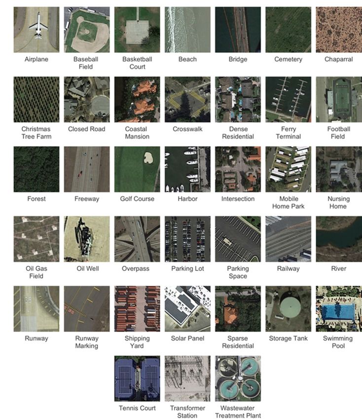
ISPRS Int. J. Geo-Inf. 2020, 9, 61                                                                      2 of 22

availability of the tags directly affect the performance of search engines. Therefore, this feature extraction
method has certain defects. On the other hand, some characteristics of the remote sensing images also
hinder the direct application of some commonly used image retrieval techniques (such as geometric
verification, query expansion, etc.). The remote sensing image contains not only one specific target but
also one or more targets and it also has rich geographic information, such as man-made buildings and
large-scale natural landscapes, such as trees, farmland, grassland and so forth. Specifically, the remote
sensing image covers a relatively large geographical area and can contain different numbers of different
semantic objects at the same time, which can be captured by the region at different scales. Although some
common remote sensing datasets contain many images that belong to the same semantic category, these
images are quite different. For instance, they may differ significantly in appearance or originate from
different geographic areas. In addition, the resolution level of remote sensing image and the height of
image acquisition will directly affect the size of the target object and some details. In summary, these
characteristics have led to certain difficulties and challenges in RSIR.
      With the further development of deep learning, CBIR has developed from the simple “artificial
descriptor” to the complex “convolutional descriptor” which can be extracted from the Convolutional
Neural Networks (CNNS) [6–8]. The deep convolutional neural network can establish the mapping
relationship between low-level features and high-level semantics. By extracting highly abstract image
information with high-level semantics, the accuracy of RSIR after deep neural network training is
better than RSIR based on traditional artificial features [9–11]. In addition, the deep features can be
automatically learned from the data without human effort, which makes deep learning techniques have
extremely important application value in large-scale RSIR research. Among them, Deep metric learning
(DML) is a technology that combines deep learning and metric learning [12]. The purpose of DML is to
learn the embedding space, which encourages the embedding vectors between similar samples to be
closer, while the dissimilar samples are far away from each other [13–15]. Deep metric learning uses the
discriminative ability of CNNS to embed images into metric space, where semantic metrics between
measured images can be directly calculated by simple metric algorithms such as Euclidean distance,
which makes the implementation process of the algorithm simpler. In addition deep metric learning
has been applied in many natural image domains, such as face recognition [12], visual tracking [16,17],
natural image retrieval [18], cross-model retrieval [19], geometric multi-manifold embedding [20] and
so forth. Although remote sensing images are quite different from ordinary natural images, deep
metric learning still has a full development prospect in CBRSIR.
      In the DML framework, the loss function plays a key role. With the development of research,
a number of loss functions have been proposed. Kaya M et al. [21] combined with recent research results,
revealed the importance of deep metric learning and summarized the current problems dealt with
in this filed. For instance, the contrastive loss [22,23] captures the similarity or dissimilarity between
pairwise of samples, while the triplet-based loss [12,24] describes the relationship among the triple
samples. Each triplet consists of an anchor sample, a positive sample and a negative sample. In general,
the triplet loss is better than contrastive loss due to the increased relationship between positive and
negative sample pairs. Inspired by this, recent researches have considered the richer representation of
structured information among multiple samples [25–28] and have achieved good performance in many
practical applications (such as image retrieval and image clustering). In particular, Wang et al. [29]
proposed a metric learning loss function based on the angular relationship of constrained triples in
negative samples, which is called “angular loss”. However, the most advanced DML methods still
have some limitations. First of all, we notice that when selecting samples for some loss functions,
only partial sample information is used and differences and permutations between sample classes
are ignored. In this case, not only are some non-trivial samples wasted but the relevant information
between the classes is not fully utilized. In Reference [30], researcher used all non-trivial samples with
non-zero loss (i.e., violating the pair constraint of query) to construct a structure with more information
to learn the embedding vectors, so as to avoid wasting the structural information of some non-trivial
samples. Although the information obtained by the method is abundant, some of them are redundant,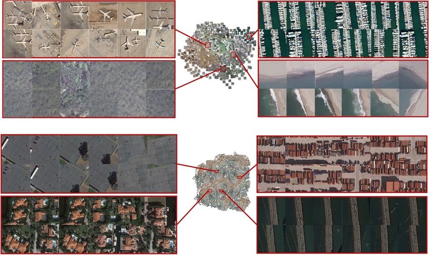
ISPRS Int. J. Geo-Inf. 2020, 9, 61                                                                   3 of 22

which would cause a considerable burden on the calculation cost and data storage. Secondly, the spatial
distribution of samples within the class is not considered in the above-mentioned losses but only the
similar samples are made as close as possible. Moreover, we observe that the previous losses are
equal to each positive sample, that is, they do not consider the impact of the quantitative relationship
between simple samples and hard samples on loss optimization. Ideally, a larger weight should be
given to a hard sample with a larger percentage. In Reference [31], the authors proposed Distribution
Structure Learning Loss (DSLL), which considers that the relative spatial structure of the initial state of
negative sample classes is maintained by weighting the negative sample classes. However, it does not
consider the influence of the relationship among the positive samples and the interaction between the
positive and negative samples on the spatial structure. The above methods would lose some similarity
structures and useful sample information within the class.
     Based on the above issues, this paper proposes a deep metric learning method based on the
Similarity Retention Loss (SRL). This method is improved in the following two aspects. The first is to
mine samples based on information pairs and the second is to assign different relative weights to all
selected samples. Firstly, we set different thresholds and selection strategies for positive and negative
samples to ensure that the selected samples are both representative and non-redundant. At the same
time, we recommend that attention should be paid to preserve the structural information within the
positive sample class during sample mining. Specifically, we just try to narrow the samples of the
same class to within a certain distance threshold, without forcing them to a point. Secondly, we assign
dynamic weights to selected hard samples according to the ratio of easy samples to hard samples
within the class and weight the loss of ranking consistency based on the distribution of negative sample
classes. We build an end-to-end fine-tuning network architecture for remote sensing image retrieval,
as shown in Figure 1. Our contributions in this paper are listed as follows:

1.     We propose the Similarity Retention Loss (SRL) for deep metric learning, which is completed by
       two iterative steps, samples mining and pair weights, as shown in Figure 1. The SRL considers
       the maintenance of similarity structures within and between classes, which makes the model
       more efficient and more accurate in collecting and measuring information pairs, thus improving
       the performance of image retrieval.
2.     We learn a threshold between similar samples to preserve the distribution of data within the class
       instead of narrowing down each class to a certain point in the embedding space. The efficient
       information retention within the class is considered so that the spatial structure features of each
       class are preserved in the feature space.
3.     By using an end-to-end fine-tuning network, we have performed extensive and comprehensive
       experiments on remote sensing datasets of PatternNet [11] and UCMD (UC Merced Land Use
       Dataset) [32] to validate the SRL theory. The results show that our method is significantly better
       than the state-of-the-art technology.

2. Related Work
     The fine-tuning network for remote sensing image retrieval consists of samples, network model
structure and loss function. These three compositions constitute a complete end-to-end image retrieval
system through deep metric learning training. In the following, we will discuss the related work on
our main contributions around these three aspects.

2.1. Fine-Tunning Network
     The fine-tuning of the network is an alternative method applied directly to a pre-trained network.
The method is initialized by a pre-trained classification network and then trained for different tasks.
Image feature learning on large-scale datasets (i.e., ImageNet) has strong generalization capabilities
and can be effectively migrated to other small-scale datasets [33]. In the process of CNN transfer
learning, the output value of the fully connected layer should be considered [7]. However, since the
ISPRS Int. J. Geo-Inf. 2020, 9, 61 4 of 22
value of the local feature of the convolutional layer expression image is relatively large [34], we usually
use convolutional layer features instead of fully connected layers.
ISPRS Int. J. Geo-Inf. 2019, 8, x FOR PEER REVIEW 4 of 23
Figure 1. The
Figure 1. The overall
overall framework
framework ofof our
our proposed
proposed Similarity
Similarity Retention
Retention LossLoss algorithm.
algorithm. The
The top
top is
is the
the
training
training process
process of
of the
the samples
samples in
in the
the network
network and
and the
the bottom
bottom is
is the
the testing
testing process.
process.
Pooling is another major concept in CNNS and is actually a form of down-sampling. Pooling layer
Pooling is another major concept in CNNS and is actually a form of down-sampling. Pooling
imitate the visual input system by reducing the dimension and abstraction of the visual input object.
layer imitate the visual input system by reducing the dimension and abstraction of the visual input
It has the following three functions—feature invariance, feature dimension reduction and avoidance
object. It has the following three functions—feature invariance, feature dimension reduction and
of over-fitting.
avoidance There are some
of over-fitting. Theregeneral
are some pooling
generalmodels,
poolingthe most common
models, of which of
the most common is which
sum pooling
is sum
proposed by Babenko and Lempitsky [35] and it performs well
pooling proposed by Babenko and Lempitsky [35] and it performs well in combination in combination with descriptor
with
whitening. Subsequently, Kalantidis et al. proposed weighted sum pooling
descriptor whitening. Subsequently, Kalantidis et al. proposed weighted sum pooling [36], which can[36], which can also be
seen as aseen
also be method of transfer
as a method learning.learning.
of transfer The hybrid Thescheme
hybridof linear of
scheme combination of maximum
linear combination and sum
of maximum
pooling is the R-Mac [37]. A global hybrid pooling is proposed for image
and sum pooling is the R-Mac [37]. A global hybrid pooling is proposed for image retrieval [38], retrieval [38], which is a
standard
which is alocal pooling
standard forpooling
local object recognition [39].
for object recognition [39].
In
In this paper, we first use the pre-trained network
this paper, we first use the pre-trained network to to fine-tune
fine-tune thethe network,
network, then
then select
select sample
sample
pairs from the remote sensing image dataset to train the network and finally
pairs from the remote sensing image dataset to train the network and finally optimize our proposed optimize our proposed
SRL for the
SRL for the final
finalremote
remotesensing
sensingimage
imageretrieval
retrieval task.
task. Observing
Observing thethe
remoteremote sensing
sensing data,
data, we find
we find that
that the image covers a large geographical area and the area contains rich
the image covers a large geographical area and the area contains rich background information andbackground information
and different
different numbers
numbers of different
of different semantic
semantic pairs.
pairs. We compared
We compared several
several common
common pooling
pooling methods
methods and
and choose
choose the the
most most appropriate
appropriate SPoC
SPoC (Sum-pooled
(Sum-pooled ConvolutionalFeatures)
Convolutional Features)pooling
poolinglayerlayer as
as the
the
aggregation
aggregation layer. This convergence
layer. This convergence layer
layer serves
serves as as the
the last
last layer
layer of
of fine-tuning
fine-tuning thethe convolutional
convolutional
neural
neural network
network to to build
build the
the system
system that
that is
is best
best suited
suited for
for CBRSIR.
CBRSIR.
2.2. Hard Sample Mining
2.2. Hard Sample Mining
Sample pair-based metric learning usually use a large number of paired samples but these samples
Sample pair-based metric learning usually use a large number of paired samples but these
often contain much redundant information. These redundant samples greatly reduce the actual
samples often contain much redundant information. These redundant samples greatly reduce the
function and convergence speed of the model. Therefore, the sampling strategy plays a particularly
actual function and convergence speed of the model. Therefore, the sampling strategy plays a
critical role in measuring the training speed of the learning model. In contrastive loss, the method of
particularly critical role in measuring the training speed of the learning model. In contrastive loss,
selecting training samples is the simplest, that is, randomly selecting positive and negative sample
the method of selecting training samples is the simplest, that is, randomly selecting positive and
pairs in the data. Initially, some researches on embedded learning tended to use the simple pairs
negative sample pairs in the data. Initially, some researches on embedded learning tended to use the
simple pairs training in Siamese network [23,40]. The Siamese network is composed of two
computing branches, each of which contains a CNN component. However, this method reduces the
convergence speed of the network.
In order to solve this problem, the hard negative mining methods have been proposed and
widely used [12,41–43]. Schroff et al. [12]. proposed a hard negative mining scheme by exploring
ISPRS Int. J. Geo-Inf. 2020, 9, 61                                                                   5 of 22

training in Siamese network [23,40]. The Siamese network is composed of two computing branches,
each of which contains a CNN component. However, this method reduces the convergence speed of
the network.
      In order to solve this problem, the hard negative mining methods have been proposed and widely
used [12,41–43]. Schroff et al. [12]. proposed a hard negative mining scheme by exploring semi-hard
triplets. The scheme defines a negative pair father than the positive. However, this negative mining
method only generate a small number of valid semi-hard triples and network training usually requires
large samples. Harwood et al. [41] proposed a framework called smart mining to collect the samples
from the entire dataset. The method will incur high off-line computing costs. Ge et al. [43] proposed
the Hierarchical Triplet Loss (HTL), which constructs a hierarchical tree of all categories and collects
hard negative pairs through dynamic margin. In Reference [42], the problem of sample mining in deep
metric learning was discussed and a distance weighted sample mining was proposed to select pairs of
negative samples.
      Although all samples within the threshold were mined by the above methods, the differences
between the negative sample classes and the influence of surrounding samples on the samples were
not considered. In this paper, the diversity and difference of samples are fully considered. Based on
this, we select multiple positive samples and negative samples of different classes and set the distance
to the samples according to the distribution of negative neighbor samples. We propose a new hard
samples mining method, that is, selecting different mining strategies to select positive sample pairs and
negative sample pairs by sorting the sample similarity and class information. In this way, the sample
selection is both representative and non-redundant, thereby achieving faster convergence and better
performance of the model.

2.3. Loss Functions for Deep Metric Learning
      The loss function plays a key role in deep metric learning. It is to increase or decrease the distance
between samples by adjusting the similarity between samples. In Reference [44], it is recommended
to use triplets as training samples to learn the feature space, where the similarity of the positive
sample pairs of triples is higher than that of the negative sample pairs. Specifically, the feature space
assigns equal weight to the selected sample pairs. In addition, quadruple loss functions have been
studied, such as histogram loss [45]. N-pair-mc [23] learns the embedded features by using the
structured relationship between multiple samples. The goal is to extract N-1 negative samples from
N-1 categories, one negative sample for each category and improve triplet loss by interacting with
more negative samples and categories. Concretely, the samples selected in N-pair loss are also assigned
the same weight. Movshovitz-Attias et al. proposed Proxy-NCA Loss [42], which uses a proxy instead
of the original sample to solve the sampling problem. Static proxy assignment is a proxy for each
class and its performance is better than dynamic proxy assignment. However, Proxy-NCA cannot
retain the scalability of DML, so the number of classes need to be proposed. Dong et al. proposed a
binomial deviance loss [46] and used binomial bias to evaluate the loss between labels and similarity.
Binomial deviance cost makes the model mainly train on the hard pairs, that is, the model focuses
more on negative samples near the boundary. Unlike the hinge loss, the binomial deviance loss assigns
different weights to the sample pairs based on their distance differences. Later, Song et al. proposed
Lifted Struct [25], which learns the embedded features by combining all negative samples. The purpose
of Lifted Struct is to draw the positive sample pair as close as possible and push all negative samples
to a position farther than the margin.
      Observing the above loss, triplet loss and N-pair loss give the same weight to the positive and
negative sample pairs. Unlike them, binomial Deviance Loss considers self-similarity and Lifted Struct
Loss sets weights for positive and negative sample pairs according to negative relative similarity.
However, these methods ignore the distribution of samples in the class and the differences between
different classes between classes. In this work, we propose the Similarity Retention Loss (SRL). We sort
all the samples except the query image according to the learned feature space similarity score with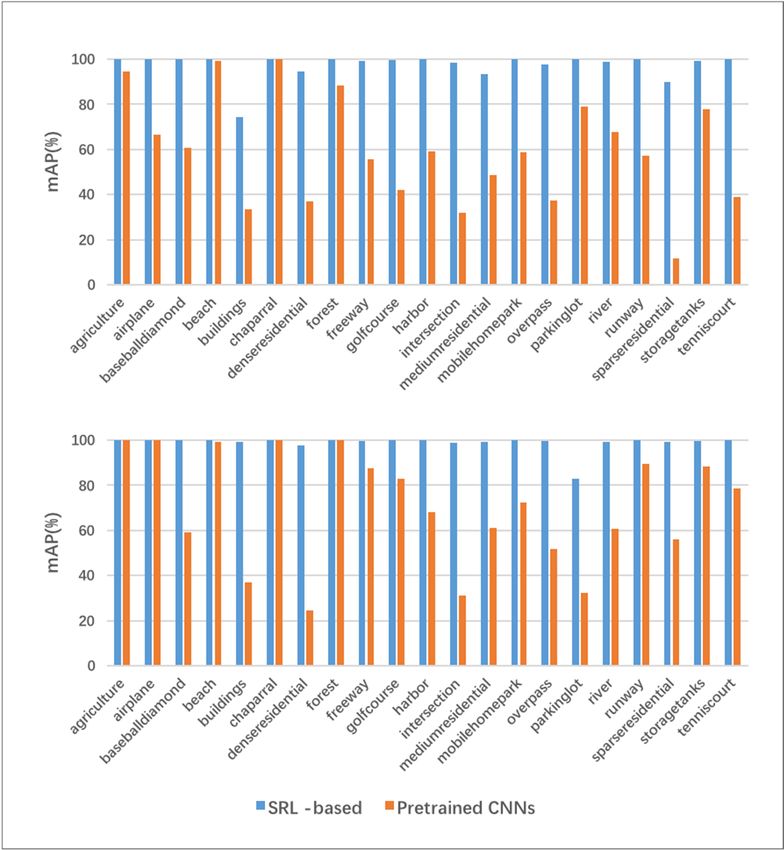
ISPRS Int. J. Geo-Inf. 2020, 9, 61                                                                                           6 of 22

the query. Then we weight the selected sample pairs according to the feature sorting and label, that
is, the degree to which each pair violates the constraint. SRL avoids the limitations of traditional
methods by merging a number of hard samples and exploring the inherently structured information.
For negative sample pairs, the distance should be as large as possible, so the higher the similarity,
 ISPRS Int. J. Geo-Inf. 2019, 8, x FOR PEER REVIEW                                              6 of 23
the  greater the impact and the higher the weight. For positive samples, on the contrary, the lower
the similarity, the more attention needs to be paid and the higher the weight. The illustration and
 illustration and comparison of different ranking-motivated losses and our method is presented in
comparison of different ranking-motivated losses and our method is presented in Figure 2.
 Figure 2.

         Figure 2. The
         Figure 2. The illustration
                       illustration and
                                    and comparison
                                        comparison of
                                                   of different
                                                      differentranking-motivated
                                                                ranking-motivatedlosses
                                                                                  lossesand
                                                                                         andour
                                                                                             ourmethod.
                                                                                                method.

3. The Proposed Approach
 3. The Proposed Approach
      Our target is to identify all examples that match this query image from other samples in the
       Our target is to identify all examples that match this query image from other                        n samplesoN in the
dataset,  given    any     query      image   of any class   in  the  remote  sensing   dataset.   Set X  =   x   , y        as the
 dataset, given anyquery            image of any class in the remote sensing dataset. Set X = (x , yi ) i=1 as the
                                                                                                                i
input
 input data,    where x(x
        data,where              , yi )represents
                             i, y       representsthe
                                                    thei-th  image
                                                          i-th image  whose
                                                                        whoseclass  label
                                                                                class     is y
                                                                                       label      y .The
                                                                                             isi .The number
                                                                                                         number  of classes    is C,
                                                                                                                      of classes   is
        yi ∈ y[1,∈2, 1,2,
                     . . . ,…
                            C],.CLet . LetXc X be the
                                        n oNc
 C, where
where                                              be theset set  of images
                                                              of images      in class
                                                                         in class      c,where
                                                                                   c, where  thethe   total
                                                                                                   total    number
                                                                                                         number          of images
                                                                                                                     of images    in
                                           i i=1
 in class c is
class c is N .  N  .
              c

3.1. Sampling
3.1. Sampling Mining
              Mining
        For the
       For   thequery
                 queryimages,
                          images,we wemine
                                         mineboth
                                               bothinformative
                                                        informativepositive
                                                                      positiveand  andnegative
                                                                                         negativesamples.
                                                                                                    samples. Given
                                                                                                                Given aa query
                                                                                                                          query
 sampleXX, ,we
sample      c    wesort
                     sortall
                           allother
                               othersamples
                                      samplesbyby     their
                                                    their    similarity
                                                           similarity    Xi .XP.i P
                                                                      to to c    c
                                                                                   is aiscollection
                                                                                           a collection   of same
                                                                                                     of the  the same
                                                                                                                   classclass as
                                                                                                                         as the
            i
 the query image which is expressed                 as   P  =   X  j ≠ i  , |P |  =  N   −  1.  N   is  a  collection of  other

query image which is expressed as Pci = Xcj j , i , Pci = Nc − 1. Nci is a collection of other images,
 images, denoted nas N = X k ≠ c, j ∈ 1,2,o … , N , P|N | = ∑ N . We create a dataset consisting of
                  c
denoted    as ,NP(X = Xk |k , c, j ∈ [1, 2, . . . , Nk ] , Nci =thek,c    Nk . We    create a dataset consisting of tuples
 tuples (X  i  ), j N(X )), where X represents                     query  image, P(X ) is the positive set that
   c      c         c
(X
 selected     , N XP
   i , P Xi from    i ),and  N(XX)ci is
                         where       represents
                                        the negative the query
                                                          set selected     P XciN is. The
                                                                  image,from          the positive
                                                                                            training set   thatpairs
                                                                                                       image    selected  from
                                                                                                                     consist  of
 these tuples, where each tuple corresponds to |P(X )| positive sample pairs and |N(X )| negative
 sample pairs.
        Positive sample set P(X ). Based on the spatial characteristics of the samples, we observe that
 the positive samples closer to the query not only do not have much useful information to train the
 network but also increase the cost of samples calculations. Therefore, based on the CNN descriptor
 distance, we select from P a fixed number of positive samples that are least similar to the query
 image as hard positive samples for training iterations. The choice of hard positive samples depends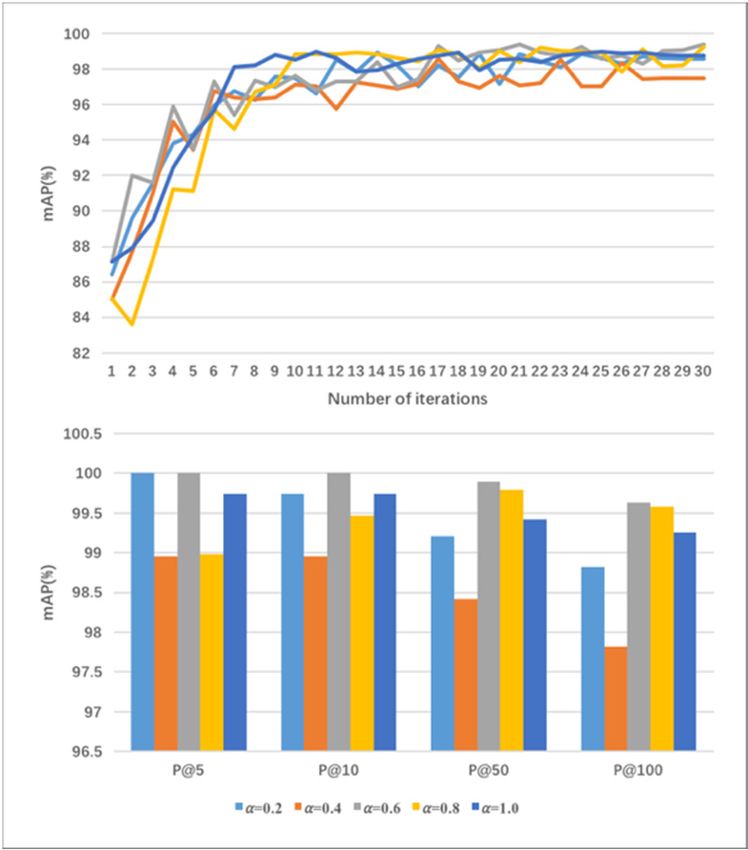
ISPRS Int. J. Geo-Inf. 2020, 9, 61 7 of 22
Pci and N Xci is the negative set selected from Nci . The training image pairs consist of these tuples,
where each tuple corresponds to P Xci positive sample pairs and N Xci negative sample pairs.
Positive sample set P Xci . Based on the spatial characteristics of the samples, we observe that the
positive samples closer to the query not only do not have much useful information to train the network
but also increase the cost of samples calculations. Therefore, based on the CNN descriptor distance,
we select from Pci a fixed number of positive samples that are least similar to the query image as hard
positive samples for training iterations. The choice of hard positive samples depends on the current
CNN’s parameters and is refreshed
per epoch.
Negative sample N Xci . Since the classes are non-overlapping, we select negative samples from
classes that are different from the class of the query image. We only select hard negative samples [47,48],
that is, mismatched samples with the most similar descriptor to the query image. K-nearest neighbors
from all mismatched samples are selected. At the same time, there are multiple similar samples in the
same class, which would lead to redundancy of sample information. A fixed number of samples each
class is allowed, which provide greater variability in the negative samples. The choice of hard negative
samples depends on the parameters of the current CNN and is refreshed multiple times per epoch.
3.2. Loss-Based Sample Weight
Our algorithm aims to bring the positive samples closer to the query image than any negative
samples, while pushing the negative samples farther than a predetermined boundary τ. In addition,
we try to separate the positive sample boundary from the negative sample boundary by the margin α,
that is, the positive samples are within the query sample τ − α distance. Therefore, α is the margin
between the negative and positive samples.
For each query image, the similarity between the selected positive and negative samples and
their similarity to the query sample are different. In order to make the most of them, we recommend
weighting them according to the loss value of the selected samples, that is, the degree to which each
sample pair violates the constraint.
We set a hard positive sample mining threshold between the positive samples and the query
according to the spatial distribution features of the samples. Assume that the distance between the
sample that is the least similar to the query sample and the query sample is margin. The positive
samples with a distance from the query image in the range of [0, threshold] are defined as easy positive
samples with high similarity to the query, while positive samples with a distance in the range of
[threshold, margin] are hard positive samples. The huge impact of hard positive samples in training will
weaken the influence of negative samples on gradient changes, which will not only affect the accuracy
of the network but also slow down the learning speed. Therefore, in this work, the number of hard
positive samples is used to limit the impact of positive samples on loss and to avoid an imbalance in the
loss of positive and negative samples during training. The threshold is set as τ − α, that is, the feature
distance threshold of the positive sample and the query image and we record the number of samples
in Pci with a distance greater than τ − α from the query as ni . Given the selected positive sample Xcj
(Xcj ∈ P Xci ), its weight wij+ can be calculated as:
2
Pci − ni
1
wij+
= ∗ 1 −
. (1)
P Xci Pci
For negative sample pairs, we propose a loss weight based on the negative sample order similarity
retention. The selection of negative samples is not continuous but is determined by two factors—sample
class and similarity with the query. From the perspective of class, the degree of difference between
the general characteristics of different negative sample classes and that of the class where the query
sample is located is different, so the learning level should also be different. At this time, the fixed
margin τ cannot work well. Suppose there are three classes, C, N1 , N2 , where C is the class of the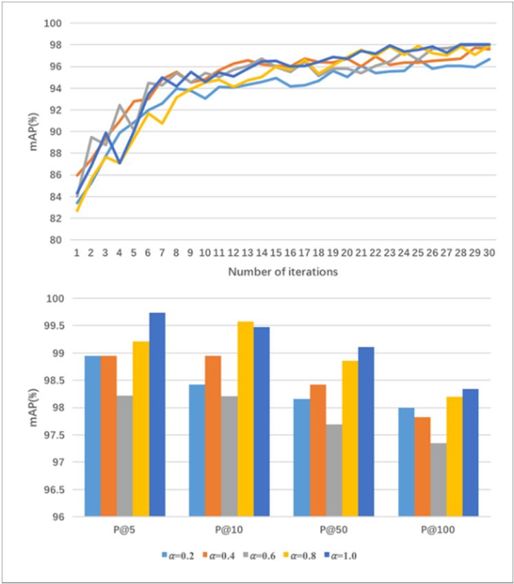
ISPRS Int. J. Geo-Inf. 2020, 9, 61 8 of 22
query image and N1 , N2 are different negative sample classes. If the difference between the N1 and C is
intuitively smaller than that between N2 and C, then the distance between N1 and C should be smaller
than that between N2 and C. However, when the margin value is fixed as set before, if the setting is
larger, the model may not be able to distinguish between N1 and C well. On the contrary, if the margin
is set smaller, N2 and C may not be distinguished well. At the same time, the similarity between the
negative samples and the query image is also different, so the impact on the training itself and the
required computational cost are also different. We assign different weights to each negative sample
class to maintain their relative similarity to the query sample, while ensuring that the
characteristics of
each class are retained. Specifically, given a selected negative sample Xkj (Xkj ∈ N Xci ), its weight w− ij
can be calculated as:
2
N Xci − rj
w−ij = 1 −
, (2)
N Xci
where rj is the sort position of the negative sample Xkj in the negative sample list N Xci .
3.3. Similarity Retention Loss
For each query Xci , we aim to make it father from the negative sample Nci than it is from the
positive samples Pci , with a minimum difference of α. Therefore, we pull samples from the same class
into the margin τ − α. We train the dataset on a two-branch network with the Siamese architecture.
Each branch is a clone of another branch, which means that they have the same hyper-parameters.
In order to bring together all positive samples in Pci , we minimize:
X 2
Lp Xci ; f = w+ c c
(
f Xi − f Xj − τ − α ) , j ∈ 1, 2, . . . , P Xci . (3)
Xc ∈P(Xc ) ij
j i +
Similarly, to push negative samples in Nci away from the boundary τ, we minimise:
X h i 2
LN Xci ; f = w−
ij ∗τ − f Xc
i − f Xk
j , j ∈ 1, 2, . . . , N Xci , (4)
Xkj ∈N(Xci ) +
where f is a discriminative function we learned, so that the similarity between the query and the positive
samples in the feature space is higher than the similarity between the query and the negative samples.
In SRL, we treat the two minimized objectives equally and optimize them jointly:
1
LSRL Xci ; f = (Lp Xci ; f + LN Xci ; f ). (5)
2
In order to reduce the amount of calculation and calculation time, we randomly select I (I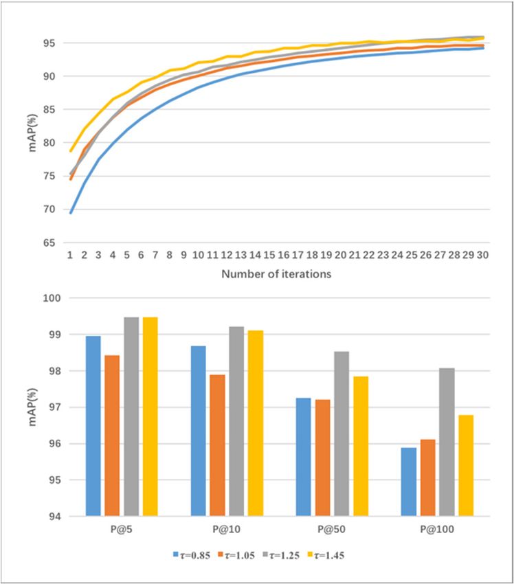
ISPRS Int. J. Geo-Inf. 2020, 9, 61 9 of 22
Algorithm 1 Similarity Retention Loss on Fine-tuning Network
Parameters Setting: The distance constraint τ on negative examples, the margin between positive and
1: negative examples α, the number of classes C, the number of images per class Nc (c ∈ C), the total number
of images N = C
P
i Ni , the number of query of per class I.
Input: the discriminative function f, the learning rate lr,
2: n oN n oN C n oI C
c
X = xi , yi = Xci ,the query list Q = Xcq
i=1 i=1 c=1 q=1 c=1
3: Output: Updated f.
4: Step 1: Forward all images into f to obtain the images’ embedding feature vector.
5: Step 2: Online iterative ranking and loss computation.
6: for each query Xcq do
7: Rank other images according to the similarity with the Xcq
8: Mine positive samples P Xcq .
9: Mine negative samples N Xcq .
10: Weigh positive samples using Equation (1).
11: Weigh negative samples
using Equation (2).
12: Compute Lp Xcq ; f using Equation (3).
13: Compute LN Xcq ; f using Equation (4).
14: Compute LSRL Xcq ; f using Equation (5).
15: end for
16: Compute LSRL (X; f) using Equation (6).
17: Step 3: Gradient computation and back propagation to update the parameters of f.
18: ∇ f = ∂LSRL (X; f)/∂ f
19: f = f − lr∗∇ f
4. Experiments
4.1. Datasets
This paper uses two published RSIR datasets, PatternNet [11] and UCMD [32], to evaluate our
proposed Similarity Retention Loss (SRL) for deep metric learning. The PatternNet [11] is a large-scale
remote sensing dataset with high-resolution collected for RSIR. It includes 38 classes, each of which has
800 images of 256 × 256 pixel size. This dataset is images of US cities collected through Google Map API
or Google Earth imagery. PatternNet contains images with different resolutions. The maximum spatial
resolution is about 0.062m and the minimum spatial resolution is about 4.693m. The representative
image of each class of the PatternNet dataset are shown in Figure 3, visually. The UCMD [32] is
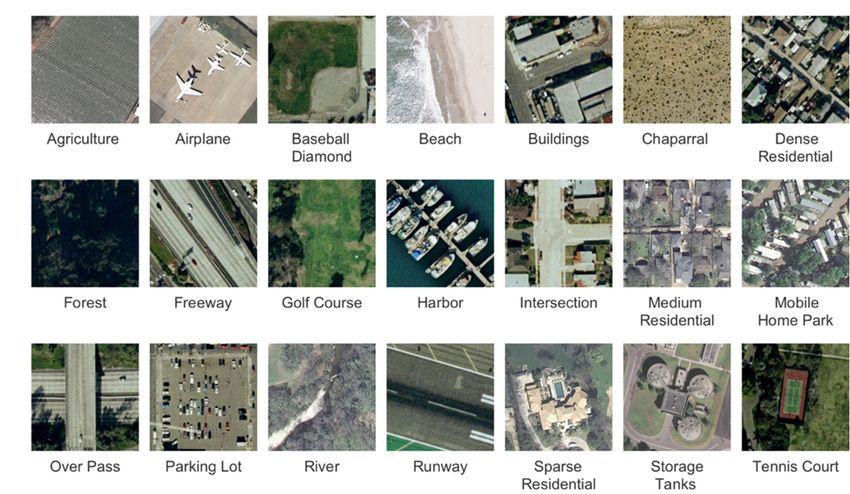
a land-cover or land-use dataset used as the RSIR benchmark dataset. It contains 21 classes with
100 images of 256 × 256 pixels per class. These images are segmented from large aerial images
downloaded by the USGS (United States Geological Survey), with a spatial resolution of approximately
0.3m. UCMD is a highly challenging dataset with some high overlapping categories such as the sparse,
medium and dense residential. A representative image of each class of the UCMD dataset are shown
in Figure 4, visually.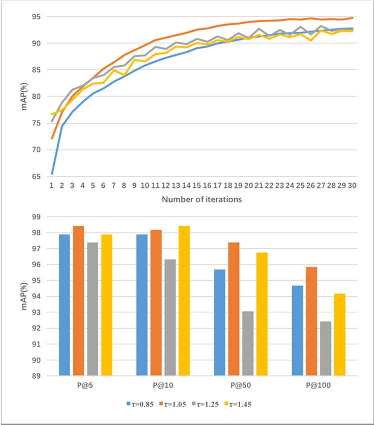
UCMD [32] is a land-cover or land-use dataset used as the RSIR benchmark dataset. It contains 21
classes with 100 images of 256 × 256 pixels per class. These images are segmented from large aerial
images downloaded by the USGS (United States Geological Survey), with a spatial resolution of
approximately 0.3m. UCMD is a highly challenging dataset with some high overlapping categories
 ISPRSas
such   Int.
         theJ. Geo-Inf.
               sparse,2020, 9, 61 and dense residential. A representative image of each class of the UCMD
                        medium                                                                        10 of 22

dataset are shown in Figure 4, visually.

      Figure 3. Illustration of the PatternNet. The PatternNet database covers 38 land-cover classes and one
     Figure
  ISPRS Int. J. 3. Illustration
                Geo-Inf. 2019, 8, xofFOR
                                      the PEER
                                          PatternNet.
                                               REVIEWThe PatternNet database covers 38 land-cover classes and10
                                                                                                              one
                                                                                                                of 23
      image of each class randomly selected from the PatternNet are shown.
     image of each class randomly selected from the PatternNet are shown.

      Figure      Illustrationofofthe
       Figure4.4. Illustration     theUCMD
                                       UCMD  (UC(UC  Merced
                                                   Merced      Land
                                                            Land UseUse  Dataset).
                                                                     Dataset).       The UCMD
                                                                               The UCMD           database
                                                                                            database covers covers
                                                                                                            21
      21 land-cover
       land-cover      classes
                    classes andand
                                oneone image
                                     image     of each
                                           of each classclass randomly
                                                          randomly      selected
                                                                   selected from from  the UCMD
                                                                                  the UCMD         are shown.
                                                                                             are shown.

4.2.
 4.2.Performance
      Performance Evaluation Metrics
                  Evaluation Metrics
      In
       Inthis
          this experiment,  we measure
                experiment, we  measurethethesimilarity
                                              similaritywith
                                                         withthe
                                                               theEuclidean
                                                                   Euclidean    distance
                                                                             distance andand
                                                                                           useuse
                                                                                               the the
                                                                                                    meanmean
Average   Precision  (mAP),  precision of the top-k (P@k)  and recall of the top-k  (R@k) to evaluate
 Average Precision (mAP), precision of the top-k (P@k) and recall of the top-k (R@k) to evaluate image image
retrieval
 retrievalperformance.
           performance.

4.3.
 4.3.Training
      TrainingSetup
               Setup.
      For
       For UCMD,
            UCMD, we adopt   adopt the
                                    the data
                                         datasegmentation
                                               segmentationstrategy
                                                              strategythat
                                                                        that  produces
                                                                           produces     thethe
                                                                                            bestbest performance
                                                                                                 performance    in in
Reference
 Reference[10],
             [10],that
                   thatis,is,randomly
                              randomlyselect
                                         select50%
                                                50%samples
                                                    samplesofofeach
                                                                eachcategory
                                                                     categoryfor fortraining
                                                                                     trainingand
                                                                                              andthe
                                                                                                   theremaining
                                                                                                       remaining50%
for
 50%testing. For PatternNet,
       for testing.              we usewe
                    For PatternNet,       80%/20%
                                             use 80%training and testing
                                                      / 20% training  anddata   segmentation
                                                                           testing              strategy from
                                                                                     data segmentation         [11].
                                                                                                         strategy
 from [11].
       Figure 5 presents the two CNNs used by our network (shown in Figure 1), which are used as the
 basic networks for feature extraction, namely VGG16 [49] and ResNet50 [50] . We use MatConvNet
 [51] to fine-tune the network. For the CNNs, only the convolutional layers are used to extract features.
 We remove the last pooling layer of the CNN networks and use the other convolutional layers as our
 basic CNN structure and then connect the SPoC pooling and L2 regularization to the new network
Average Precision (mAP), precision of the top-k (P@k) and recall of the top-k (R@k) to evaluate image
retrieval performance.
4.3. Training Setup.
ISPRS Int. J. For UCMD,
Geo-Inf. we
2020, 9, 61 adopt the data segmentation strategy that produces the best performance in
11 of 22
Reference [10], that is, randomly select 50% samples of each category for training and the remaining
50% for testing. For PatternNet, we use 80% / 20% training and testing data segmentation strategy
Figure 5 presents the two CNNs used by our network (shown in Figure 1), which are used as the
from [11].
Figurefor
basic networks 5 presents
feature the two CNNs
extraction, used by
namely our network
VGG16 (shown
[49] and in Figure
ResNet50 [50].1),We
which
useare used as the [51]
MatConvNet
basic networks for feature extraction, namely VGG16 [49] and ResNet50 [50] . We
to fine-tune the network. For the CNNs, only the convolutional layers are used to extract features.use MatConvNet
[51] to fine-tune
We remove the lastthe network.
pooling For the
layer of CNNs,
the CNN only networks
the convolutional
and uselayers
theare used convolutional
other to extract features.
layers
We remove the last pooling layer of the CNN networks and use the other convolutional layers as our
as our basic CNN structure and then connect the SPoC pooling and L2 regularization to the new
basic CNN structure and then connect the SPoC pooling and L2 regularization to the new network
network structure. In this experiment, the network is implemented based on the PyTorch framework.
structure. In this experiment, the network is implemented based on the PyTorch framework. Initialize
Initialize
the the parameters
parameters of each
of each network
network using
using the the corresponding
corresponding network
network weights
weights pre-trained
pre-trained on the
on the
ImageNet. We train the the
network with thethe
Adam −4
5 × 10momentum
ImageNet. We train network with Adamoptimizer,
optimizer, with
with weight decay5×10−4,
weight decay , momentum
0.9, proved by the
0.9, proved by increase of embedded
the increase of embedded dimension
dimensionandand the trainingtuple
the training tupleofof batch
batch size
size 5. 5.
(a) (b)
Figure
Figure 5. Convolutional
5. Convolutional Neural
Neural Network(CNN)
Network (CNN) network
network structure:
structure:(a)(a)
VGG16; (b) (b)
VGG16; ResNet50.
ResNet50.
ISPRS Int. J. Geo-Inf. 2019, 8, x FOR PEER REVIEW 11 of 23
4.4. Result and Analysis
4.4. Result and Analysis
4.4.1. Pooling Methods
4.4.1. Pooling Methods
In this section we compare the most advanced pooling methods—max pooling (MAC) [52], average
In this section we compare the most advanced pooling methods—max pooling (MAC) [52],
pooling (SPoC)
average [35] and
pooling Generalized
(SPoC) [35] and Mean poolingMean
Generalized (GeM) [33]. We
pooling use [33].
(GeM) the SRLWe loss
use for
the network
SRL losstraining
for
on the datasets
network with the
training learning
on the datasetsrate
with5e-8.
the Instead
learning of fine-tuning
rate theofpooling
5e-8. Instead layer
fine-tuning theofpooling
the lastlayer
layer of
the convolutional
of the last layerneural
of thenetwork, the above
convolutional neural three pooling
network, themethods
above threearepooling
used. Itmethods
can be concluded
are used. Itfrom
Figure 6 that
can SPoC is superior
be concluded to MAC
from Figure 6 thatand GeM
SPoC on all datasets.
is superior to MACInand general,
GeM on there are two main
all datasets. aspects to
In general,
thereofare
the error two main
feature aspects The
extraction. to the error
first of feature
is an increaseextraction. The first
in the variance of is
theanestimates
increase in theto
due variance of size
the finite
of thethe estimates due The
neighborhood. to the finite reason
second size of the neighborhood.
is that the error of The second reason is
the convolutional thatparameters
layer the error of leads
the to
convolutional
the offset layer parameters
of the estimated mean. The leads to thepooling
SPoC offset ofcan
theretain
estimated
moremean.
image Thebackground
SPoC pooling can retain by
information
more image background information by calculating the average value
calculating the average value of the image area, so as to reduce the occurrence of the first typeof the image area, so asoftoerror.
reduce the occurrence of the first type of error. This feature satisfies the large geographic area of the
This feature satisfies the large geographic area of the remote sensing images dataset, has rich background
remote sensing images dataset, has rich background information and contains different numbers of
information and contains different numbers of different semantic pairs, which makes the effect of SPoC
different semantic pairs, which makes the effect of SPoC better than other pooling methods in remote
bettersensing
than other
image pooling methods in remote sensing image retrieval.
retrieval.
(a) (b)
Figure 6. The pooling methods. Evaluation is performed with VGG16 (a) and ResNet50 (b) on
PatternNet
Figure datasets. The curve
6. The pooling represents
methods. the evolution
Evaluation of mAP
is performed withinVGG16
the training
(a) anditeration.
ResNet50 (b) on
PatternNet datasets. The curve represents the evolution of mAP in the training iteration.
4.4.2. Impact of the Negative Margin
As shown in the Section 3.2, for each query sample, SRL ensures the consistency of the structural
similarity order of the negative samples by adjusting the size of the negative sample space structure.
Since the constraint parameter τ determines the size of the negative space, we performed experimentsISPRS Int. J. Geo-Inf. 2020, 9, 61 12 of 22
4.4.2. Impact of the Negative Margin
As shown in the Section 3.2, for each query sample, SRL ensures the consistency of the structural
similarity order of the negative samples by adjusting the size of the negative sample space structure.
Since the constraint parameter τ determines the size of the negative space, we performed experiments
on the dataset to analyze the impact of the parameter τ.
In order to adapt the threshold τ to the PatternNet dataset and improve the performance of
different networks, the experiment selects a value of 0.5–1.5 and trains the network with a learning rate
of 0.00001. Finally, the results of τ = 0.85, 1.05, 1.25, 1.45 were selected according to the experiment,
as shown in Figure 7. The chart shown in Figure 7a is trained under VGG16, while Figure 7b represents
the dataset obtained under ResNet50 training. The results show that the optimal parameter τ for
VGG16 network is 1.05, while it is 1.25 for ResNet50. As can be seen from the graph, the performance
of the network increases with the increase of the threshold τ but when τ increases to a certain threshold,
the value decreases. This is because when the threshold value is small, the distance between the query
and negative samples is not enough to distinguish them. As the threshold τ increases, negative samples
with high similarity will decrease, which will affect the training effect. The results show that when
the thresholds are 1.05 (VGG6) and 1.25 (ResNet50), the difference between the positive and negative
samples is the best and the model results are the best. In the next experiment, we chose the threshold τ
= 1.05Int.
ISPRS forJ. the VGG16
Geo-Inf. 2019, 8,network andREVIEW
x FOR PEER 1.25 for the ResNet50. 12 of 23
(a) (b)
Figure 7. The impact of the different threshold τ. Evaluation is performed with VGG16 (a) and
ResNet50 (b) on PatternNet datasets. The curve represents the evolution of mAP in the training
Figure 7. The impact of the different threshold τ. Evaluation is performed with VGG16 (a) and
iteration. The histogram shows the evaluation of P@K under different thresholds τ.
ResNet50 (b) on PatternNet datasets. The curve represents the evolution of mAP in the training
4.4.3.iteration.
Impact of the
The Parameter
histogram shows
α the evaluation of P@K under different thresholds τ.
The threshold τ is used to control the distance that the negative samples are pushed away, while
4.4.3. Impact of the Parameter α
the threshold α is used to control the degree of aggregation of the positive samples, that is, the distance
The threshold
between the positiveτ isand
used to control
negative the distance
samples. that thethe
By setting negative samples
threshold α, theare pushedbetween
distance away, while
the
the threshold
positive α is used
and negative to control
samples can be the degree
pulled whileofmaintaining
aggregation theofspatial
the positive
structuresamples, thatpositive
among the is, the
distance between
samples. the positive
As described andinnegative
in 4.4.2, VGG16,samples. By setting
we performed the threshold
an experiment of α, the distance
threshold between
α under the
the positive
condition and
of τ negative
= 1.05 and insamples
ResNet50,canwe
be set
pulled while maintaining the spatial structure among the
τ = 1.25.
positive samples. As described in 4.4.2, in VGG16, we performed an experiment of threshold α under
the condition of τ=1.05 and in ResNet50, we set τ=1.25.
In the experiment, the values of the threshold α are 0.2, 0.4, 0.6, 0.8 and 1.0, respectively. The
experimental results are shown in Figure 8. The results show that when we set α =1.0, the best result
is obtained in VGG16 (a). And in ResNet50 (b), the best result is obtained at α =0.6. That’s because
when the α is small, the distance between the positive and negative samples is not large enough, soISPRS Int. J. Geo-Inf. 2020, 9, 61 13 of 22
In the experiment, the values of the threshold α are 0.2, 0.4, 0.6, 0.8 and 1.0, respectively.
The experimental results are shown in Figure 8. The results show that when we set α = 1.0, the best
result is obtained in VGG16 (a). And in ResNet50 (b), the best result is obtained at α = 0.6. That’s
because when the α is small, the distance between the positive and negative samples is not large
enough, so that the network after training cannot clearly distinguish them. Conversely, when α is too
large, the spatial structure inside the positive sample cannot be maintained. Therefore, the network
can achieve the best effect only when the value of α can distinguish the positive and negative samples
and
ISPRSmaintain the2019,
Int. J. Geo-Inf. positive sample
8, x FOR space structure.
PEER REVIEW 13 of 23
(a) (b)
Figure 8. The impact of the different threshold α. Evaluation is performed with VGG16 (a) and
ResNet50 (b) on PatternNet datasets. The curve represents the evolution of mAP in the training
Figure 8. TheThe
iteration. impact of the shows
histogram different evaluationα.ofEvaluation
thethreshold P@K underisdifferent
performed with VGG16
thresholds α. (a) and ResNet50
(b) on PatternNet datasets. The curve represents the evolution of mAP in the training iteration. The
4.4.4. Ceteris Paribus Analysis
histogram shows the evaluation of P@K under different thresholds α.
In this section, we study in more benefits of using the method Similarity Retention Loss over
other structural
4.4.4. Ceteris losses.
Paribus For this purpose, we replace the proposed SRL in our approach with the
Analysis
Triplet Loss [44], N-pair-mc Loss [23], Proxy-NCA Loss [42], Lifted Struct Loss [25] and Distribution
In this section, we study in more benefits of using the method Similarity Retention Loss over
Structure Learning Loss (DSLL) [31]. We then re-train the network, keeping the network structure
other structural losses. For this purpose, we replace the proposed SRL in our approach with the
(ResNet50) identical and separately re-tuning some hyper-parameters, such as the weight decay and
Triplet Loss [44], N-pair-mc Loss [23], Proxy-NCA Loss [42], Lifted Struct Loss [25] and Distribution
the learning rate. In the experiment, we use the mean Average Precision (mAP), precision of the top-k
Structure Learning Loss (DSLL) [31]. We then re-train the network, keeping the network structure
(P@k) and recall of the top-k (R@k) to evaluate image retrieval performance. The UCMD dataset
(ResNet50) identical and separately re-tuning some hyper-parameters, such as the weight decay and
used in the experiment contains 21 classes of 100 images per class. We randomly select 50% of each
the learning rate. In the experiment, we use the mean Average Precision (mAP), precision of the top-
class for training and the remaining 50% for testing (i.e., 50 images of each class). According to
k (P@k) and recall of the top-k (R@k) to evaluate image retrieval performance. The UCMD dataset
the quantitative characteristic of UCMD dataset, we choose Recall at top 25, 40, 50, 100 as one of
used in the experiment contains 21 classes of 100 images per class. We randomly select 50% of each
the evaluation criteria for the test result. We randomly select 80% of each class of images from the
class for training and the remaining 50% for testing (i.e., 50 images of each class). According to the
PatternNet dataset (containing 38 classes, 800 images per class) as the training set and the remaining
quantitative characteristic of UCMD dataset, we choose Recall at top 25, 40, 50, 100 as one of the
20% as the test set (i.e., 160 images of each class are used as the test set). So we select Recall at top 80,
evaluation criteria for the test result. We randomly select 80% of each class of images from the
100, 160, 200 as the evaluation criteria for the test result of the PatternNet dataset. We evaluate the
PatternNet dataset (containing 38 classes, 800 images per class) as the training set and the remaining
proposed algorithm on image retrieval tasks in comparison with the advanced metric learning loss
20% as the test set (i.e., 160 images of each class are used as the test set). So we select Recall at top 80,
algorithms. Performance after training is presented in the Tables 1 and 2. As can be seen from the
100, 160, 200 as the evaluation criteria for the test result of the PatternNet dataset. We evaluate the
table, the accuracy of our method is higher than others. When using the ResNet50 network framework,
proposed algorithm on image retrieval tasks in comparison with the advanced metric learning loss
compared with the DSLL, SRL provides a significant improvement of +1.26% in mAP and +1.12% in
algorithms. Performance after training is presented in the Table 1 and Table 2. As can be seen from
the table, the accuracy of our method is higher than others. When using the ResNet50 network
framework, compared with the DSLL, SRL provides a significant improvement of +1.26% in mAP
and +1.12% in R@50 on UCMD dataset. Furthermore, the SRL signatures achieves a gain of +1.07% in
mAP and +0.98% in R@160 on PATTERNNET dataset, which surpassed recently published DSLL and
achieves mAP of 99.41%, P@10 of 100 and R@180 of 99.96%. In general, our approach is demonstratedISPRS Int. J. Geo-Inf. 2020, 9, 61 14 of 22
R@50 on UCMD dataset. Furthermore, the SRL signatures achieves a gain of +1.07% in mAP and
+0.98% in R@160 on PATTERNNET dataset, which surpassed recently published DSLL and achieves
mAP of 99.41%, P@10 of 100 and R@180 of 99.96%. In general, our approach is demonstrated to be the
most effective. This is because we use a new method of mining samples through spatial distribution
and the loss of similarity retention calculation for all selected samples.
Table 1. The evaluation results of mAP and P@K on the PatternNet and UCMD database comparing
with the other structure loss.
Dataset Structural Loss mAP P@5 P@10 P@50 P@100 P@1000
Triplet Loss 92.94 98.52 96.92 92.13 46.07 4.61
N-pair-mc Loss 91.11 94.94 91.15 90.33 45.17 4.52
Proxy-NCA Loss 95.71 97.56 96.69 94.89 47.45 4.74
UCMD
Lifted Struct Loss 96.58 98.05 97.62 95.75 47.88 4.79
DSLL 97.52 98.09 98.03 96.68 48.34 4.83
SRL 98.78 99.63 99.56 99.33 48.96 4.90
Triplet Loss 94.96 99.04 97.63 96.62 95.16 15.69
N-pair-mc Loss 94.81 97.04 95.46 94.49 95.08 15.67
Proxy-NCA Loss 97.72 98.98 98.65 98.23 98.02 15.71
PatternNet
Lifted Struct Loss 98.09 98.90 98.82 98.78 98.46 15.76
DSLL 98.34 99.05 98.98 98.93 98.67 15.86
SRL 99.41 100 100 99.55 99.24 15.90
Table 2. The evaluation results of R@K on the PatternNet and UCMD database comparing with the
other structure loss methods.
Dataset Structural Loss R@25 R@40 R@50 R@100
Triplet Loss 47.75 76.99 91.23 96.21
N-pair-mc Loss 45.39 75.57 90.19 95.65
Proxy-NCA Loss 48.56 77.47 96.92 99.14
UCMD
Lifted Struct Loss 49.04 77.11 97.13 99.26
DSLL 49.63 78.06 97.31 99.28
Similarity Retention Loss 49.71 78.48 98.43 99.95
Dataset Structural Loss R@100 R@130 R@160 R@180
Triplet Loss 48.85 77.52 96.32 98.61
N-pair-mc Loss 48.80 77.38 95.97 98.36
Proxy-NCA Loss 48.97 78.60 97.31 99.17
PatternNet
Lifted Struct Loss 49.01 78.64 97.51 99.28
DSLL 49.16 79.03 98.30 99.33
Similarity Retention Loss 49.96 79.78 99.28 99.96
4.4.5. Overall Results and Per-Class Results
We present experiments on the PatternNet and UCMD datasets, with margin τ = 1.05 for
VGG16 and 1.25 for ResNet50. In this experiments we set margin α = 1.0 for VGG16 and 0.6 for
ResNet50. The final results of the PatternNet and UCMD datasets are shown in Table 3. It can be
seen that, compared to the state-of-the-art performance, the SRL-based features can achieve optimal
performance. When using the VGG16 network framework, compared with the MiLaN, SRL provides a
significant improvement of +7.38% in mAP on UCMD dataset. Furthermore, the SRL achieves a gain of
+24.92% in mAP and +3.67% in P@10 on PATTERNNET dataset, which surpassed recently published
GCN (Graph Convolutional Networks). When using the ResNet50 network framework, on the UCMD
dataset, the experimental results achieve +8.38% growth compared to MiLaN in mAP and achieve
mAP of 99.41%, P@10 of 100 and offer over 73.11%, 95.53% gain over the GCN on PATTERNNET
dataset. At the same time, we find that although the effect of the EDML (Enhancing Remote Sensing
Image Retrieval with Triplet Deep Metric Learning Network) [53] on the PatternNet dataset is slightlyISPRS Int. J. Geo-Inf. 2020, 9, 61 15 of 22
higher than our SRL, for example, the EDML achieves a gain of +1.40% and +0.14% in mAP on
PatternNet database, which trained respectively on the VGG16 network and ResNet50. But based on
comprehensive experimental results, our SRL is the best. First, from the results (Table 3), our method
can effectively improve the accuracy of the network on the UCMD dataset (the number of images in
the dataset is smaller). Specific example—the SRL method gains +2.91% and +2.15% on the mAP
obtained after training on the VGG16 network and the ResNet50 network, respectively, which exceeds
the result of EDML. This shows that our method is more friendly to the dataset with insufficient images,
which is very meaningful in image retrieval. Second, we find that the sample mining strategy adopted
by the EDML is to randomly pick positive samples from the same class as the anchor (except the
anchor) and negative samples from any other classes. This strategy has some disadvantages. (1) The
representativeness of the samples is difficult to guarantee; (2) The work of obtaining samples is heavy;
(3) It makes the training convergence time longer. In order to verify the advantages of the proposed
SRL algorithm model in terms of training speed, we reproduce the EDML and compare the training
time of the model with our model. We conduct experiments on Intel® i7-8700, 11 GB memory CPU,
Ubuntu 18.04LTS operating system and use VGG16 and ResNet50 as the basic network to calculate
the training time. The results show that the training time of 70 epochs of UCMD database using
EDML algorithm in VGG16 and ResNet50 network is 9.8 h and 27.8 h respectively, while the training
time of PatternNet dataset is 11.6 h and 30.9 h respectively. Training with SRL took 8.2 h (VGG16,
UCMD), 24.4 h (ResNet50, UCMD), 9.9 h (VGG16, PatternNet) and 27.6 h (ResNet50, PatternNet).
In general, our approach is demonstrated to be the most effective. To summarize, on both remote
sensing datasets like UCMD dataset and PatternNet dataset, our method achieves new state-of-the-art
or comparable performance.
Interestingly, the best performance on PatternNet is significantly better than the UCMD.
One possible reason is that data-driven is a major feature of deep metric learning and the learning
performance of representative features is affected by the amount of training data. PatternNet has
a larger amount of data than UCMD, so the network for the former is better trained than the latter.
The image retrieval visualized results of PatternNet and UCMD trained under the ResNet50 network
are shown in Figure 9.
Table 3. Evaluation results on the PatternNet and UCMD database comparing with the
state-of-the-art methods.
Dataset Feature mAP P@5 P@10 P@50 P@100 P@1000
Gabor Texture [11] 27.73 68.55 62.78 44.61 35.52 8.99
VLAD [11] 34.10 58.25 55.70 47.57 41.11 11.04
UFL [11] 25.35 52.09 48.82 38.11 31.92 9.79
VGGF Fc1 [11] 61.95 92.46 90.37 79.26 69.05 14.25
VGGF Fc2 [11] 63.37 91.52 89.64 79.99 70.47 14.52
VGGS Fc1 [11] 63.28 92.74 90.70 80.03 70.13 14.36
VGGS Fc2 [11] 63.74 91.92 90.09 80.31 70.73 14.55
ResNet50 [11] 68.23 94.13 92.41 83.71 74.93 14.64
LDCNN [11] 69.17 66.81 66.11 67.47 68.80 14.08
PatternNet G-KNN [54] 12.35 - 13.24 - - -
RAN-KNN [54] 22.56 - 37.70 - - -
VGG-VD16 [54] 59.86 - 92.04 - - -
VGG-VD19 [54] 57.89 - 91.13 - - -
GoogLeNet [54] 63.11 - 93.31 - - -
GCN [54] 73.11 - 95.53 - - -
SGCN [54] 71.79 - 97.14 - - -
EDML (VGG16) [53] 99.43 99.53 99.50 99.47 99.46 15.90
EDML (ResNet50) [53] 99.55 99.58 99.57 99.57 99.54 15.90
SRL (VGG16) 98.03 99.86 99.20 98.41 98.26 15.90
SRL (ResNet50) 99.41 100 100 99.55 99.24 15.90You can also read