Manifold Regularized Dynamic Network Pruning
←
→
Page content transcription
If your browser does not render page correctly, please read the page content below
Manifold Regularized Dynamic Network Pruning

                                             Yehui Tang1,2 , Yunhe Wang2 *, Yixing Xu2 , Yiping Deng3 , Chao Xu1 , Dacheng Tao4 , Chang Xu4
                                                             1
                                                              Key Lab of Machine Perception (MOE), Dept. of Machine Intelligence, Peking University.
                                                        2
                                                             Noah’s Ark Lab, Huawei Technologies. 3 Central Software Institution, Huawei Technologies.
                                                                   4
                                                                     School of Computer Science, Faculty of Engineering, University of Sydney.
                                                                   yhtang@pku.edu.cn; yunhe.wang@huawei.com; c.xu@sydney.edu.au
arXiv:2103.05861v1 [cs.CV] 10 Mar 2021

                                                                       Abstract                              bile phones and wearable devices, techniques that effec-
                                                                                                             tively reduce the cost of modern deep networks are re-
                                             Neural network pruning is an essential approach for             quired [31, 13, 58, 60].
                                         reducing the computational complexity of deep models so                 To this end, a number of model compression algo-
                                         that they can be well deployed on resource-limited devices.         rithms have been developed without affecting network per-
                                         Compared with conventional methods, the recently devel-             formance. For instance, quantization [53, 14, 43, 57] uses
                                         oped dynamic pruning methods determine redundant filters            less bits to represent network weights and knowledge dis-
                                         variant to each input instance which achieves higher accel-         tillation [19, 54, 4, 40, 55] is to train a compact network
                                         eration. Most of the existing methods discover effective sub-       based on the knowledge of a teacher network. Low-rank ap-
                                         networks for each instance independently and do not utilize         proximation [35, 24, 29] tries to decompose the original fil-
                                         the relationship between different inputs. To maximally ex-         ters to smaller ones while pruning method directly discards
                                         cavate redundancy in the given network architecture, this           the redundant neurons to get a sparser network. Among
                                         paper proposes a new paradigm that dynamically removes              them, channel pruning (or filter pruning) [18, 49, 36, 33]
                                         redundant filters by embedding the manifold information of          is regarded as a kind of structured pruning method, which
                                         all instances into the space of pruned networks (dubbed as          directly discards redundant filters to obtain a compact net-
                                         ManiDP). We first investigate the recognition complexity            work with lower computational cost. Since the pruned net-
                                         and feature similarity between images in the training set.          work can be well employed on mainstream hardwares to ob-
                                         Then, the manifold relationship between instances and the           tain considerable speed-up, channel pruning is widely used
                                         pruned sub-networks will be aligned in the training proce-          in industrial products.
                                         dure. The effectiveness of the proposed method is verified              The conventional channel pruning methods obtain a
                                         on several benchmarks, which shows better performance in            static network applied to all input samples, which do not
                                         terms of both accuracy and computational cost compared to           excavate redundancy maximally, as the diverse demands for
                                         the state-of-the-art methods. For example, our method can           network parameters and capacity from different instances
                                         reduce 55.3% FLOPs of ResNet-34 with only 0.57% top-1               are neglected. In fact, the importance of filters is highly
                                         accuracy degradation on ImageNet.                                   input-dependent. A few methods proposed recently prune
                                                                                                             channels according to individual instances dynamically and
                                                                                                             achieve better performance. For example, Gao et al. [9] in-
                                         1. Introduction                                                     troduce small auxiliary modules to predict the saliencies of
                                                                                                             channels with given input data, and prune unimportant fil-
                                            Deep convolutional neural networks (CNNs) have
                                                                                                             ters at run-time. Instance-wise sparsity is adopted in [32] to
                                         achieved state-of-the-art performance on a large variety of
                                                                                                             induce different sub-networks for different samples. How-
                                         computer vision tasks, e.g., image classification [15, 48,
                                                                                                             ever, the existing methods prune channels for individual in-
                                         23, 59], objection detection [10, 44, 11], and video anal-
                                                                                                             stances independently, which neglects the relationship be-
                                         ysis [7, 12, 21]. Besides the model performance, recent
                                                                                                             tween different instances. A sparsity constraint with same
                                         researches pay more attention on the model efficiency, es-
                                                                                                             intensity is usually used for different input instances, re-
                                         pecially the computational complexity [56, 47, 46]. Since
                                                                                                             gardless of the diversity of instance complexity. Besides,
                                         there are considerable real-world applications required to
                                                                                                             the similarity between instances is also valuable informa-
                                         be deployed on resource constrained hardwares, e.g., mo-
                                                                                                             tion deserving to explore.
                                           * Corresponding   author.                                             In this paper, we explore a new paradigm for dynamic

                                                                                                         1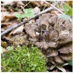
…
                        …                                                                                   …
                                                   Similarity

                   Input Images            Manifold Regularization       Original Network          Pruned Sub-Networks
Figure 1. Diagram of the proposed manifold regularized dynamic pruning method (ManiDP). We first investigate the complexity and
similarity of images in the training dataset to excavate the manifold information. Then, the network is pruned dynamically by exploiting
the manifold regularization.
pruning to maximally excavate network redundancy corre-                  mance on several benchmarks. For example, Molchanov et
sponding to arbitrary instance. The manifold information                 al. [37] uses Taylor expansion to estimate the contribution
of all samples in the given dataset is exploited in the train-           of a filter to the final output and discard filters with small
ing process and corresponding sub-networks are derived to                scores, while Liebenwein et al. [27] construct an impor-
preserve the relationship between different instances (Fig-              tance distribution that reflects the filter importance. To re-
ure 1). Specifically, we first propose to identify the com-              duce the disturbance of irrelevant factors, Tang et al. [49]
plexity of each instances in the training set and adaptively             set up a scientific control during pruning filters, which can
adjust the penalty weight on channel sparsity. Then, we fur-             discover compact networks with high performance. These
ther preserve the similarity between samples in the pruned               methods prune same filters for different input instances and
results, i.e., the sub-network for each input sample. In prac-           obtain a ’static’ network with limited representation capa-
tice, the features with abundant semantic information ob-                bility, whose performance degrades obviously when a large
tained by the network are used for calculating the simi-                 pruning rate is required.
larity. By exploiting the proposed approach, we can allo-                    Dynamic Pruning. Beyond the static pruning methods,
cate the overall resources more reasonably, and then ob-                 an alternative way is to determine the importance of filters
tain pruned networks with higher performance and lower                   according to input data, and skip unnecessary calculation
costs. Experiments are throughly conducted on a series of                in the test phase [42]. Dong et al. [6] use low-cost col-
benchmarks for demonstrating the effectiveness of the new                laborative layers to induce sparsity on the original convo-
method. Compared with the state-of-the-art pruning algo-                 lutional kernels at the running time. Hua et al. [20] gener-
rithms, we obtain higher performance in terms of both net-               ate decision maps by partial input channels to identify the
work accuracy and speed-up ratios.                                       unimportant regions in feature maps. However, the skipped
    The rest of this paper is organized as follows: Section 2            ineffective regions in [20] are irregular and practical accel-
briefly reviews the existing channel pruning methods and                 eration depends on special hardware such as FPGAs and
Section 3 introduces the formulations. We discuss the pro-               ASICs. Gao et al. [9] introduces squeeze-excitation mod-
posed method in Section 4 and conduct extensive experi-                  ules to predict the saliency of channels and skip those with
ments in Section 5. Finally, Section 6 summarizes the con-               less contribution to the classification results. Complemen-
clusions.                                                                tary to them, this paper focuses on effectively training the
                                                                         dynamic network to allocate a proper sub-network for each
2. Related Work                                                          instance, which is vital to achieve a satisfactory trade-off
                                                                         between accuracy and computational cost.
   Channel Pruning is a kind of coarse-grain structural
pruning method that discards the whole redundant filters to              3. Preliminaries
obtain a compact network, which can achieve practical ac-
celeration without specific hardware [52, 50, 30, 33, 3]. It                 In this section, we introduce the formulations of channel
contains the conventional static pruning methods and recent              pruning for deep neural networks and the dynamic pruning
dynamic algorithms, and we briefly review them as follows.               problem.
   Static Pruning. A compact network shared by different                     Denote the dataset with N samples as X = {xi }N        i=1 ,
instances is desired in static pruning. Wen et al. [52] impose           and Y = {yi }N     i=1 are the corresponding labels. For a
                                                                                                                 l  l−1    l   l
structural sparsity on the weights of convolutional filters to           CNN model with L layers, W l ∈ Rc ×c ×k ×k denotes
discover and prune redundant channels. Liu et al. [33] as-               weight parameters of the convolution filters in the l-th layer.
                                                                                         l   l  l
sociates a scaling factor to each channel and the sparsity               F l (xi ) ∈ Rc ×w ×h is the output feature map of the l-th
                                                                                       l
regularization is imposed on the factors. Recently, more                 layer with c channels, which can be calculated with con-
methods are proposed which achieve state-of-the-art perfor-              volution filters W l and the features F l−1 (xi ) in the previ-

                                                                     2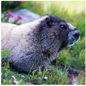
ous layer, i.e., F l (xi ) = ReLU (F l−1 (xi ) ∗ W l ), where                    Lce (xi , W) and the sparsity regularization, i.e.,
∗ denotes the convolutional operation and ReLU (t) =
                                                                                                N                          L
max(t, 0) is the activation function.                                                           X                          X
                                                                                          min         Lce (xi , W) + λ ·         kπ l (xi )k1 ,   (3)
    Channel pruning discovers and eliminates redundant                                     W
                                                                                                i=1                        l=1
channels in a given neural network to reduce the over-
all computational complexity while retaining a comparable                        where kπ l (xi )k1 is the `1 -norm penalty on the channel
performance [52, 33, 37, 27]. Basically, the conventional                        saliency π l (xi ). Obviously, a larger coefficient λ also pro-
channel pruning can be formulated as                                             duces sparer saliency π l (xi ) and thus yields more com-
                  N                           L
                                                                                 pact networks with lower computational cost. Compared
                  X                           X                                  to the static pruning method (Eq. (1)) that uses a same
            min         Lce (xi , W) + λ ·          kW l k2,1         (1)
             W                                                                   compact network to handle all the input data, the dynamic
                  i=1                         l=1
                                                                                 one (Eq. (3)) aims to prune channels for different instances
where W denotes all the weight parameters of the network,                        accordingly.
and Lce (xi , W) is the task-dependent loss function (e.g.,
the cross-entropy loss for classification task). k · k2,1 is the                 4. Manifold Regularized Dynamic Pruning
`21 -norm that induces channel-wise sparsity on convolution
                                Pcl                                                  The main purpose of dynamic pruning is to fully ex-
filters, i.e., kW l k2,1 =                          l
                                  j=1 kvector(Wj,:,:,: )k2 , where
                                         l
                                                                                 cavate the network redundancy for each instance. How-
vector(·) straightens the tensor Wj,:,:,:       to vector form and               ever, the manifold information, i.e., the relationship be-
                          1
k · k2 is the `2 -norm . The trade-off coefficient λ balances                    tween samples in the entire dataset has rarely been studied.
the two losses, and a larger λ induces sparser convolution                       The manifold hypothesis states that the high-dimensional
kernel W l and then obtain a more compact network.                               data can be embedded into low-dimensional manifold, and
     Dynamic pruning is developed for further excavating                         samples locate closely in the manifold space own analo-
the correction between input instances and pruned chan-                          gous properties. The mapping function from input samples
nels [9, 42, 20]. Wherein, the importance of output channels                     to their corresponding sub-networks should be smooth over
depends on the inputs, and different sub-networks will be                        the manifold space, and then the relationship between sam-
generated for each individual instance for flexibly discover-                    ples need to be preserved in sub-networks. This manifold
ing the network redundancy. To this end, a control module                        information can effectively regularize the solution space
G l is introduced to process the input feature F l−1 (xi ) and                   of instance-network pairs to help allocate a proper sub-
predict the channel saliency π l (xi , W) = G l (F l−1 (xi )) ∈                  network for each instance. In the following, we explore the
    l
Rc in the l-th layer for input xi .2 In practice, a smaller                      manifold information from two complementary perspec-
element in π l (xi ) implies that the corresponding channel                      tives, i.e., complexity and similarity.
is less important. The controller G is usually implemented
by utilizing a squeeze-excitation module as suggested in [9].                    4.1. Instance Complexity
Then, redundant channels are determined through a gate op-                          For a given task, the difficulty of accurately predicting
eration, i.e., π̂ l (xi ) = I(π l (xi ), ξ l ), where the element                example labels can be various, which thus implies the ne-
I(π l (xi ), ξ l )[j] is set to 0 when π l (xi )[j] is less than the             cessity of investigating models with different capacities for
threshold ξ l and keeps unchanged otherwise. By exploiting                       different inputs. Intuitively, a more complex sample with
the mask π̂ l−1 (xi ) in the previous layer, the feature F l (xi )               vague semantic information (e.g., images with insignificant
can be efficiently calculated as:                                                objects, mussy background, etc.) may need a more complex
                                                                                 network with a strong representation ability to extract the
    F l (xi ) = ReLU F l−1 (xi ) π̂ l−1 (xi ) ∗ W l , (2)

                                                                                 effective information, while a much simpler network lower
where denotes that each channel of feature F l−1 (xi ) is                        computational cost could be enough to make the correct
multiplied by the corresponding element in mask π̂ l−1 (xi ).                    prediction for a simpler instance. Actually, this intuition re-
Since π̂ l−1 (xi ) is usually very sparse and the calculation                    flects the relationship between instances on a 1-dimensional
of redundant channels are skipped, the computational com-                        complexity space, where the different instances are sorted
plexity of Eq. (2) will be significantly lower than that of the                  according to their difficulties for the given task. To exploit
original convolution layer.                                                      this property, we firstly measure the complexity of instances
   To retain the desirable performance, the dynamic net-                         and sub-networks, respectively, and then develop an adap-
work is also trained with both the cross-entropy loss                            tive objective function to align the complexity relationship
    1 Note that the methods using scaling factors can also be regarded as
                                                                                 between instances and that between sub-networks.
this form as the factors can be absorbed to convolution kernels [33]
                                                                                    Considering that input instances are expected to have
    2 In the following, we denote channel saliency π l (x , W) as π l (x )
                                                         i              i
                                                                                 correct predictions made by the networks, the task-specific
for brevity.                                                                     loss (cross-entropy loss) Lce (xi , W) of the networks is

                                                                             3
adopted to measure the complexity of current input xi . A                             During Training                  After Training
larger cross-entropy loss implies that the current instance
has not been fitted well, which is more complex and needs

                                                                                              Cross Entropy
a network with stronger representation capability for ex-                                                             Consistency
tracting the information. For a sub-network, the sparsity

                                                                               …

                                                                                                                  …

                                                                                                                                    …
of channel saliency π l (xi ) determines the number of effec-

                                                                                                              …
tive filters in it, and a sparser π l (xi ) induce a more compact
network with lower complexity. Hence, we use the sparsity                                  Instance Complexity        Increase
of channel saliencies as the measurement of network com-                                   Network Complexity         Decrease

plexity.                                                                Figure 2. The aligning process of instance complexity and network
    Recall that in Eq. (3), the weight coefficient λ is vital to        complexity. During training, the complexity of instances and net-
determine the strength of sparsity penalty on channel salien-           works will be automatically adjusted, and achieve consistency af-
cies. However, a same weight coefficient is assigned to all             ter training.
different instances without discrimination. In fact, a simple           average cross-entropy loss over the whole dataset in the pre-
instance whose cross-entropy loss can be minimized easily               vious epoch as the threshold C. For brevity, the coefficient
may desire a compact sub-network for computational effi-                for the sparsity loss is denoted as λ(xi ), i.e.,
ciency. On the other hand, those examples that have not
been well fitted by the current network yet would need more                                         C − Lce (xi , W)
                                                                                      λ(xi ) = λ0 · βi               .         (6)
network capacity to pursue the prediction accuracy, instead                                                C
of pushing the sparsity further. Thus, the weight of spar-              The value of λ(xi ) is always in range [0, λ0 ] and it has
sity penalty that controls the network complexity should in-            a larger value for simpler instances. Then, the max-min
crease when the cross-entropy loss decreases and vice versa.            optimization problem (Eq. (4)) can be simplified as:
In an extreme case, no sparsity constraint should be given                           N                                L
to the corresponding sub-networks for those under-fitted ex-
                                                                                     X                                X
                                                                               min         Lce (xi , W) + λ(xi ) ·          kπ l (xi )k1 .   (7)
amples. Specifically, a set of binary learnable variables                       W
                                                                                     i=1                              l=1
β = {βi }N   i=1 ∈ {0, 1}
                            N
                               are used to indicate whether the
sub-network for input instance xi should be thinned out.                In the training process mentioned above, a negative feed-
Thus the optimization objective can be formulated as:                   back mechanism [1, 2] naturally exists to dynamically con-
                                                                        trol the instance complexity and network complexity. As
                N
                X                                                       shown in Figure 2, when an instance xi is sent to the net-
      max min         Lce (xi , W)
       β    W
                i=1
                                                                        work and produces a large cross-entropy loss Lce (xi , W), it
                                                              (4)       is considered as a complex instance and the penalty weight
                                          L
                      0  C − Lce (xi , W) X l                           λ(xi ) is reduced to induce a complex sub-network. On ac-
                + λ · βi                    kπ (xi )k1 ,
                               C                                        count of the powerful representation capability of the com-
                                           l=1
where λ0 is a hyper-parameter shared by all instances to                plex network, the cross-entropy loss of the same instance xi
balance the classification accuracy and network sparsity.               can be easily minimized, and reduce the relative complex-
k · k1 is the `1 -norm that induces sparsity on channel salien-         ity of the instance. If the dynamic network takes a simple
cies and W is the set of network parameters. C is a pre-                instance as input, the dynamic process is just the opposite.
defined threshold for instance complexity and the samples               This negative feedback mechanism stabilizes the training
with cross-entropy losses larger than C are considered as               process, and finally sub-networks with appropriate model
over complex. Eq. (4) is optimized in a min-max paradigm,               capability for making correct prediction are allocated to the
i.e., the minimization is applied on parameter W to train the           input instances.
network, while the maximization on variables β indicates
whether the corresponding sub-networks should be made                   4.2. Instance Similarity
sparse. In practice, β has a closed-form solution. Note that               Besides mapping instances to the complexity space, the
kπ l (xi )k1 ≥ 0 always holds, and the optimal solution of              similarity between samples is also an effective clue to cus-
β only depends on the relative magnitude of cross-entropy               tomize the networks for different instances. Inspired by the
loss Lce (xi , W) and the complexity threshold C, i.e.,                 manifold regularization [51, 61], we expect that the instance

                        1,     Lce (xi , W) ≤ C,                        similarity can be well preserved by their corresponding sub-
               βi =                                         (5)         networks, i.e., if two instances are similar, the allocated sub-
                        0,     Lce (xi , W) > C.
Eq (5) indicates that no sparsity is imposed on the corre-              networks for them tend to own similar property as well.
sponding sub-network (βi = 0) if the cross-entropy loss                    The intermediate features F l (xi ) produced by a deep
Lce (xi , W) of instance xi exceeds C. In practice, the net-            neural network can be treated as an effective representa-
work is trained in mini-batch, and we empirically use the               tion of input sample xi . Compared to the original data,

                                                                    4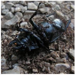
ground-truth information is embedded to the intermediate                 similar features to select similar sub-networks. Though
features during training, and hence the intermediate fea-                different perspectives are emphasized, both loss functions
tures are more suitable to measure the similarity between                describe intrinsic relationships between instances and net-
different samples. The sub-network for instance xi can be                works, and can be simultaneously optimized to get an opti-
described by the channel saliencies, which determine the                 mal solution.
architecture of the network. Note that both the channel                      Based on the channel saliencies of each layer, the
saliencies π l (xi ) and intermediate features F l (xi ) are cor-        dynamic pruning is applied to the given network for
responding to each layer, and thus we can calculate the sim-             different input data separately. Given N different in-
ilarity matrix of channel saliencies T l ∈ RN ×N and simi-               put examples {xi }N             i=1 , the average channel saliencies
larity matrix of features Rl ∈ RN ×N layer-by-layer, where               over different instance are first calculated as π̄ l =
the element T l [i, j] (Rl [i, j]) in the matrix reflect the sim-        {π̄ l [1], π̄ l [2], · · · , π̄ l [cl ]}, where cl is the number of chan-
ilarity between saliencies (features) derived from different             nels in the l-th layer. Then the elements in π̄ l is sorted so
sample xi and xj . Suppose that the classical cosine simi-               that π̄ l [1] ≤ π̄ l [2] ≤ · · · ≤ π̄ l [cl ] and the threshold is
larity [38] is adopted, T l is calculated as:                            set as ξ l = π l [dηcl e], where η is the pre-defined pruning
                                                                         rate and d·e denotes round-off. At inference, only channels
                                π l (xi ) · π l (xj )                    with saliencies larger than the threshold ξ l need to be calcu-
             T l [i, j] =                               ,      (8)
                            kπ l (xi )k2 · kπ l (xj )k2                  lated and the redundant features are skipped, which reduces
                                                                         the computation and memory cost. Based on the threshold
where k · k2 denotes `2 -norm. For intermediate feature
              l   l  l                                                   ξ l derived from the average saliencies π̄ l , the actual prun-
F l (xi ) ∈ Rc ×w ×h in the l-the layer, it is first flattened           ing rate are different for each instances, since the channel
to a vector using the average pooling operation p(·), and                saliency π l (xi ) depends on the input and variant numbers
then the similarity matrix is:                                           of elements are larger than the threshold ξ l . A series of
                           p(F l (xi )) · p(F l (xj ))                   sub-networks with various computational cost are obtained,
          Rl [i, j] =                                     .    (9)       which are intuitively visualized in Figure 8 of Section 5.3.
                        kp(F l (xi ))k2 · kp(F l (xj ))k2

Given the similarity matrices T l and Rl mentioned above, a              5. Experiments
loss function Lsim is developed to impose consistency con-                  In this section, the proposed dynamic pruning method
straint on them, i.e.,                                                   based manifold regularization (ManiDP) is empirically in-
                                    L
                                    X                                    vestigated on image classification datasets CIFAR-10 [22]
                 Lsim (X , W) =           dis(T l , Rl ),     (10)       and ImageNet (LSVRC-2012) [5]. CIFAR-10 contains
                                    l=1                                  60k 32×32 colored images from 10 categories, where
                                                                         50k images are used as the training set and 10k for test-
where X = {xi }N  i=1 and W denote the input data and net-               ing. The large-scale ImageNet (LSVRC-2012) dataset com-
work parameters, respectively, and dis(·, ·) measures the                poses of 1.28M training images and 50k validation im-
difference between the two similarity matrices. Here we                  ages, which are collected from 1k categories. Prevalent
adopt a simple way that compares the corresponding ele-                  ResNet [15] models with different depths and light-weight
ments of the two matrices, i.e., dis(T l , Rl ) = kT l − Rl kF ,         MobilenetV2 [45] are used to verify the effectiveness of the
where k · kF denotes Frobenius norm. In the practical im-                proposed method.
plementation of network training, the similarity matrices are               Implementation Details. For a fair comparison, the
calculated over input data in each mini-batch for efficiency.            pruning rates for all layers in the network are the same fol-
   Combining the adaptive sparsity loss (Eq. (7)), the final             lowing [9]. In the training phase, we increase the pruning
objective function for training the dynamic network is:                  rate from 0 to an appointed value ξ to gradually make the
           N
           X                         L
                                     X                                   pre-trained networks sparse. The coefficient λ0 regulating
     min     Lce (xi , W) + λ(xi ) ·   kπ l (xi )k1                      the weights of sparsity loss is set to 0.005 for CIFAR-10
      W
           i=1                              l=1
                                                              (11)       and 0.03 for ImageNet, empirically. The coefficient γ for
                 + γ · Lsim (X , W),                                     the similarity loss is set to 10 for both two datasets. All
                                                                         the networks are trained using the stochastic gradient de-
where γ is a weight coefficient for the consistency loss                 scent(SGD) with momentum 0.9. For CIFAR-10, the initial
Lsim (X , W). In Eq. (11), the manifold information is si-               learning rate, batch-size and training epochs are set to 0.2,
multaneously excavated from two complementary perspec-                   128 and 300, respectively, while they are 0.25, 1024 and 120
tives, i.e., complexity and similarity. The former imposes               for ImageNet. Standard data augmentation strategies con-
the consistency between instances complexity and sub-                    taining random crop and horizontal flipping are used. For
networks complexity, while the latter induces instances with             CIFAR-10, the images are padded to size 40×40 and then

                                                                     5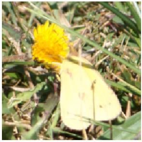
Table 1. Comparison of the pruned ResNet with different methods on ImageNet (ILSVRC-2012). ‘Top-1 Gap’/‘Top-5 Gap’ denotes the
gaps of errors between the pruned models and the baseline models. ‘FLOPs ↓’ is the reduction ratio of FLOPs.
     Model          Method      Dynamic Top-1 Error (%) Top-5 Error (%) Top-1 Gap (%) Top-5 Gap (%) FLOPs ↓ (%)
                    Baseline       -             30.24              10.92               0.0               0.0      0.0
                    MIL [6]        7             33.67              13.06              3.43              2.14     33.3
                   SFP [16]        7             32.90              12.22              2.66              1.30     41.8
                  FPGM [17]        7             31.59              11.52              1.35              0.60     41.8
                   PFP [27]        7             34.35              13.25              4.11              2.33     43.1
   ResNet-18       DSA [39]        7             31.39              11.65              1.15              0.73     40.0
                   LCCN [6]        3             33.67              13.06              3.43              2.14     34.6
                  CGNet [20]       3             31.70                 -               1.46                -      50.7
                    FBS [9]        3             31.83              11.78              1.59              0.86     49.5
                  ManiDP-A         3             31.12              11.24              0.88              0.32     51.0
                  ManiDP-B         3             31.65              11.71              1.41              0.79     55.1
                    Baseline       -             26.69               8.58               0.0               0.0      0.0
                   SFP [16]        7             28.17               9.67              1.48              1.09     41.1
                  FPGM [17]        7             27.46               8.87              0.07              0.29     41.1
                  Taylor [37]      7             27.17                 -               0.48                -      24.2
                   DMC [8]         7             27.43               8.89              0.74              0.31     43.4
   ResNet-34
                   LCCN [6]        3             27.01               8.81              0.32              0.23     24.8
                  CGNet [20]       3             28.70                 -               2.01                -      50.4
                    FBS [9]        3             28.34               9.87              1.85              1.29     51.2
                  ManiDP-A         3             26.70               8.58              0.01               0.0     46.8
                  ManiDP-B         3             27.26               8.96              0.57              0.38     55.3

Table 2. Comparison of the pruned MobileNetV2 with different methods on ImageNet (ILSVRC-2012). ‘Top-1 Gap’/‘Top-5 Gap’ denotes
the gaps of errors between the pruned models and the baseline models. ‘FLOPs ↓’ is the reduction ratio of FLOPs.
      Model           Method      Dynamic Top-1 Error (%) Top-5 Error (%) Top-1 Gap (%) Top-5 Gap (%) FLOPs ↓ (%)
                      Baseline        -            28.20               9.57               0.0                0.0      0.0
                    ThiNet [36]       7            36.25              14.59              8.05               5.02     44.7
                     DCP [62]         7            35.78                 -               7.58                 -      44.7
                    MetaP [34]        7            28.80                 -               0.60                 -      27.7
  MobileNetV2        DMC [8]          7            31.63              11.54              3.43               1.97     46.0
                      FBS [9]         3            29.07               9.91              0.87               0.34     33.6
                    ManiDP-A          3            28.58               9.72              0.38               0.15     37.2
                    ManiDP-B          3            30.38              10.55              2.18               0.98     51.2

cropped to size 32×32. For ImageNet, images with resolu-           reduce substantial computational cost for a given network
tion 224 × 224 are sent to the networks. All the experiments       with negligible performance degradation. For example, the
are conducted with PyTorch [41] on NVIDIA V100 GPUs.               proposed ‘ManiDP-A’ can reduce 46.8% FLOPs ResNet-34
                                                                   with only 0.01% performance degradation. Compared with
5.1. Comparison on ImageNet                                        the SOTA pruning algorithms, our method obtains pruned
    The proposed method is compared with state-of-the-art          networks with less computational cost but lower test errors.
network pruning algorithms on the large-scale ImageNet             The static methods are obviously inferior to ours, e.g., the
dataset. The pruning results of ResNet and MobileNetV2             SOTA method DSA [39] only reduces 40.0% FLOPs and
are shown in Table 1 and Table 2, respectively, where the          obtain a pruned network with 31.39% top-1 error (ResNet-
top-1/top-5 errors of the pruned networks and the reduction        18), while the proposed ‘ManiDP-A’ can achieve lower test
ratios of FLOPs are reported. For dynamic pruning meth-            error (31.12%) with more FLOPs reduced (51.0%). Our
ods, the average FLOPs of the sub-networks over the whole          method also shows superiority to the existing dynamic prun-
test dataset are calculated as computational cost.                 ing methods, e.g., FBS [9] achieves 31.83% top-1 error with
    For ResNet in Table 1, ‘ManiDP-A’ and ‘ManiDP-B’               49.5% FLOPs pruned, which is worse than our method. We
denote two pruned networks with different pruning rates,           can infer that the proposed ManiDP method can excavate
respectively. The competing methods include both SOTA              the redundancy of networks adequately to get compact but
static channel pruning method developed recently ([16, 17,         powerful networks with high performance.
39, 25, 26]) and the pioneering dynamic methods ([9, 6,               To validate the effectiveness of the proposed ManiDP
20]), indicated by 7 and 3 in the table. Our method can            method on light-weight networks, we further compare it

                                                               6
Table 3. Realistic acceleration (‘Realistic Acl.’) and theoretical ac-       Table 4. Comparison of the pruned ResNet with different methods
celeration (‘Theoretical Acl.’) of pruned Networks on ImageNet.              on CIFAR-10.
                                      Theoretical Realistic                   Depth       Method      Dynamic Error (%) FLOPs ↓ (%)
         Model           Method
                                        Acl. (%)       Acl. (%)                          Baseline          -        7.78            0.0
                       ManiDP-A            51.0          35.4                            SFP[16]          7         9.17           42.2
       ResNet-18                                                                        FPGM [17]         7         9.56           54.0
                       ManiDP-B            55.6          40.5
                       ManiDP-A            46.8          32.0                            DSA [39]         7         8.62           50.3
       ResNet-34                                                                20
                       ManiDP-B            55.3          37.4                           Hinge [25]        7         8.16           45.5
                                                                                         DHP [26]         7         8.46           51.8
                       ManiDP-A            37.2          30.4
     MobileNetV2                                                                         FBS [9]          3         9.03           53.1
                       ManiDP-B            51.2          38.5
                                                                                         ManiDP           3         7.95           54.2
with SOTA methods on the efficient MobileNetV2 [45]                                      Baseline          -        7.34            0.0
                                                                                          MIL[6]          7         9.26           31.2
designed for resource-limited devices, and the results are
                                                                                         SFP [16]         7         7.92           41.5
shown in Table 2. Our method also achieves a better                             32
                                                                                        FPGM [17]         7         8.07           53.2
trade-off between network accuracy and computational cost                                FBS [9]          3         8.02           55.7
than the existing methods. For examples, the proposed                                    ManiDP           3         7.85           63.2
‘ManiDP-A’ reduces 37.2% FLOPs of MobileNetV2 with                                       Baseline          -        6.30            0.0
only 0.38% accuracy loss, while the pruned network ob-                                   SFP [16]         7         7.74           52.6
tained by the competing method FBS [9] sacrifices 0.87%                                 FPGM [17]         7         6.51           52.6
accuracy for pruning 33.6% FLOPs. The results show that                                 HRank [28]        7         6.83           50.0
even light-weight networks are over parameterized when                          56       DSA [39]         7         7.09           52.2
exploring redundancy for each instances separately, which                               Hinge [25]        7         6.31           50.0
can be further accelerated by the proposed method and de-                                DHP [26]         7         6.42           50.9
ployed on edge devices.                                                                  FBS [9]          3         6.48           53.6
   The realistic accelerations of the pruned Networks on                                 ManiDP           3         6.36           62.4
ImageNet are shown in Table 3, which is calculated by
                                                                             Table 5. Effectiveness of Excavating Manifold Information. The
counting the average inference time for handling each im-
                                                                             top-1 errors of the pruned networks and the gaps from the base
age on CPUs. The realistic acceleration is slightly less than
                                                                             networks are reported.
the theoretical acceleration calculated by FLOPs, which is                        Model        Complexity Similarity Error / Gap (%)
due to practical factors such as I/O operations (e.g., access-
                                                                                                    7             7         6.88 / 0.58
ing weights of networks), BLAS libraries and buffer switch,                      ResNet-56          3             7         6.61 / 0.31
whose impact can be further reduced by practical engineer-                      (CIFAR-10)          7            3          6.53 / 0.23
ing optimization.                                                                                   3            3          6.36 / 0.06
5.2. Comparison on CIFAR-10                                                                         7             7         28.12 / 1.43
                                                                                 ResNet-34          3             7         27.67 / 0.98
   On the benchmark CIFAR-10 dataset, the comparison                            (ImageNet)          7            3          27.63 / 0.94
between the proposed ManiDP and SOTA channel pruning                                                3            3          27.29 / 0.57
methods are shown in Table 4. Compared with SOTA meth-
ods, a significantly higher FLOPs reduction is achieved by                   larity relationship is empirically investigated in Table 5, in-
our method with less degradation of performance. For ex-                     dicated by 3 and 7. The classification error and the per-
ample, using our method, more than 60% FLOPs of the                          formance gap compared to the base models are reported.
ResNet-56 model are reduced while the test error can still                   Without utilizing the complexity relationship means fixing
achieve 6.36% using ManiDP. Compared to the static meth-                     the trade-off coefficient λ(xi ) between lasso loss and cross-
ods (e.g., HRank [28] with 6.83% error and 50.0% FLOPs                       entropy loss, which obviously increases the error incurred
reduction) and dynamic method (e.g., FBS [9] with 6.48%                      by pruning (e.g., 1.43% vs. 0.94% on ImageNet). The un-
error and 53.6% FLOPs reduction), our method shows no-                       satisfactory performance is due to the improper alignment,
table superiority.                                                           i.e., cumbersome sub-networks may be assigned to sim-
                                                                             ple examples, while complex instances are handled by tiny
5.3. Ablation Studies
                                                                             sub-networks with limited representation capability. For
    Effectiveness of Manifold Information. To maximally                      the similarity relationship, deactivating it (setting coeffi-
excavate network redundancy corresponding to each in-                        cient γ for similarity loss to zero) incurs larger performance
stance, the manifold information between instances is ex-                    degradation (e.g., 1.43% vs. 0.98%), which validates the
plored from two perspectives, i.e., complexity and similar-                  effectiveness of exploring the similarity between features
ity. The impacts of whether exploiting complexity or simi-                   of instances and the corrsponding sub-networks. Thus, ex-

                                                                         7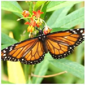
93.7
93.6 7000
93.4 93.6
Accuray (%)
Accuray (%)
93.2 93.5 5000
Number
93.0 93.4
92.8 93.3 3000
92.6
93.2
92.4 1000
92.2 93.1 1.1 1.3 1.7
0 10 4 0.001 0.005 0.01 0.1 0 1.0 5.0 10.0 30.0 50.0 1.5
FLOPs (G)
(a) (b) Figure 5. FLOPs distribution of sub-networks and their corre-
Figure 3. Test accuracies of the pruned ResNet-56 w.r.t. (a) weight sponding input instances on ImageNet.
coefficient λ0 for sparsity loss and (b) coefficient µ for similarity Visualization. Different sub-networks with various
loss. computational costs (i.e., FLOPs) are generated for each
94 instance by pruning different channels. Using ResNet-34
92 0.8
Reduction Rate(%) as the backbone, the FLOPs distribution of different sub-
90
0.6
networks over the validation set of ImageNet are shown in
Accuray (%)
88
86
Figure 8, where x-axis denotes FLOPs and the y-axis is
0.4
84 Accuracy the number of sub-networks. The FLOPs of sub-networks
82 Reduced FLOPs 0.2 varies in a certain range w.r.t. the complexity of instances.
80 Reduced Memory
0.0
Most of the sub-networks own medium sizes and a small
78
0.0 0.2 0.3 0.4 0.5 0.6 0.7 0.8 0.9 quantity of sub-networks activate more/less channels to
Figure 4. The variety of test accuracies and required Memory & handle harder/simpler instances. Some representative im-
FLOPs (ResNet-56) w.r.t. pruning rate η. ages handled by the corresponding sub-networks are also
shown in the figure. Intuitively, a simple example (e.g.,
ploiting both the two perspectives of manifold information ‘bird’ and ‘dog’ in the red frames) that can be correctly pre-
is necessary to achieve negligible performance degradation dicted by a compact network usually contains clear targets,
(i.e., only 0.57% error increase on ImageNet). while images with obscure semantic information (e.g., too
Weight coefficients λ0 and γ. The weights of spar- large ‘orange’ and too small ‘flower’ in the blue frames)
sity loss and similarity loss are controlled by coefficients require larger networks with more powerful representation
λ0 (Eq. (4)) and γ (Eq. 11), whose impact on the final test ability. More visualization results are shown in the supple-
accuracies is shown in Figure 3. A larger λ0 induces more mentary material.
sparsity on channel saliencies, which will have less im-
pact on the network outputs when discarding channels with 6. Conclusion
small saliencies. On the other hand, the sparsity will affect This paper proposes a manifold regularized dynamic
the representation ability of networks and incur accuracy pruning method (ManiDP) to maximally excavate the re-
drop (Figure 3 (a)). Analogous phenomenon exists when dundancy of neural networks. We explore the manifold
varying coefficient γ for similarity loss. The test accuracy information in the sample space to discover the relation-
of the pruned network is improved when increasing γ un- ship between different instances from two perspectives, i.e.,
less it is set to an extremely large value, as the similarity complexity and similarity, and then the relationship is pre-
between different instances is excavated more adequately. served in the corresponding sub-networks. An adaptive
Note that our method is robust to both hyper-parameters and penalty weight for network sparsity is developed to align
works well in a wide range (e.g., range [0.001,0.01] for λ the instance complexity and network complexity, while the
and values around 10.0 for γ), empirically. similarity relationship is preserved by matching the similar-
Memory/FLOPs and accuracies w.r.t. Pruning Rate. ity matrices. Extensive experiments are conducted on sev-
The impact of different pruning rate is shown in Figure 4. eral benchmarks to verify the effectiveness of our method.
When a single instance is sent to the network, the memory Compared with the state-of-the-art methods, the pruned net-
cost for accessing network weights can be reduced as in- works obtained by the proposed ManiDP can achieve better
effective weights do not participate the inference process. performance with less computational cost. For example, our
With a large reduction of computational cost and memory, method can reduce 55.3% FLOPs of ResNet-34 with only
the pruned network can still achieve a high performance. 0.57% top-1 accuracy degradation on ImageNet.
For example, when setting the pruning rare to 0.6% with Acknowledgment. This work is supported by National
73.87% FlOPs and 67.42% memory reduction, the pruned Natural Science Foundation of China under Grant No.
ResNet-56 can still achieve an accuracy of 93.29% (only 61876007, and Australian Research Council under Project
0.41% accuracy drop compared to the original network). DE180101438 and DP210101859.
8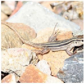
References                                                                       on Computer Vision and Pattern Recognition, pages 1580–
                                                                                 1589, 2020. 1
 [1] Oreste Acuto, Vincenzo Di Bartolo, and Frédérique Michel.
                                                                          [14]   Kai Han, Yunhe Wang, Yixing Xu, Chunjing Xu, Enhua Wu,
     Tailoring t-cell receptor signals by proximal negative feed-
                                                                                 and Chang Xu. Training binary neural networks through
     back mechanisms. Nature Reviews Immunology, 8(9):699–
                                                                                 learning with noisy supervision. In International Conference
     712, 2008. 4
                                                                                 on Machine Learning, pages 4017–4026. PMLR, 2020. 1
 [2] Eulalia Belloc and Raúl Méndez. A deadenylation negative           [15]   Kaiming He, Xiangyu Zhang, Shaoqing Ren, and Jian Sun.
     feedback mechanism governs meiotic metaphase arrest. Na-                    Deep residual learning for image recognition. In Proceed-
     ture, 452(7190):1017–1021, 2008. 4                                          ings of the IEEE conference on computer vision and pattern
 [3] Hanting Chen, Yunhe Wang, Han Shu, Yehui Tang, Chunjing                     recognition, pages 770–778, 2016. 1, 5
     Xu, Boxin Shi, Chao Xu, Qi Tian, and Chang Xu. Frequency             [16]   Yang He, Guoliang Kang, Xuanyi Dong, Yanwei Fu, and
     domain compact 3d convolutional neural networks. In Pro-                    Yi Yang. Soft filter pruning for accelerating deep convolu-
     ceedings of the IEEE/CVF Conference on Computer Vision                      tional neural networks. In Proceedings of the 27th Inter-
     and Pattern Recognition, pages 1641–1650, 2020. 2                           national Joint Conference on Artificial Intelligence, pages
 [4] Hanting Chen, Yunhe Wang, Chang Xu, Chao Xu, and                            2234–2240, 2018. 6, 7
     Dacheng Tao. Learning student networks via feature embed-            [17]   Yang He, Ping Liu, Ziwei Wang, Zhilan Hu, and Yi Yang.
     ding. IEEE Transactions on Neural Networks and Learning                     Filter pruning via geometric median for deep convolutional
     Systems, 2020. 1                                                            neural networks acceleration. In Proceedings of the IEEE
 [5] Jia Deng, Wei Dong, Richard Socher, Li-Jia Li, Kai Li,                      Conference on Computer Vision and Pattern Recognition,
     and Li Fei-Fei. Imagenet: A large-scale hierarchical image                  pages 4340–4349, 2019. 6, 7
     database. In 2009 IEEE conference on computer vision and             [18]   Yihui He, Xiangyu Zhang, and Jian Sun. Channel pruning
     pattern recognition, pages 248–255. Ieee, 2009. 5                           for accelerating very deep neural networks. In Proceedings
 [6] Xuanyi Dong, Junshi Huang, Yi Yang, and Shuicheng Yan.                      of the IEEE International Conference on Computer Vision,
     More is less: A more complicated network with less infer-                   pages 1389–1397, 2017. 1
     ence complexity. In Proceedings of the IEEE Conference               [19]   Geoffrey Hinton, Oriol Vinyals, and Jeff Dean. Distill-
     on Computer Vision and Pattern Recognition, pages 5840–                     ing the knowledge in a neural network. arXiv preprint
     5848, 2017. 2, 6, 7                                                         arXiv:1503.02531, 2015. 1
 [7] Christoph Feichtenhofer, Axel Pinz, and Richard P Wildes.            [20]   Weizhe Hua, Yuan Zhou, Christopher M De Sa, Zhiru Zhang,
     Spatiotemporal multiplier networks for video action recog-                  and G Edward Suh. Channel gating neural networks. In
     nition. In Proceedings of the IEEE conference on computer                   Advances in Neural Information Processing Systems, pages
     vision and pattern recognition, pages 4768–4777, 2017. 1                    1886–1896, 2019. 2, 3, 6
 [8] Shangqian Gao, Feihu Huang, Jian Pei, and Heng Huang.                [21]   Lai Jiang, Mai Xu, Tie Liu, Minglang Qiao, and Zulin Wang.
     Discrete model compression with resource constraint for                     Deepvs: A deep learning based video saliency prediction ap-
     deep neural networks. In Proceedings of the IEEE/CVF Con-                   proach. In Proceedings of the european conference on com-
     ference on Computer Vision and Pattern Recognition, pages                   puter vision (eccv), pages 602–617, 2018. 1
     1899–1908, 2020. 6                                                   [22]   Alex Krizhevsky, Geoffrey Hinton, et al. Learning multiple
 [9] Xitong Gao, Yiren Zhao, Lukasz Dudziak, Robert Mullins,                     layers of features from tiny images. 2009. 5
     and Cheng-zhong Xu. Dynamic channel pruning: Feature                 [23]   Alex Krizhevsky, Ilya Sutskever, and Geoffrey E Hinton.
     boosting and suppression. In International Conference on                    Imagenet classification with deep convolutional neural net-
     Learning Representations, 2018. 1, 2, 3, 5, 6, 7                            works. Communications of the ACM, 60(6):84–90, 2017. 1
[10] Ross Girshick. Fast r-cnn. In Proceedings of the IEEE inter-         [24]   Vadim Lebedev, Yaroslav Ganin, Maksim Rakhuba, Ivan Os-
     national conference on computer vision, pages 1440–1448,                    eledets, and Victor Lempitsky. Speeding-up convolutional
     2015. 1                                                                     neural networks using fine-tuned cp-decomposition. arXiv
[11] Jianyuan Guo, Kai Han, Yunhe Wang, Chao Zhang, Zhaohui                      preprint arXiv:1412.6553, 2014. 1
     Yang, Han Wu, Xinghao Chen, and Chang Xu. Hit-detector:              [25]   Yawei Li, Shuhang Gu, Christoph Mayer, Luc Van Gool,
     Hierarchical trinity architecture search for object detection.              and Radu Timofte. Group sparsity: The hinge between fil-
     In Proceedings of the IEEE/CVF Conference on Computer                       ter pruning and decomposition for network compression. In
     Vision and Pattern Recognition, pages 11405–11414, 2020.                    Proceedings of the IEEE/CVF Conference on Computer Vi-
     1                                                                           sion and Pattern Recognition, pages 8018–8027, 2020. 6,
[12] Jianyuan Guo, Yuhui Yuan, Lang Huang, Chao Zhang,                           7
     Jin-Ge Yao, and Kai Han. Beyond human parts: Dual                    [26]   Yawei Li, Shuhang Gu, Kai Zhang, Luc Van Gool, and Radu
     part-aligned representations for person re-identification. In               Timofte. Dhp: Differentiable meta pruning via hypernet-
     Proceedings of the IEEE/CVF International Conference on                     works. 2020. 6, 7
     Computer Vision, pages 3642–3651, 2019. 1                            [27]   Lucas Liebenwein, Cenk Baykal, Harry Lang, Dan Feldman,
[13] Kai Han, Yunhe Wang, Qi Tian, Jianyuan Guo, Chunjing                        and Daniela Rus. Provable filter pruning for efficient neural
     Xu, and Chang Xu. Ghostnet: More features from cheap                        networks. In International Conference on Learning Repre-
     operations. In Proceedings of the IEEE/CVF Conference                       sentations, 2020. 2, 3, 6

                                                                      9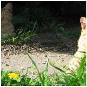
[28] Mingbao Lin, Rongrong Ji, Yan Wang, Yichen Zhang,                     [40] Wonpyo Park, Dongju Kim, Yan Lu, and Minsu Cho. Rela-
     Baochang Zhang, Yonghong Tian, and Ling Shao. Hrank:                       tional knowledge distillation. In Proceedings of the IEEE
     Filter pruning using high-rank feature map. In Proceedings                 Conference on Computer Vision and Pattern Recognition,
     of the IEEE/CVF Conference on Computer Vision and Pat-                     pages 3967–3976, 2019. 1
     tern Recognition, pages 1529–1538, 2020. 7                            [41] Adam Paszke, Sam Gross, Soumith Chintala, Gregory
[29] Shaohui Lin, Rongrong Ji, Chao Chen, Dacheng Tao, and                      Chanan, Edward Yang, Zachary DeVito, Zeming Lin, Al-
     Jiebo Luo. Holistic cnn compression via low-rank decompo-                  ban Desmaison, Luca Antiga, and Adam Lerer. Automatic
     sition with knowledge transfer. IEEE transactions on pattern               differentiation in pytorch. 2017. 6
     analysis and machine intelligence, 41(12):2889–2905, 2018.            [42] Yongming Rao, Jiwen Lu, Ji Lin, and Jie Zhou. Runtime
     1                                                                          network routing for efficient image classification. IEEE
[30] Shaohui Lin, Rongrong Ji, Yuchao Li, Yongjian Wu, Feiyue                   transactions on pattern analysis and machine intelligence,
     Huang, and Baochang Zhang. Accelerating convolutional                      41(10):2291–2304, 2018. 2, 3
     networks via global & dynamic filter pruning. In IJCAI,               [43] Mohammad Rastegari, Vicente Ordonez, Joseph Redmon,
     pages 2425–2432, 2018. 2                                                   and Ali Farhadi. Xnor-net: Imagenet classification using bi-
[31] Shaohui Lin, Rongrong Ji, Chenqian Yan, Baochang Zhang,                    nary convolutional neural networks. In European conference
     Liujuan Cao, Qixiang Ye, Feiyue Huang, and David Doer-                     on computer vision, pages 525–542. Springer, 2016. 1
     mann. Towards optimal structured cnn pruning via genera-              [44] Joseph Redmon, Santosh Divvala, Ross Girshick, and Ali
     tive adversarial learning. In Proceedings of the IEEE/CVF                  Farhadi. You only look once: Unified, real-time object de-
     Conference on Computer Vision and Pattern Recognition,                     tection. In Proceedings of the IEEE conference on computer
     pages 2790–2799, 2019. 1                                                   vision and pattern recognition, pages 779–788, 2016. 1
[32] Chuanjian Liu, Yunhe Wang, Kai Han, Chunjing Xu, and                  [45] Mark Sandler, Andrew Howard, Menglong Zhu, Andrey Zh-
     Chang Xu. Learning instance-wise sparsity for accelerat-                   moginov, and Liang-Chieh Chen. Mobilenetv2: Inverted
     ing deep models. In Proceedings of the Twenty-Eighth In-                   residuals and linear bottlenecks. In Proceedings of the
     ternational Joint Conference on Artificial Intelligence, pages             IEEE conference on computer vision and pattern recogni-
     3001–3007, 7 2019. 1                                                       tion, pages 4510–4520, 2018. 5, 7
[33] Zhuang Liu, Jianguo Li, Zhiqiang Shen, Gao Huang,
                                                                           [46] Pravendra Singh, Vinay Kumar Verma, Piyush Rai, and
     Shoumeng Yan, and Changshui Zhang. Learning efficient
                                                                                Vinay Namboodiri. Leveraging filter correlations for deep
     convolutional networks through network slimming. In Pro-
                                                                                model compression. In Proceedings of the IEEE/CVF Win-
     ceedings of the IEEE International Conference on Computer
                                                                                ter Conference on Applications of Computer Vision, pages
     Vision, pages 2736–2744, 2017. 1, 2, 3
                                                                                835–844, 2020. 1
[34] Zechun Liu, Haoyuan Mu, Xiangyu Zhang, Zichao Guo, Xin
                                                                           [47] Xiu Su, Shan You, Tao Huang, Fei Wang, Chen Qian, Chang-
     Yang, Kwang-Ting Cheng, and Jian Sun. Metapruning: Meta
                                                                                shui Zhang, and Chang Xu. Locally free weight sharing
     learning for automatic neural network channel pruning. In
                                                                                for network width search. arXiv preprint arXiv:2102.05258,
     Proceedings of the IEEE International Conference on Com-
                                                                                2021. 1
     puter Vision, pages 3296–3305, 2019. 6
[35] Yongxi Lu, Abhishek Kumar, Shuangfei Zhai, Yu Cheng,                  [48] Yehui Tang, Yunhe Wang, Yixing Xu, Hanting Chen, Boxin
     Tara Javidi, and Rogerio Feris. Fully-adaptive feature shar-               Shi, Chao Xu, Chunjing Xu, Qi Tian, and Chang Xu. A semi-
     ing in multi-task networks with applications in person at-                 supervised assessor of neural architectures. In Proceedings
     tribute classification. In Proceedings of the IEEE conference              of the IEEE/CVF Conference on Computer Vision and Pat-
     on computer vision and pattern recognition, pages 5334–                    tern Recognition, pages 1810–1819, 2020. 1
     5343, 2017. 1                                                         [49] Yehui Tang, Yunhe Wang, Yixing Xu, Dacheng Tao, Chun-
[36] Jian-Hao Luo, Hao Zhang, Hong-Yu Zhou, Chen-Wei Xie,                       jing Xu, Chao Xu, and Chang Xu. Scop: Scientific con-
     Jianxin Wu, and Weiyao Lin. Thinet: pruning cnn filters                    trol for reliable neural network pruning. arXiv preprint
     for a thinner net. IEEE transactions on pattern analysis and               arXiv:2010.10732, 2020. 1, 2
     machine intelligence, 41(10):2525–2538, 2018. 1, 6                    [50] Yehui Tang, Shan You, Chang Xu, Jin Han, Chen Qian,
[37] Pavlo Molchanov, Arun Mallya, Stephen Tyree, Iuri Frosio,                  Boxin Shi, Chao Xu, and Changshui Zhang. Reborn filters:
     and Jan Kautz. Importance estimation for neural network                    Pruning convolutional neural networks with limited data. In
     pruning. In Proceedings of the IEEE Conference on Com-                     Proceedings of the AAAI Conference on Artificial Intelli-
     puter Vision and Pattern Recognition, pages 11264–11272,                   gence, volume 34, pages 5972–5980, 2020. 2
     2019. 2, 3, 6                                                         [51] Jing Wang, Zhenyue Zhang, and Hongyuan Zha. Adaptive
[38] Hieu V Nguyen and Li Bai. Cosine similarity metric learning                manifold learning. Advances in neural information process-
     for face verification. In Asian conference on computer vision,             ing systems, 17:1473–1480, 2004. 4
     pages 709–720. Springer, 2010. 5                                      [52] Wei Wen, Chunpeng Wu, Yandan Wang, Yiran Chen, and
[39] Xuefei Ning, Tianchen Zhao, Wenshuo Li, Peng Lei, Yu                       Hai Li. Learning structured sparsity in deep neural networks.
     Wang, and Huazhong Yang. Dsa: More efficient budgeted                      In Advances in neural information processing systems, pages
     pruning via differentiable sparsity allocation. In Proceed-                2074–2082, 2016. 2, 3
     ings of the European conference on computer vision, 2020.             [53] Jiaxiang Wu, Cong Leng, Yuhang Wang, Qinghao Hu, and
     6, 7                                                                       Jian Cheng. Quantized convolutional neural networks for

                                                                      10
mobile devices. In Proceedings of the IEEE Conference
on Computer Vision and Pattern Recognition, pages 4820–
4828, 2016. 1
[54] Yixing Xu, Yunhe Wang, Hanting Chen, Kai Han, Chun-
jing Xu, Dacheng Tao, and Chang Xu. Positive-unlabeled
compression on the cloud. arXiv preprint arXiv:1909.09757,
2019. 1
[55] Yixing Xu, Chang Xu, Xinghao Chen, Wei Zhang, Chunjing
Xu, and Yunhe Wang. Kernel based progressive distillation
for adder neural networks. arXiv preprint arXiv:2009.13044,
2020. 1
[56] Zhaohui Yang, Yunhe Wang, Xinghao Chen, Boxin Shi,
Chao Xu, Chunjing Xu, Qi Tian, and Chang Xu. Cars: Con-
tinuous evolution for efficient neural architecture search. In
Proceedings of the IEEE/CVF Conference on Computer Vi-
sion and Pattern Recognition, pages 1829–1838, 2020. 1
[57] Zhaohui Yang, Yunhe Wang, Kai Han, Chunjing Xu, Chao
Xu, Dacheng Tao, and Chang Xu. Searching for low-
bit weights in quantized neural networks. arXiv preprint
arXiv:2009.08695, 2020. 1
[58] Haoran You, Xiaohan Chen, Yongan Zhang, Chaojian Li,
Sicheng Li, Zihao Liu, Zhangyang Wang, and Yingyan Lin.
Shiftaddnet: A hardware-inspired deep network. arXiv
preprint arXiv:2010.12785, 2020. 1
[59] Shan You, Tao Huang, Mingmin Yang, Fei Wang, Chen
Qian, and Changshui Zhang. Greedynas: Towards fast
one-shot nas with greedy supernet. In Proceedings of
the IEEE/CVF Conference on Computer Vision and Pattern
Recognition, pages 1999–2008, 2020. 1
[60] Shan You, Chang Xu, Chao Xu, and Dacheng Tao. Learning
from multiple teacher networks. In Proceedings of the 23rd
ACM SIGKDD International Conference on Knowledge Dis-
covery and Data Mining, pages 1285–1294, 2017. 1
[61] Bo Zhu, Jeremiah Z Liu, Stephen F Cauley, Bruce R Rosen,
and Matthew S Rosen. Image reconstruction by domain-
transform manifold learning. Nature, 555(7697):487–492,
2018. 4
[62] Zhuangwei Zhuang, Mingkui Tan, Bohan Zhuang, Jing Liu,
Yong Guo, Qingyao Wu, Junzhou Huang, and Jinhui Zhu.
Discrimination-aware channel pruning for deep neural net-
works. In Advances in Neural Information Processing Sys-
tems, pages 875–886, 2018. 6
11Label: ship
(a) Complex Instance (a) (b)
Without similarity loss
Label: airplane
(b) Simple instance
(c) (d)
Figure 6. Coefficient λ(xi ) that controls network sparsity for com-
plex and simple instances. With similarity loss
Figure 7. Similarity matrices. (a) Similarity matrix Rl for interme-
7. Supplementary Material diate features without similarity loss. (b) Similarity matrix T l for
channel saliencies without similarity loss. (c) Similarity matrix Rl
7.1. Coefficient λ(xi ) for different instances for intermediate features with similarity loss. (d) Similarity matrix
T l for channel saliencies with similarity loss.
In the training procedure, the coefficient λ(xi ) (Eq. (6)
of the main paper) controls the weight of sparsity loss ac-
cording to the complexity of each instance. Recall that lower point means higher degree of similarity between
λ(xi ) = λ0 · βi C−LceC(xi ,W) ∈ [0, λ0 ] , where λ0 is a two instances). The ResNet-56 model trained with/without
fixed hyper-parameter for all instances. Using ResNet-56 the similarity loss Lsim (Eq. (10) in the main paper) is
as the backbone, the variable parts λ(xi )/λ0 ∈ [0, 1] for used to generate features and channel saliencies for calcu-
complex/simple examples in CIFAR-10 are shown in Fig- lating the similarity between instances randomly sampled
ure 6. λ(xi )/λ0 keeps small for complex examples (e.g., from CIFAR-10. When training dynamic network with-
the vague ‘ship’ in (a)) and then less channels of the pre- out similarity loss Lsim , the similarity calculated by fea-
defined networks are pruned for keeping their representa- tures and that by channel saliencies are very different (Fig-
tion capabilities. When sending simple examples (e.g., clear ure 7 (a), (b)). When using similarity loss (Figure 7 (c), (d)),
‘airplane’ in (b)) to the dynamic network, λ(xi )/λ0 keeps the similarity matrices Rl and T l are more analogous as the
large in most of the epochs, and thus the corresponding sub- similarity loss penalizes the inconsistency between similar-
network becomes sparser continuously as the numbers of it- ity matrices to align the similarity relationship in the two
eration increases. Note that λ(xi )/λ0 changes dynamically spaces.
in the training process. For example, the sparsity weight
automatically decreases in the last few epochs as the cor- 7.3. Visualization of instances with different com-
responding sub-network is compact enough and should pay plexity
more attention to accuracy (Figure 6 (b)), which ensures We sample representative images with different com-
that the models can fit input instances well. plexity from ImageNet and intuitively show them in Fig-
ure 8. From top to bottom, the computational costs of sub-
7.2. Similarity Matrices
networks used to predict labels continue to increase. In-
The similarity matrices Rl for intermediate features and tuitively, simple instances that can be accurately predicted
l
T for channel saliencies are shown in Figure 7, where dif- by compacted networks usually contain clear targets, while
ferent colors denote the degree of similarity (i.e., a yel- the semantic information in complex images are vague and
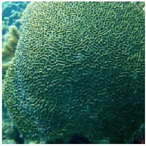
12thus requires larger networks with powerful representation
capability.
Complexity
Figure 8. Images with different complexity on ImageNet. From
top to bottom, the computational costs of sub-networks used to
predict labels continue to increase.
13You can also read