A versatile, linear complexity algorithm for flow routing in topographies with depressions - GFZpublic
←
→
Page content transcription
If your browser does not render page correctly, please read the page content below
Earth Surf. Dynam., 7, 549–562, 2019
https://doi.org/10.5194/esurf-7-549-2019
© Author(s) 2019. This work is distributed under
the Creative Commons Attribution 4.0 License.

         A versatile, linear complexity algorithm for flow routing
                    in topographies with depressions
                                  Guillaume Cordonnier1,2 , Benoît Bovy3 , and Jean Braun3,4
            1 Univ. Grenoble Alpes, 1251 Avenue Centrale Domaine Universitaire, Saint-Martin-d’Hères, France
                   2 Inria
                        Grenoble Rhône-Alpes, 655 Avenue de l’Europe, Montbonnot-Saint-Martin, France
                 3 GFZ German Research Centre for Geosciences, Telegrafenberg 14473, Potsdam, Germany
                             4 University of Potsdam, Am Neuen Palais 10, Potsdam, Germany

                             Correspondence: Guillaume Cordonnier (gllme.cordonnier@gmail.com)

                                  Received: 8 November 2018 – Discussion started: 10 December 2018
                               Revised: 27 March 2019 – Accepted: 12 May 2019 – Published: 19 June 2019

       Abstract. We present a new algorithm for solving the common problem of flow trapped in closed depressions
       within digital elevation models, as encountered in many applications relying on flow routing. Unlike other ap-
       proaches (e.g., the Priority-Flood depression filling algorithm), this solution is based on the explicit computation
       of the flow paths both within and across the depressions through the construction of a graph connecting together
       all adjacent drainage basins. Although this represents many operations, a linear time complexity can be reached
       for the whole computation, making it very efficient. Compared to the most optimized solutions proposed so far,
       we show that this algorithm of flow path enforcement yields the best performance when used in landscape evo-
       lution models. In addition to its efficiency, our proposed method also has the advantage of letting the user choose
       among different strategies of flow path enforcement within the depressions (i.e., filling vs. carving). Furthermore,
       the computed graph of basins is a generic structure that has the potential to be reused for solving other problems
       as well, such as the simulation of erosion. This sequential algorithm may be helpful for those who need to, e.g.,
       process digital elevation models of moderate size on single computers or run batches of simulations as part of an
       inference study.

1   Introduction                                                     den, unrealistic jump in computing discharge. Flow routing
                                                                     is often corrected by filling depressions (e.g., Jenson and
Finding flow paths on a topographic surface represented as           Domingue, 1988), carving channels through artificial sills
a digital elevation model (DEM) is a very common task that           (Rieger, 1998), or by using hybrid breaching-filling tech-
is required by many applications in domains such as hydrol-          niques (Lindsay, 2016).
ogy, geomorphometry, soil erosion, and landscape evolution              Although not having a linear time complexity, the most
modeling, and for which various algorithms have been pro-            recent algorithms of depression removal – e.g., the Priority-
posed for either gridded DEMs (e.g., O’Callaghan and Mark,           Flood algorithm and its variants (Barnes et al., 2014a; Zhou
1984; Jenson and Domingue, 1988; Quinn et al., 1991; Tar-            et al., 2016; Wei et al., 2018) – have been optimized so that
boton, 1997) or unstructured meshes (e.g., Jones et al., 1990;       they can be used efficiently on large datasets. To increase per-
Banninger, 2007).                                                    formance for very large datasets, further optimization efforts
   Closed depressions may arise in DEMs because they are             have been focused primarily on rather complex, parallel vari-
real topographic features or result from interpolation error         ants of these algorithms (Barnes, 2016; Zhou et al., 2017).
during DEM generation or its lack of resolution. These spu-             Yet, in some applications flow path enforcement still re-
rious local minima need to be resolved because they disrupt          mains the main bottleneck. This is for example the case
flow routing, produce hydrologically unrealistic results, or         in many landscape evolution models (LEMs) simulating an
introduce artificial singularities that may result from a sud-

Published by Copernicus Publications on behalf of the European Geosciences Union.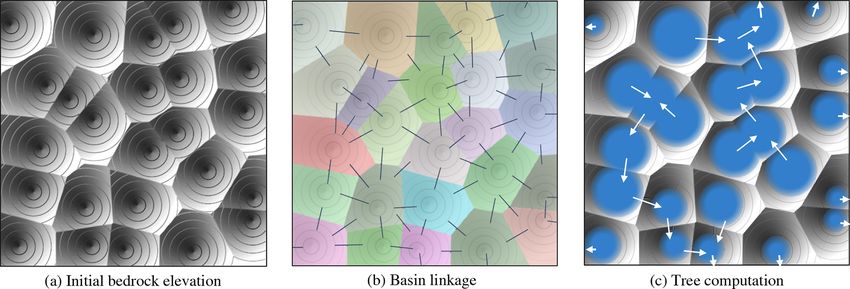
550                                                                       G. Cordonnier et al.: Linear complexity flow routing

evolving topography (see Tucker and Hancock, 2010, for a           of the neighbors of n and is defined as Donors(n) = {k ∈
review) and that rely on flow routing to compute erosion           Nb(n), s.t. rcv(k) = n}. We set rcv(n) = ∅ when n is a sin-
rates. To produce realistic results, flow path enforcement is      gular node: it corresponds to either a user-defined boundary
often applied many times, i.e., at each simulation time step       node (e.g., a node on the domain boundary) or a local mini-
(Fig. 1), even when this eventually becomes irrelevant as the      mum in the topography, i.e., a node inside the domain where
modeled erosional processes usually tend to remove depres-         all of its neighbors have a higher elevation, and correspond to
sions rather than deepen or add new ones (Braun and Willett,       either a pit or a flat-bottomed depression in Lindsay (2016)
2013). Furthermore, LEMs are also used as forward models           terminology.
in sensitivity analyses and/or inferences on the parameters           We propose an algorithm that updates the receivers of a
that control erosional processes, which often require running      subset of N such that the flow is never trapped in local min-
a large number of models to adequately explore the param-          ima. This algorithm primarily aims at resolving local min-
eter space. Parallel flow routing and hydrological correction      ima in the context of flow routing and thus leaves the eleva-
algorithms do not help much here, as grid-search and/or sam-       tion of the nodes unchanged. Hence it breaks the previously
pling methods (e.g., Sambridge, 1999) are generally easier to      introduced definition of a flow receiver: the new receivers
implement and more effective to execute in parallel. Highly        assigned by the algorithm generally produce some localized
optimized, sequential algorithms are still needed in this case.    “upslope flow”. While this seems unnatural and may not be
   We have developed a new method of flow enforcement that         wanted, the data structures used by the algorithm provide
is based on the explicit building of a graph of drainage basins    enough information to efficiently address this issue later de-
(possibly encompassing depressions) and the computation of         pending on the application, which is beyond the scope of this
the flow paths both within and across those basins. This idea      work. Still, the algorithm ensures that the updated flow rout-
was first introduced in a Computer Graphics implementation         ing stays consistent across the whole topography by respect-
of the stream power law (Cordonnier et al., 2016), but with        ing the following properties for each node n of the topogra-
a sub-optimal complexity. Although this approach may ap-           phy.
pear naive at first glance, we have improved it by using fast
algorithms of linear complexity at each step of the proce-          1. There exists a single boundary node b (not a local min-
dure, which now makes the whole computation very efficient.            imum), and a unique flow path from n to b. The flow
Not only does this method enable the use of a wide range               path is defined as the set of nodes P = (n, rcv(n),
of techniques of flow enforcement within the closed depres-            rcv(rcv(n)), . . ., b).
sions (e.g., depression filling, channel carving, or more ad-       2. This flow path does not contain any cycle; i.e., each
vanced techniques), but it also provides generic data struc-           node appears only once in P .
tures that could potentially be reused for solving other prob-
lems like modeling the behavior of erosion–deposition pro-          3. The receivers defining P are chosen such that it satisfies
cesses within those depressions.                                       properties 1 and 2, and minimizes the energy E, defined
   After a detailed presentation of the different steps of the         as
method, we will show in the sections below through some
results how our algorithm behaves and performs compared to
existing solutions of flow path enforcement. We will finally            X
                                                                   E=    Ei .                                                 (1)
discuss the assets and limitations of our method, with some
                                                                        i∈P
focus on landscape evolution modeling applications.
                                                                   As a first approximation, we set Ei = zi (the altitude of the
                                                                   node). We will discuss later the special case of nodes under
2   Algorithm                                                      water level.
                                                                      Our method is essentially based on the computation of a
The input of the algorithm is a topography T = (N , E),            graph connecting adjacent drainage basins. We define a basin
where N is a set of nodes and E is a set of edges that link        as the set of all nodes that flow toward the same singular node
pairs of neighbor nodes. A node n is given a horizontal po-        (Fig. 2b). A basin is either a boundary basin or an inner basin
sition pn and a vertical elevation zn . A topography may for       depending on whether the singular node is a boundary node
example result from a triangulation or correspond to a regu-       or a local minimum.
lar grid of four-connectivity (i.e, four neighbors per nodes) or      To better explain the problem that we want to solve, we
eight-connectivity (i.e., also including diagonal neighbors).      consider a filled topography as the result of an ideal physi-
We follow the conventions of Braun and Willett (2013) to           cal process where a perfectly fluid material has been poured
define flow paths on the topography: each node n is given (1)      onto an impermeable ground and stabilized at steady state.
a single flow receiver, rcv(n), which corresponds to that of       For a node n, we define as water level (wn ) the elevation
its (strictly) downslope neighbors having the steepest slope,      of the fluid surface, and as a spill any node s such that
and (2) a set of flow donors, Donors(n), which is a subset         ∃d ∈ Donors(s) | wd = ws and zs > wrcv(s) . Note that for a

Earth Surf. Dynam., 7, 549–562, 2019                                                   www.earth-surf-dynam.net/7/549/2019/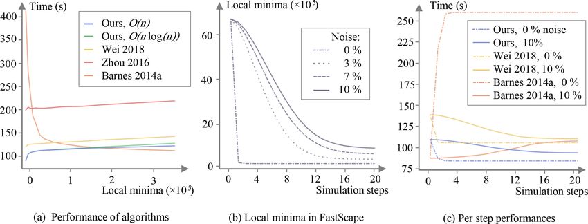
G. Cordonnier et al.: Linear complexity flow routing 551
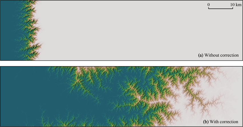
Figure 1. Simulation of the evolution of an escarpment over 70 time steps of 1000 years each and on a 1024 × 256 regular grid, using the
FastScape model (Braun and Willett, 2013, see also Sect. 3 below). The grid nodes of the leftmost column (boundary nodes) have a fixed
elevation while the initial elevation of the other nodes corresponds to a 500 m high flat surface with small random perturbations. Using the
same set of model parameters, simulation results are shown (a) without and (b) with correction of flow routing in local depressions at each
time step. As illustrated, flow path disruptions in (a) cause a much slower migration of the escarpment, while the topography predicted in
(b) is usually considered more realistic, especially under temperate or humid climates.
flow routing observing the aforementioned properties, the 1. Compute the basins and link all pairs of adjacent basins
water level can be computed as wn = max(wrcv(n) , zn ). We (Fig. 2b).
also use the term depression from Lindsay (2016) terminol-
ogy, and we define it with respect to a basin B as a subset of 2. Select only some of the basin links computed at the pre-
nodes of B under water level, characterized by wn = wrcv(n) . vious stage and orient them such that the flow is routed
Note that the water level of a boundary basin corresponds to consistently across adjacent basins, from inner basins
the elevation of its associated boundary node so that it con- toward the boundary basins (Fig. 2c). This operation is
tains no depression. In the case of nested depressions, the not trivial: an optimal selection needs a global knowl-
water level of a basin may be higher than the elevations of edge of the whole basin graph. To do so, we use an
all its nodes, which means that the spill does not always be- algorithmic structure: a minimum spanning tree of the
long to B. basin graph. We propose here two algorithms, a sim-
The energy of the nodes should be changed to Ei = wi , but ple one with O(n log n) complexity, and a more complex
as described later, one may choose various routing strategies one with O(n) complexity.
inside the depressions depending on the application. There-
fore, we allow any path within depressions by setting Ei to 3. Update the flow receivers. Using the links selected at the
zero inside them, and keeping Ei = zi elsewhere. previous stage, we update (only some of) the receivers
One may break the problem of flow path enforcement to enforce the flow both within and across inner basins
down to three smaller problems: find the spill of each de- so that it is ensured to finally reach the boundary basins
pression, force the flow within the depressions to be routed and their associated boundary nodes. We propose three
toward their respective spill, and ensure that the flow through different methods (one may choose a method over an-
the spills is properly routed into adjacent basins. The pro- other depending on the specific problem to solve).
posed algorithm addresses this problem in an explicit manner
and can be divided into three main stages. Each of these stages processes the whole DEM, and as
such are run only once for a given topography. They are each
detailed in the next sections.
www.earth-surf-dynam.net/7/549/2019/ Earth Surf. Dynam., 7, 549–562, 2019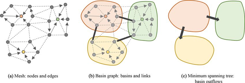
552                                                                                G. Cordonnier et al.: Linear complexity flow routing

Figure 2. Illustration of the inputs and the first steps of the proposed flow routing algorithm. (a) The input topography is defined on top of a
mesh by a set of nodes and edges. A single edge is selected for each node, it connects the node to its flow receiver, i.e., its neighbor with the
steepest slope. Nodes with no receiver are local minima (colored in the figure). (b) All the nodes that flow to a same local minimum belong
to the same basin. A graph of basins is created by connecting together adjacent basins with links, which are materialized on the mesh by
edges representing the passes, i.e., the crossings of lowest elevation that connect each pair of basins (black thick arrows). (c) Some of the
links are selected by computing a minimum spanning tree and the corresponding passes are oriented in the direction of the flow across the
basins (unidirectional arrows). This structure is then used to update the flow receivers so that the flow reaches the domain boundaries without
being interrupted.

2.1   Basin computation and linkage                                        2.2   Flow routing across adjacent basins
                                                                           This second stage tackles the problem of selecting the right
This first stage consists in first assigning a basin identifier,           subset of links so that we obtain consistent flow paths on the
basin_id(n), to each node n of the topography. The identifiers             basin graph. To illustrate the proposed solution, let us start
are added sequentially by starting at singular nodes and pars-             from an inner basin. If it is filled with water, the water level
ing the nodes using a depth-first traversal in the direction of            will rise until it finds a pass where water eventually pours
the donors (see Appendix A1). The case of flat-bottomed de-                into another, adjacent basin. The associated link is then called
pressions does not require any particular treatment: all nodes             the outflow of the basin. Hence, routing the flow across the
within flat areas are singular nodes and therefore are each                basins consists in connecting all outflows such that the re-
assigned a unique basin identifier.                                        sulting flow paths, from inner basins to the boundary basins,
   Then, the links connecting all pairs of adjacent basins are             have the same properties as stated above; i.e., those paths are
retrieved. To each link also corresponds an edge of the to-                unique, contain no cycle, and minimize the energy needed to
pography, here called a pass, which represents the crossing                reach the boundary basins.
of lowest elevation between the two basins. For example,                      If we add to the basin graph a virtual basin (let us call it ex-
the link L = (B1 , B2 ) connects the basins B1 and B2 and                  ternal basin) to which we link all the boundary basins (i.e.,
has the corresponding Pass(L) = (n1 , n2 ), where n1 ∈ B1 and              the external basin may be viewed as a bucket collecting all
n2 ∈ B2 and where the chosen (n1 , n2 ) minimizes zpass(L) =               the flow that leaves the domain), then we can represent the
max(zn1 , zn2 ). We define a single procedure to retrieve both             connected outflows using a specific algorithmic structure: a
the links and their pass (see Appendix A2). This procedure                 tree. More specifically, a basin tree is a tree that satisfies the
parses each edge of the topography: if the two nodes of the                properties above: it actually corresponds to a minimum span-
current edge each have different basin identifiers, then (1) it            ning tree of the basin graph, i.e., a subset of the basin graph
adds a new link if no link has been already set for these two              resulting from a selection of the links so that the following
basins, and (2) it sets or maybe updates the pass of that link             energy is minimized:
with the current edge.                                                              X
   The sets of basins B and the set of retrieved links L both              Etree =      ∈ Ozpass(L) ,                                      (2)
                                                                                     L
define a basin graph. It is worth noting that, at this stage,
the links and passes are not oriented and that only one link                 where O is the set of selected links (or the set of outflows)
and pass are stored for two adjacent basins. The procedure                 and zpass(L) is the elevation of their respective passes.
described above runs sequentially and will not add the link                  We propose two algorithms for the computation of a min-
(B2 , B1 ) if it already added the link (B1 , B2 ).                        imum spanning tree. Kruskal’s algorithm is very generic and

Earth Surf. Dynam., 7, 549–562, 2019                                                             www.earth-surf-dynam.net/7/549/2019/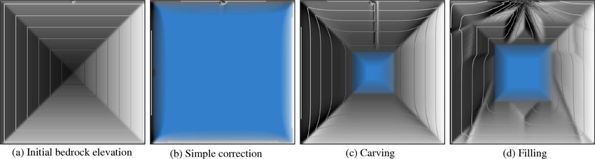
G. Cordonnier et al.: Linear complexity flow routing                                                                           553

simple with a log-linear complexity. We also propose a sec-         The key intuition behind the algorithm proposed in Mareš
ond algorithm, which leverages the planar nature of the basin       (2002) is that at least half of the vertices of a planar graph
graph to reach a linear complexity.                                 have at most eight neighbors. The algorithm is then an adap-
                                                                    tation of another classical algorithm, named Boruvka’s algo-
                                                                    rithm (Boruvka, 1926); see Algorithm 2 for more details. The
                                                                    O(N) complexity comes from the fact that at each step of the
                                                                    outer loop, we parse
                                                                                       P and remove at least half of the nodes
                                                                    of the graph, and N + N/2 + · · · + 1 < 2N. As the num-
                                                                    ber of grid nodes n > N , the complexity of this algorithm
                                                                    is bounded by O(n). As demonstrated by Mareš (2002), the
                                                                    limit of eight neighbors for the selection of a basin in the in-
                                                                    ner loop is critical in halving the number of edges at each
                                                                    iteration of the outer loop and thus in obtaining a linear time
                                                                    complexity.

2.2.1   Kruskal’s algorithm

Kruskal’s algorithm (Kruskal, 1956) is one of the most clas-
sical algorithms used for computing minimum spanning trees
and is known to have a O(m log m) complexity, where m
is the number of links. The number of links being always
bounded by a linear function of the number n of nodes in the
grid (Euler formula), using this algorithm induces a global
upper bound of O(n log n) on the complexity of our solu-
tion. This algorithm uses a union–find structure to store and
merge equivalence classes of objects (see Algorithm 1). The
idea here is to parse all links L ∈ L sorted by increasing ele-
vation zpass(L) , progressively grouping each pair of basins as
a larger, virtual one (equivalence class). All subsequent paths        A special case may arise when the basin graph is computed
between basins within this equivalence class are discarded to       from a grid of eight-connectivity. In this case, the edges of
prevent loops. The union–find data structure has three opera-       the graph may cross each other due to the diagonal connec-
tions:                                                              tivity, possibly making the basin graph not perfectly planar.
                                                                    This is, however, rather unlikely as it implies that two passes
MakeSet Create an equivalence class containing a single el-         connecting different basins are found on the two diagonals
   ement.                                                           connecting four adjacent nodes of the grid. Furthermore, this
                                                                    issue does not impact the correctness of the algorithm. Only
Union Merge two equivalence classes.                                the linear complexity is not formally proven. Because it is
                                                                    not planar, the case of an eight-connectivity grid would fall
Find Get the equivalence class of an object.
                                                                    in the second category mentioned by Mareš (2002) of graphs
   The optimal implementation of the union–find structure           closed on graph minor. We have validated this experimentally
provides a O(α(N)) complexity for these operations, where           by randomly computing minors of differently sized eight-
N is the number of elements in the structure (i.e., here the        connected graphs. We found an edge density of 4, imply-
number of basins) and α is the inverse Ackermann function           ing that half of the basins in the basin graph are linked to at
whose complexity is lower than O(log N ). This however re-          most 16 adjacent basins (and not eight as for planar graphs) at
quires first sorting the links by increasing weight (i.e., by the   any step of the algorithm. Therefore, we have demonstrated
elevation of their respective passes), which finally yields a       the linear complexity for eight-connected graphs experimen-
O(m log m) complexity for the whole computation.                    tally, although future work is needed to prove this in a formal
                                                                    framework.
2.2.2   Planar graphs
                                                                    2.3   Updating flow receivers
The problem of finding the minimum spanning tree is known
to have a O(N) complexity when the graph is planar (Mareš,          The basin tree obtained at the previous stage must be oriented
2002). A planar graph is a graph which can be embedded in a         before routing the flow from inner basins to the boundary
plane such that none of its edges cross another one. The basin      basins. This is achieved by traversing the tree in the reverse
graph described in Sect. 2.1 is an example of a planar graph.       order (i.e., starting from the boundary basins) and labeling

www.earth-surf-dynam.net/7/549/2019/                                                     Earth Surf. Dynam., 7, 549–562, 2019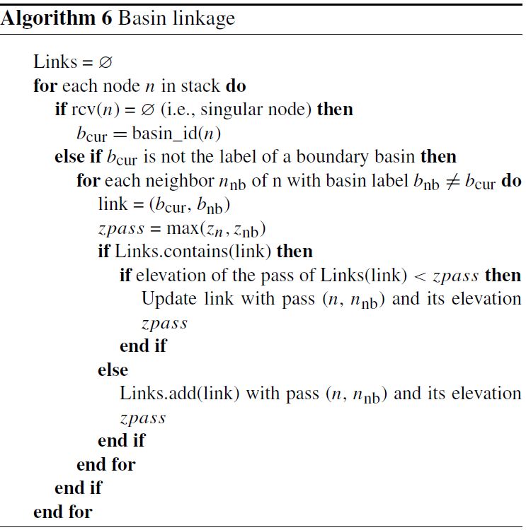
554                                                                         G. Cordonnier et al.: Linear complexity flow routing

the two nodes of each pass, one as nin (incoming flow) and           between a node and nout . This function does not yield the
the other one as nout (outgoing flow). Depending on their el-        perfect path patterns that one would obtain by including ob-
evation, either nin or nout is the spill node of the correspond-     stacles in the computation of the Euclidean distance on a reg-
ing basin.                                                           ular grid, but it is simple and efficient while being accurate
   The last stage then consists in updating the flow receivers       enough. We prefer this method over a simple breadth-first
so that any flow entering an inner basin is ensured to leave the     search, which depends on the order in which neighbors are
basin through nout . The most straightforward solution would         visited and which leads to more pronounced straight lines af-
be to only update the receiver of each local minimum p so            ter erosion, due to the four- or eight-connectivity.
that rcv(p) = nout . Note that if nin has a higher elevation than
nout , then two receivers must be updated: rcv(nin ) = nout and
rcv(n) = nin . This very simple solution ensures topological
continuity of the flow but does not preserve its spatial conti-
nuity. We therefore propose two other, more realistic meth-
ods: one similar to depression filling and another similar to
depression carving. Note that we use carving and filling as
metaphors as our algorithm only changes the flow graph con-
nectivity without altering elevation values. For each of the
variants, the donors and stack structures need to be updated
to reflect the changes in the receivers.

2.3.1   Depression carving
The idea here is to mimic the effect of a river carving a nar-
row trench between the bottom of the depression and the
spill: a new, single path is computed from the local mini-
mum to the pass. In fact, the most direct path is already de-
fined by the flow receivers that were computed initially, but
it is in the reverse order, i.e., from the pass to the local mini-   3   Results
mum. Hence, it is trivial to follow this path and progressively
revert the receivers until the local minimum is reached (see         Our algorithm is run under different settings to illustrate
Algorithm 3).                                                        its behavior and compare it with some other state-of-the-
                                                                     art methods. Most of the examples below are shown within
                                                                     the context of landscape evolution modeling, using a sim-
                                                                     ple model of block uplift vs. channel erosion by the stream
                                                                     power law. This model simulates the evolution of the topo-
                                                                     graphic surface z, which can be written as follows:

                                                                     ∂z
                                                                        = U − K Am (∇z)n ,                                       (3)
                                                                     ∂t

                                                                     where U is the uplift rate, A is the drainage area (a surro-
                                                                     gate for water discharge), ∇z the local topographic gradient,
2.3.2   Depression filling
                                                                     and K, m, and n are the parameters of the stream power law.
Unlike the previous method, we update here the receivers as          The latter is solved numerically on a 2-D regular grid using
if the depressions were completely filled by some material.          an implicit scheme of linear complexity (see the FastScape
We define a procedure that starts at a pass and then progres-        algorithm described in Braun and Willett, 2013). In particu-
sively parses all neighbor nodes in a breadth-first order as         lar, the local gradient ∇z is chosen as the slope between the
long as these are below water level, at the same time updating       eroded node and its receiver (forced to 0 if its value is nega-
the receiver of the current parsed node as being one among           tive in order to avoid erosion artifacts in the case of “upslope
its neighbors that has already been parsed (see Algorithm 4).        flow” caused by updated receivers). We choose this algorithm
We repeat this procedure for all depressions by traversing the       which is particularly well suited to our flow routing method,
basin tree from the boundary basins to the most inner ones so        although some discussion on the limits of this algorithm can
that accurate water level values can be computed during the          be found in Campforts and Govers (2015) for steep topog-
procedure. Receivers are chosen according to a cost func-            raphy. As common settings, we use K = 7 × 10⁻⁴ m0.2 yr−1 ,
tion that we define here as the minimal Euclidean distance           m = 0.4, and n = 1. Grid spacing is 100 m in both directions.

Earth Surf. Dynam., 7, 549–562, 2019                                                     www.earth-surf-dynam.net/7/549/2019/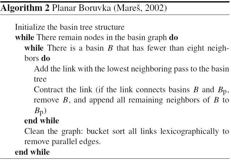
G. Cordonnier et al.: Linear complexity flow routing                                                                                 555

Figure 3. Our algorithm of flow enforcement run on a synthetic case. (a) Hillshade and contour plot of the input topography with apparent
depressions. (b) Basins (areas of unique, random colors) and all passes connecting adjacent basins (thin black lines). (c) Flow directions
across the basins (white arrows), as resulting from the computation of a minimum spanning tree from the basin graph, and water level (blue
areas) after some erosion is applied to the input topography.

3.1   Illustration of the algorithm                                    A single time step of 5000 years of erosion only (no uplift) is
                                                                       performed using each of the strategies described in Sect. 2.3.
The behavior of our algorithm of flow path enforcement is
best illustrated using a simple synthetic topography as in-            Simple correction. In this specific case, the algorithm up-
put. A set of 25 local minima is sampled on a regular grid                 dates the receivers of only three nodes: (1) one of
of 500 × 500 nodes and the elevation of the topographic sur-               the neighbors of the boundary node, which here corre-
face is locally computed as a fixed proportion of the distance             sponds to the spill of the closed depression, (2) one of
to the nearest local minimum (Fig. 3a). The first step of the              the neighbors of the spill that, together with the spill,
algorithm delineates the basin of each local minimum and                   forms the pass connecting the depression to the bound-
finds all possible connections (links) between the basins, lo-             ary node, and (3) the local minimum at the bottom of the
cated at the lowest pass between each pair of adjacent basins              depression. The new assigned receivers are for (1) the
(Fig. 3b). Then, a minimum spanning tree is computed from                  boundary node itself, (2) the spill, and (3) the other
the graph of these links to find the path of minimum energy                node of the pass. We can see in Fig. 4b that this strat-
that would allow the water to leave the basins (white arrows               egy does not allow channel erosion to propagate much
in Fig. 3c). The flow receivers can then be updated by using               from the boundary node into the closed depression. In
the edges of this basin tree. The updated receivers are in turn            fact, drainage area values close to the boundary node
used by the FastScape algorithm to slightly erode the basin                are high enough to trigger erosion but the low values
boundaries during one time step of 100 years. The result is                of drainage area in the vicinity (within the depression)
shown as well as the final water level in Fig. 3c.                         prevent further propagation of the erosion wave.
                                                                       Depression carving. Unlike the former strategy and as ex-
3.2   Effect of flow path enforcement strategies on eroded                 pected, Fig. 4c shows that the depression carving strat-
      topographies                                                         egy allows erosion to propagate toward the local mini-
Figure 1 already shows the effect of flow path enforcement                 mum along a narrow and deep trench.
vs. no enforcement on the evolution of an escarpment under
                                                                       Depression filling. Using the depression filling strategy,
active erosion processes. A second set of experiments, shown
                                                                           flow receivers are updated over a large area of the de-
in Fig. 4, illustrates the impact that the different strategies
                                                                           pression as if the water surface was replaced by a very
of flow receiver updating have on the evolution of the to-
                                                                           gentle slope toward the spill. As a result, erosion affects
pographic surface under the action of channel erosion. The
                                                                           a great part of the modeled domain, with the emergence
input synthetic topography is defined on a 100 × 100 regu-
                                                                           of a star-like pattern centered at the spill (Fig. 4d). The
lar grid and looks like an inverted pyramid with 45◦ regular
                                                                           number and disposition of the branches of the star are
slopes, forming a single, big depression (Fig. 4a). The node
                                                                           due to the grid eight-connectivity used here.
at the middle of the top boundary is the only node that is not
part of the depression: it has the same elevation as the node            Choosing one strategy over another greatly depends on the
at the center of the grid and it is defined as a boundary node.        specific application. For example, the simple correction strat-

www.earth-surf-dynam.net/7/549/2019/                                                          Earth Surf. Dynam., 7, 549–562, 2019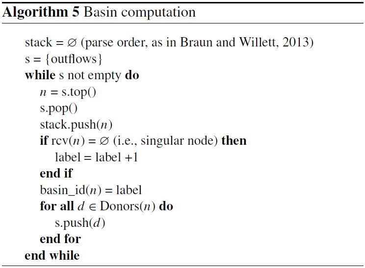
556                                                                              G. Cordonnier et al.: Linear complexity flow routing

Figure 4. Demonstration of the effect of flow path enforcement on erosion, using different strategies of flow receivers “correction” within
inner basins. (a) Hillshade and contour plot of the initial topography. (b), (c) and (d) Hillshade and contour plot of the topography obtained
after running a single time step of 5000 years with channel erosion only (no uplift), with flow receivers updated using each of the different
strategies described in Sect. 2.3. Water level is shown in blue, and is computed by propagating the spill elevation while parsing the nodes in
the upstream order (based on updated donors).

egy may be acceptable if one assumes that no erosion could               most efficient when the number of local minima is large (see
happen in depressions below the water level. However, in-                Sect. 4). While being the most optimized sequential variant
terrupted drainage area patterns within the depressions may              that has been proposed so far, the Wei et al. (2018) variant
be problematic when used with erosion algorithms like the                fills the depressions with perfectly flat surfaces and thus has
FastScape model, which uses an implicit time scheme for                  to be combined with a flat resolution algorithm – we use
solving the stream power law but still treats drainage area              here an optimal O(n) algorithm proposed by Barnes et al.
explicitly, resulting in too slow opening of the closed depres-          (2014b). We apply the same treatment to the Zhou et al.
sions by erosion. The depression carving or depression fill-             (2016) variant. All variants fill the depressions by directly
ing strategies generally yield better results in the latter case.        updating the elevation values on the grid. To ensure proper
These two strategies have, however, contrasting behaviors                comparison with our algorithm, we thus need to run them on
and choosing one or the other will depend on several criteria            a temporary copy of the elevation values before computing
such as the size (i.e., depth vs. volume) of the depressions.            the flow receiver for each node of the grid. With our algo-
                                                                         rithm being optimized for a sequential usage, we chose not
                                                                         to compare it to the parallel versions of Barnes (2016) and
3.3   Performances                                                       Zhou et al. (2017). Both the algorithms and the benchmarks
To assess the performance of our algorithm, we have run                  are implemented using the C++ language. For the state-of-
multiple benchmarks under various settings. Although these               the-art algorithms, we reuse the implementations available
benchmarks mostly take place in the framework of landscape               in the RichDEM library v2.2.9 (Barnes, 2018). The bench-
evolution modeling, they provide results that may be useful              marks where computed on an Intel Xeon Silver 4110 CPU
in other applications too. Note that for better readability, we          (2.1 GHz, 32.0 Go RAM). We used Microsoft Visual Studio
present here only the results from benchmarks applied to a               compiler with fast optimization options. Note that because of
fixed grid of 16 384 × 16 384 nodes. We obtain consistent re-            the differences in the design/implementation used in Rich-
sults for other grid sizes.                                              DEM vs. our code, the benchmarks presented here should be
   We have run benchmarks for our algorithm – including                  seen as an illustration of the theoretical complexities of the
the two variants for computing the minimum spanning tree                 algorithm variants rather than a strict comparison of their ac-
but considering only the depression filling strategy – as well           tual performances.
as for three other state-of-the-art algorithms of local minima               In a first set of benchmarks, we create an input topography
resolution, respectively proposed by Barnes et al. (2014a),              by running the FastScape model (starting from an initial flat
Zhou et al. (2016), and Wei et al. (2018). All three of those            surface with small random perturbations) until steady state is
algorithms fill the depressions using improved variants of               reached (the uplift rate is set to 5 × 10⁻³ m yr−1 ), and then
the Priority-Flood algorithm that reduce the number of nodes             by lowering the elevation of an arbitrary number of nodes
processed by a priority queue. The Barnes et al. (2014a) vari-           down to 10−5 m below their lowest neighbors. Those nodes
ant used here, i.e., Priority-Flood+, is only slightly opti-            are chosen randomly on even rows and columns to make sure
mized but has the advantage of filling the depressions with a            that we obtain the same number of local minima in the input
nearly flat surface so that flow directions can be determined.           topography. Note that each generated basin has a size of at
Interestingly, the simplicity of this first version makes it the         most nine cells, which allows for a fine control on the cumu-

Earth Surf. Dynam., 7, 549–562, 2019                                                           www.earth-surf-dynam.net/7/549/2019/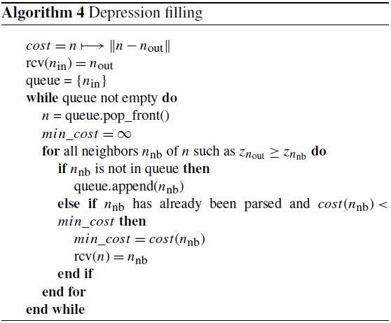
G. Cordonnier et al.: Linear complexity flow routing                                                                                          557

Figure 5. Results from benchmarks assessing the performance of our algorithm for local minima resolution – including both O(n log n)
Kruskal’s and O(n) Mareš’ variants for computing the minimum spanning tree, compared to three other solutions based on variants of the
Priority-Flood depression filling algorithm proposed by Barnes et al. (2014a), Zhou et al. (2016), and Wei et al. (2018). See text for more
details about the setup of these benchmarks. (a) Execution time measured for local minima resolution applied once to a synthetic input
topography vs. total number of local minima generated in the input topography. (b) Evolution of the number of local minima detected
in the topography obtained at each of the first 20 time steps of a FastScape model run. Each curve corresponds to a given magnitude of
random perturbations added to produce spatially variable uplift rates (magnitude values are relative to a fixed uplift rate of 5×10⁻³ m yr−1 ).
(c) Execution time measured for local minima resolution at each time step, with either spatially uniform or variable uplift rates (i.e., a relative
noise magnitude of either 0 % or 20 %). The blue curves refer to our algorithm using the O(n) variant for computing the minimum spanning
tree.

lative size of the depressions. Figure 5a shows the execution                  In a second set of benchmarks, we analyze the perfor-
times of our algorithm vs. state-of-the-art algorithms for an               mances of the algorithms for local minima resolution through
increasing number of local minima. We can see that in these                 full simulations of landscape evolution. We run the FastScape
settings our algorithm (both variants for the computation of                model over 20 time steps of 10 000 years each, starting from
the minimum spanning tree) globally outperforms the state-                  a flat topography with small random perturbations (thus con-
of-the-art solution of Wei et al. (2018) combined with flat                 taining many local minima) and using fixed boundary con-
resolution. Note that without combining it with a flat reso-                ditions, i.e., boundary nodes all along the grid boundaries.
lution algorithm, the Wei et al. (2018) algorithm shows an                  The simulations are all based on a uniform uplift rate of
equivalent performance to our approach, provided that the                   5 × 10⁻³ m yr−1 but each differ by the magnitude of the ran-
depressions remain evenly distributed. In that case, the main               dom field (created on a coarser, 1500 × 1500 grid) added to
difference between the two approaches is that ours provides                 produce spatially variable uplift rates. This magnitude ranges
data structures (flow paths, basin graph) that might be reused              from 0 % to 20 % of the uniform uplift rate. As shown in
elsewhere. By contrast, the Barnes et al. (2014a) Priority-                 Fig. 5b, a greater magnitude of perturbation of uplift rates
Flood variant shows an inverse trend: it performs much worse                reduces the rate at which the local minima disappear un-
in the absence of depression but the execution time rapidly                 der the action of channel erosion as the simulation proceeds.
decreases when increasing the total number of local minima,                 With no perturbation, all local minima are removed after the
eventually achieving better performance than our algorithm.                 first time step. This has important implications for the over-
This is explained by the very simple implementation of this                 all time spent on resolving local minima during a simula-
variant, in which all the nodes are processed by a priority                 tion. Figure 5c shows that, with uniform uplift, our algorithm
queue in the absence of depression (not optimal) while a                    greatly optimizes this overall time compared to the Priority-
plain queue is used for most of the nodes if the topography                 Flood variant of Barnes et al. (2014a). Even with variable
is largely covered by depressions, making this variant near                 uplift rates, our algorithm performs better after only a few
optimal in that specific case. Note that for high numbers of                time steps.
local minima we also start to discern in Fig. 5a the difference
in performance of the variants used to compute the minimum
spanning tree, here explained by their log-linear vs. linear                4   Analysis
complexity.
                                                                            We focus our discussion on an in-depth analysis of the dif-
                                                                            ferences in performance obtained by the different state-of-

www.earth-surf-dynam.net/7/549/2019/                                                                Earth Surf. Dynam., 7, 549–562, 2019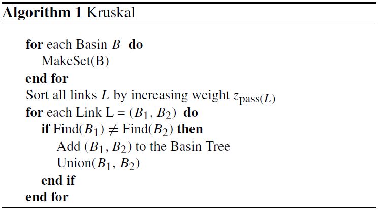
558                                                                        G. Cordonnier et al.: Linear complexity flow routing

the-art algorithms, as reported in the section above. Barnes       tures used for representing flow paths (receivers, donors,
et al. (2014a) propose progressively flooding the topography       and stack), the basin graph, and possibly some additional
from exterior to interior, keeping in a priority queue all the     data structures like those needed by the algorithm of Mareš
parsed nodes except for the ones in depressions, which are         (2002). Some of these data might be required for further pro-
processed using a plain queue. The operations used in this         cessing, e.g., the flow paths in landscape evolution modeling
algorithm can be split in two main categories: one handling        applications. Other data related to the basin graph increase
the nd nodes in depression areas, with nd < n the total num-       the memory consumption, although in practice the number of
ber of nodes, and another one handling the other “regular”         local depressions – and thus the size of the graph – is small
nodes, nr = n − nd , using the priority queue. As a depres-        enough with respect to the size of the grid, resulting in only a
sion encloses at least one node (a local minimum) and zero         small memory overhead compared to the Priority-Flood vari-
or more nodes in the immediate vicinity, the total number of       ants.
nodes in depression areas is always greater than or equal to
the total number of local minima nl , that is, n − nd ≤ n − nl .   5    Conclusions
Therefore, the complexity of Barnes et al. (2014a) Priority-
Flood variant is bounded by k0 +k1 n+k2 (n−nl ) log(n−nl ),        We have presented here a new algorithm for flow path en-
where k0 , k1 , and k2 are constants. Due to the very simple       forcement in topographies with depressions. We have de-
formulation of this algorithm, k1 is very small. The improved      signed this algorithm within the framework of landscape evo-
variants of Priority-Flood proposed by Zhou et al. (2016) and      lution modeling and we have demonstrated through bench-
Wei et al. (2018) further reduce the number of nodes that are      marks that, in this scope, it may greatly improve performance
processed by the priority queue by carefully selecting spill       compared to other state-of-the-art solutions. The potential
candidates among the regular nodes. In those variants, the to-     of this algorithm is, however, not limited to landscape evo-
tal number of nodes processed by the priority queue becomes        lution models. On a broader scope, the basin graph and its
nearly proportional to the number of local minima, inverting       minimum spanning tree are generic structures that other ap-
the formulation of the complexity that is here bounded by          plications may leverage, possibly through derived quantities
k3 + k4 n + k5 nl log nl . Because those variants are more com-    such as the water level of each depression. We propose here
plex, k4 has higher values.                                        optimal methods to compute those structures and quantities.
   We also derive the complexity of our algorithm taking its       Despite the fact that our algorithm is rather complex and re-
stages separately. The first and last stages, i.e., the compu-     quires some work to be properly implemented, it is designed
tation of the basin graph and the update of flow receivers,        in a composable way such that it is easy to reuse one or sev-
are both bounded by k6 + k7 n, with a relatively high value        eral of its components. Adding new features like alternative
for the k6 and k7 constants. The second stage, i.e., the com-      strategies of flow path enforcement within the depressions
putation of the minimum spanning tree, is bounded by ei-           would require only little effort, too.
ther k8 nl log nl when using the Kruskal’s algorithm or k9 nl         While being versatile, this new algorithm does not pro-
when using the algorithm proposed by Mareš (2002), with            vide a universal solution to the problem of flow routing
k8 < k9 . Both expressions above are valid considering that        both within and across closed depressions. Perhaps its main
nl ∼ N values (the number of basins) for N large.                  limitation is the assumption of single- direction flow, i.e.,
   The complexities of the algorithms that we have derived         each node has one unique flow receiver. Adding full support
here are all consistent with the benchmark results shown           for multiple-direction flow (MDF) without losing in perfor-
in Fig. 5a. The difference between the two minimum span-           mance is rather difficult and would require a fair amount of
ning tree algorithms is visible only for a large number of         redesign work at each of the three stages of the algorithm:
local minima, as predicted by their respective asymptotic
complexity, while being unnoticeable for low nl where the              – Basin computation should take into account divergent
other stages of the processing prevail. Similar expressions              flow (basin labels are not unique for grid nodes located
obtained for the complexity of our algorithm vs. the solution            on drainage divides).
based on Wei et al. (2018) are also well illustrated by sub-
parallel curves in the figure. The inverse trend observed for          – It should be theoretically possible to route the outflow
the Barnes et al. (2014a) solution is explained by its complex-          from an inner basin into more than one of its adjacent
ity, where the term (n−nl ) log(n−nl ) tends towards zero as nl          basins (this is currently not possible using a minimum
increases.                                                               spanning tree computed from the basin graph).
   For all the algorithms compared here, the memory con-               – Alternative, MDF-compliant methods should be imple-
sumption grows linearly with the DEM size. Barnes et al.                 mented to update the flow receivers within the depres-
(2014a), Zhou et al. (2016), and Wei et al. (2018) Priority-             sions.
Flood variants only use a supplementary queue to unload
the priority queue, making it very memory-efficient. By con-       Other algorithms like the Priority-Flood do not have that lim-
trast, our algorithm stores more information like the struc-       itation: they act directly on elevation values and do not pre-

Earth Surf. Dynam., 7, 549–562, 2019                                                   www.earth-surf-dynam.net/7/549/2019/
G. Cordonnier et al.: Linear complexity flow routing                                                 559

vent us from applying MDF flow routing methods on the
modified topography.
   Another limitation of this algorithm is its sequential imple-
mentation. Further work is needed to adapt it so that it could
be run on modern, multi-core, and/or GPU-based architec-
tures. Still, many use cases would benefit from the current
implementation. These include processing datasets of mod-
erate size on a single computer or running batches of simu-
lations or analysis pipelines, e.g., in the context of sensitivity
analyses or inferences on model parameters.

www.earth-surf-dynam.net/7/549/2019/                                 Earth Surf. Dynam., 7, 549–562, 2019
560                                                                  G. Cordonnier et al.: Linear complexity flow routing

Appendix A: Algorithms                                        A2   Basin linkage

A1    Basin computation                                       Algorithm 6 creates the graph of basins by linking together
                                                              each pair of adjacent basins. It also finds the passes of low-
Algorithm 5 finds which basin each node of the grid belongs   est elevation between those adjacent basins. Note that the
to by assigning them a label. One unique label is defined     links are undirected, such that Links.contains((b0 , b1 )) ==
(here by an integer) for each basin.                          Links.contains((b1 , b0 )).

Earth Surf. Dynam., 7, 549–562, 2019                                               www.earth-surf-dynam.net/7/549/2019/
G. Cordonnier et al.: Linear complexity flow routing 561
Code availability. The code used for the implementation incision and landscape evolution, Geomorphology, 180, 170–
of the algorithm, examples, and benchmarks presented in 179, https://doi.org/10.1016/j.geomorph.2012.10.008, 2013.
this paper is available here: https://github.com/fastscape-lem/ Campforts, B. and Govers, G.: Keeping the edge: A numeri-
flow-routing-depressions (last access: 13 May 2019; Cordonnier cal method that avoids knickpoint smearing when solving the
et al., 2019). Note that this read-only repository contains a stream power law, J. Geophys. Res.-Earth Surf., 120, 1189–1205,
snapshot version of the fastscapelib library that has been extracted https://doi.org/10.1002/2014JF003376, 2015.
for reproducibility purposes. Further maintenance and new de- Cordonnier, G., Braun, J., Cani, M.-P., Benes, B., Galin, E., Pey-
velopments will happen in the fastscapelib’s main repository: tavie, A., and Guérin, E.: Large scale terrain generation from
https://github.com/fastscape-lem/fastscapelib (last access: 12 tectonic uplift and fluvial erosion, Comput. Graph. Forum, 35,
March 2019; Bovy and Braun, 2019). 165–175, https://doi.org/10.1111/cgf.12820, 2016.
Cordonnier, G., Bovy, B., and Braun, J.: A versatile, linear com-
plexity algorithm for flow routing in topographies with de-
Author contributions. GC designed the algorithm and imple- pressions (code), available at: https://github.com/fastscape-lem/
mented it including the examples/benchmarks presented in this pa- flow-routing-depressions, last access: 13 May 2019.
per; BB also worked on the implementation. GC and BB worked on Jenson, S. and Domingue, J.: Extracting topographic structure from
the redaction of the paper with contributions by JB, and all authors digital elevation data for geographic information system analysis,
contributed to fruitful discussions throughout this study, especially Photogram. Eng. Remote Sens., 54, 1593–1600, 1988.
JB, who provided many test conditions and use cases. Jones, N., Wright, S., and Maidment, D.: Watershed de-
lineation with triangle-based terrain models, J. Hydraul.
Eng., 116, 1232–1251, https://doi.org/10.1061/(ASCE)0733-
Competing interests. The authors declare that they have no con- 9429(1990)116:10(1232), 1990.
flict of interest. Kruskal, J. B.: On the shortest spanning subtree of a graph and
the traveling salesman problem, P. Am. Mathem. Soc., 7, 48–50,
1956.
Lindsay, J. B.: Efficient hybrid breaching-filling sink removal meth-
Acknowledgements. We thank the reviewers for their helpful
ods for flow path enforcement in digital elevation models, Hy-
comments that greatly improved this article.
drol. Process., 30, 846–857, https://doi.org/10.1002/hyp.10648,
2016.
Mareš, M.: Two linear time algorithms for MST on minor closed
Review statement. This paper was edited by Greg Hancock and graph classes, ETHZ, Institute for Mathematical Research, 2002.
reviewed by two anonymous referees. O’Callaghan, J. and Mark, D.: The extraction of drainage networks
from digital elevation data, Comput. Vis. Graph. Image Proc.,
28, 323–344, https://doi.org/10.1016/S0734-189X(84)80011-0,
1984.
References Quinn, P., Beven, K., Chevallier, P., and Planchon, O.: The pre-
diction of hillslope flowpaths for distributed hydrological mod-
Banninger, D.: Technical Note: Water flow routing on ir- eling using digital terrain models, Hydrol. Process., 5, 59–80,
regular meshes, Hydrol. Earth Syst. Sci., 11, 1243–1247, https://doi.org/10.1002/hyp.3360050106, 1991.
https://doi.org/10.5194/hess-11-1243-2007, 2007. Rieger, W.: A phenomenon-based approach to upslope con-
Barnes, R.: Parallel Priority-Flood depression filling for trillion tributing area and depressions in DEMs, Hydrol. Pro-
cell digital elevation models on desktops or clusters, Comput. cess., 12, 857–872, https://doi.org/10.1002/(SICI)1099-
Geosci., 96, 56–68, https://doi.org/10.1016/j.cageo.2016.07.001, 1085(199805)12:63.0.CO;2-B, 1998.
2016. Sambridge, M.: Geophysical inversion with a neighbourhood
Barnes, R.: RichDEM: Terrain Analysis Software, available at: http: algorithm-I. Searching a parameter space, Geophys. J. Int., 138,
//github.com/r-barnes/richdem (last access: 6 November 2018), 479–494, https://doi.org/10.1046/j.1365-246X.1999.00876.x,
2018. 1999.
Barnes, R., Lehman, C., and Mulla, D.: Priority-flood: An Tarboton, D.: A new method for the determination of flow directions
optimal depression-filling and watershed-labeling algorithm and upslope areas in grid digital elevation models, Water Resour.
for digital elevation models, Comput. Geosci., 62, 117–127, Res., 33, 309–319, https://doi.org/10.1029/96WR03137, 1997.
https://doi.org/10.1016/j.cageo.2013.04.024, 2014a. Tucker, G. E. and Hancock, G.: Modelling landscape
Barnes, R., Lehman, C., and Mulla, D.: An efficient as- evolution, Earth Surf. Process. Landf., 35, 28–50,
signment of drainage direction over flat surfaces in raster https://doi.org/10.1002/esp.1952, 2010.
digital elevation models, Comput. Geosci., 62, 128–135, Wei, H., Zhou, G., and Fu, S.: Efficient Priority-Flood depression
https://doi.org/10.1016/j.cageo.2013.01.009, 2014b. filling in raster digital elevation models, Int. J. Dig. Earth, 0, 1–
Boruvka, O.: O jistém problému minimálním, Pràce Moravské 13, https://doi.org/10.1080/17538947.2018.1429503, 2018.
pr̆ìrodovĕdecké spolec̆nosti, 3, 37–58, 1926. Zhou, G., Sun, Z., and Fu, S.: An efficient variant of the
Bovy, B. and Braun, J.: Fastscapelib, available at: https://github. Priority-Flood algorithm for filling depressions in raster
com/fastscape-lem/fastscapelib, last access: 12 March 2019. digital elevation models, Comput. Geosci., 90, 87–96,
Braun, J. and Willett, S. D.: A very efficient O (n), implicit and par- https://doi.org/10.1016/j.cageo.2016.02.021, 2016.
allel method to solve the stream power equation governing fluvial
www.earth-surf-dynam.net/7/549/2019/ Earth Surf. Dynam., 7, 549–562, 2019562 G. Cordonnier et al.: Linear complexity flow routing Zhou, G., Liu, X., Fu, S., and Sun, Z.: Parallel identifi- cation and filling of depressions in raster digital eleva- tion models, Int. J. Geogr. Inform. Sci., 31, 1061–1078, https://doi.org/10.1080/13658816.2016.1262954, 2017. Earth Surf. Dynam., 7, 549–562, 2019 www.earth-surf-dynam.net/7/549/2019/
You can also read