How Did Built Environment Affect Urban Vitality in Urban Waterfronts? A Case Study in Nanjing Reach of Yangtze River - MDPI
←
→
Page content transcription
If your browser does not render page correctly, please read the page content below
International Journal of
               Geo-Information

Article
How Did Built Environment Affect Urban Vitality in Urban
Waterfronts? A Case Study in Nanjing Reach of Yangtze River
Zhengxi Fan             , Jin Duan *, Menglin Luo, Huanran Zhan, Mengru Liu and Wangchongyu Peng

                                          Department of Urban Planning, School of Architecture, Southeast University, Nanjing 210096, China;
                                          fanzx0058@seu.edu.cn (Z.F.); luoml@seu.edu.cn (M.L.); zhanhr@seu.edu.cn (H.Z.); liumr@seu.edu.cn (M.L.);
                                          pengwcy@seu.edu.cn (W.P.)
                                          * Correspondence: seduanjin@seu.edu.cn

                                          Abstract: The potential of urban waterfronts as vibrant urban spaces has become a focus of urban
                                          studies in recent years. However, few studies have examined the relationships between urban vitality
                                          and built environment characteristics in urban waterfronts. This study takes advantage of emerging
                                          urban big data and adopts hourly Baidu heat map (BHM) data as a proxy for portraying urban vitality
                                          along the Yangtze River in Nanjing. The impact of built environment on urban vitality in urban
                                          waterfronts is revealed with the ordinary least squares (OLS) and geographically weighted regression
                                          (GWR) models. The results show that (1) the distribution of urban vitality in urban waterfronts
                                          shows similar agglomeration characteristics on weekdays and weekends, and the identified vibrant
                                          cores tend to be the important city and town centers; (2) the building density has the strongest

                                   positive associations with urban vitality in urban waterfronts, while the normalized difference
                                          vegetation index (NDVI) is negative; (3) the effects of the built environment on urban vitality in
Citation: Fan, Z.; Duan, J.; Luo, M.;
Zhan, H.; Liu, M.; Peng, W. How Did
                                          urban waterfronts have significant spatial variations. Our findings can provide meaningful guidance
Built Environment Affect Urban            and implications for vitality-oriented urban waterfronts planning and redevelopment.
Vitality in Urban Waterfronts? A Case
Study in Nanjing Reach of Yangtze         Keywords: urban waterfronts; urban vitality; built environment; big data; geographically weighted
River. ISPRS Int. J. Geo-Inf. 2021, 10,   regression; Yangtze River
611. https://doi.org/10.3390/
ijgi10090611

Academic Editors: Wolfgang Kainz,         1. Introduction
Christos Chalkias, Vassilis Pappas
                                                Urban waterfronts, as the important part of a town or city adjoining water area (i.e.,
and Andreas Tsatsaris
                                          river, lake, sea and ocean, and harbor), have a unique spatial interface and attractive
                                          waterscape [1–4]. Moreover, urban waterfronts also have obvious advantages in terms of
Received: 29 July 2021
Accepted: 13 September 2021
                                          economic development, ecological environment, social interaction, and cultural heritage
Published: 15 September 2021
                                          [5–8]. The redevelopment of urban waterfronts, which has become a well-established
                                          global trend, provides urban waterfronts with new functions (e.g., leisure, recreation, retail,
Publisher’s Note: MDPI stays neutral
                                          and tourism) to satisfy both economic and social needs [9–13]. In recent decades, a growing
with regard to jurisdictional claims in
                                          body of studies has focused on the redevelopment of urban waterfronts as an important
published maps and institutional affil-   way for cities to improve their vitality, attraction, and international competitiveness [14–16].
iations.                                  In China, the development of urban waterfronts is now facing new opportunities for
                                          transformation and redevelopment [17–19]. Therefore, assessing urban vitality in urban
                                          waterfronts and deciphering its influencing mechanisms are crucially important for urban
                                          waterfronts planning and design.
Copyright: © 2021 by the authors.
                                                The concept of urban vitality is brought into view by Jacobs [20] when it was noted
Licensee MDPI, Basel, Switzerland.
                                          that the presence of more active streets could encourage more people to engage in various
This article is an open access article
                                          activities, whether commercial or residential. Jacobs maintained that vibrant urban space
distributed under the terms and           was positive to create a diverse city life. Lynch [21] later defined urban vitality as to
conditions of the Creative Commons        what extent vital functions and biological requirements of individual are buttressed by
Attribution (CC BY) license (https://     the capacity of the environment. Maas [22] described urban vitality as a representation of
creativecommons.org/licenses/by/          spatial quality involving the continuous presence of people, activities and opportunities, as
4.0/).                                    well as the physical environment in which these activities occur. Montgomery [23] claimed

ISPRS Int. J. Geo-Inf. 2021, 10, 611. https://doi.org/10.3390/ijgi10090611                                      https://www.mdpi.com/journal/ijgi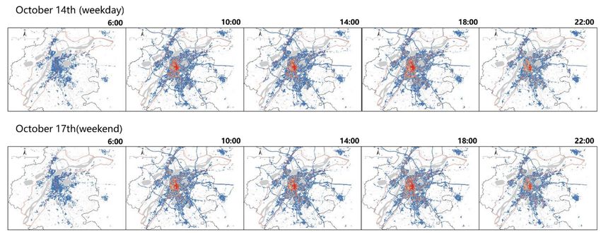
ISPRS Int. J. Geo-Inf. 2021, 10, 611                                                                                            2 of 18

                                       that the characteristics of successful urban places tend to have a more vibrant public realm
                                       breeding rich human activities. While there is no consensus on the definition of urban
                                       vitality, human interactions as well as activities have commonly been the focus of urban
                                       vitality research.
                                             In the era of big data, the availability of massive crowdsourced data has become
                                       a prominent part of characterizing urban vitality in geography and urban studies [24].
                                       Generally, current research of urban vitality can be categorized into two streams: measuring
                                       urban vitality and examining its determinants. The first research stream applies various
                                       crowdsourced data to assess the spatiotemporal characteristics of urban vitality. The
                                       mobile phone data, social media data, GPS tracking data, as well as Baidu heat map
                                       (BHM) data serve as the most dominant proxies of urban vitality by reason that these
                                       data provide detailed information regarding people’s behavioral characteristics [25–29].
                                       The second research stream delves into the relationship between urban vitality and its
                                       determinants. Scholars claimed that built environment characteristics, such as building
                                       density, development intensity, and transportation network, have significant effects on
                                       urban vitality [30–34]. These studies have enriched the literature of urban vitality and
                                       provided meaningful insights for creating vibrant urban space. For example, well-designed
                                       public spaces and small street blocks provide opportunities for more diverse human
                                       activities and interactions, and thus foster livable streets and vibrant neighborhoods [35–37].
                                       However, most previous studies ignore the spatiotemporal analysis of urban vitality in
                                       specific areas, especially for urban waterfronts. Therefore, it is necessary to apply reliable
                                       crowdsourced data to effectively assess urban vitality in urban waterfronts.
                                             In this paper, the BHM data collected in Nanjing is adopted to investigate the spa-
                                       tiotemporal analysis of urban vitality in urban waterfronts. Besides, both ordinary least
                                       squares (OLS) and geographically weighted regression (GWR) models are used to quantify
                                       the associations between urban vitality and built environment characteristics in urban
                                       waterfronts. This study is intended to (1) explore the spatiotemporal characteristics of
                                       urban vitality in urban waterfronts through the analysis of BHM data; (2) examine how
                                       built environment characteristics correlates with urban vitality in urban waterfronts; and
                                       (3) afford useful insights and references as to fostering urban vitality in urban waterfronts.

                                       2. Literature Review
                                       2.1. The Measurements of Urban Vitality
                                            Urban vitality, as a vital element for achieving a higher quality of human life, de-
                                       scribes the attractiveness, diversity, and competitiveness of public spaces [25,38]. However,
                                       how to accurately measure urban vitality remains a challenging issue. Traditional data
                                       collection methods, such as field survey and on-site observation, provide detailed human
                                       activities information that includes gender, age, characteristics, and activities and behavior
                                       of users [39,40]. Such methods, however, are usually costly and time-consuming, and thus
                                       may not be suitable for investigating urban vitality at a large scale [41].
                                            Fortunately, in recent years, the rise of crowdsourced data sources, notably data de-
                                       rived from mobile phones as well as social media, offer massive opportunities for observing
                                       various human activities and interactions [24]. For example, Nadai et al. [42] proposed a
                                       method to measure urban vitality with mobile phone records and examined the association
                                       between urban vitality and diversity in the Italian context. Yue et al. [26] quantified neigh-
                                       borhood vitality based on mobile phone data and investigated the association between the
                                       point of interest (POI)-based mixed use and neighborhood vitality. Wu et al. [25] suggested
                                       that social media check-in data can be used as a proxy for characterizing spatiotemporal
                                       patterns of urban vitality in Shenzhen. Recently, BHM data, as a kind of crowdsourced
                                       data regarding human activity, provide a new angle to portray population distribution
                                       and urban dynamics [43,44]. Numerous novel studies have tapped into the BHM data as a
                                       crucial tool in the research of green spaces and parks [43,45,46], urban population aggre-
                                       gation characteristics [47,48], and urban structure and land use [49]. In contrast to social
                                       media data and other traditional datasets, BHM data can provide real-time analysis for the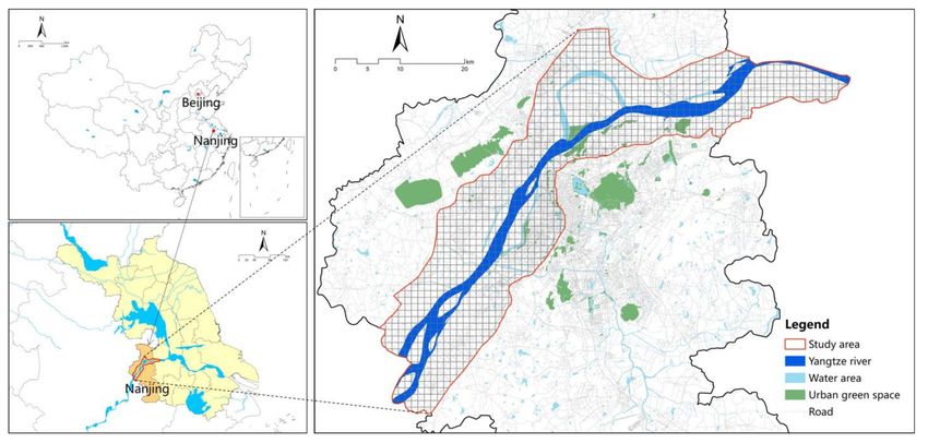
ISPRS Int. J. Geo-Inf. 2021, 10, 611                                                                                           3 of 18

                                       dynamics of human activities on daily or hourly intervals [43]. However, comprehensive
                                       studies using BHM data to characterize urban vitality are rare, thus this study attempts
                                       to adopt the BHM data as the proxy for describing the spatiotemporal characteristics of
                                       urban vitality in urban waterfronts.

                                       2.2. The Relationship between Built Environment and Urban Vitality
                                             According to classical theories in urban planning and design [20,23,50], the built
                                       environment proves to produce significant effects on the creation of urban vitality in urban
                                       spaces. Many existing attempts to link urban analytics and design have been less well-
                                       received by urban planners and designers [32], while Salingaros [51] and Alexander [52]
                                       have called for new analytical processes, which are derived from principles in urban
                                       structure and complexity, are applied in urban design. More recently, substantial efforts
                                       have been devoted to examining the relationship between built environment and urban
                                       vitality integrated with quantitative analysis [27,32,33,41]. For example, Jacobs-Crisioni
                                       et al. [53] investigated the impact of dense and mixed land use on urban activity intensity
                                       in Amsterdam, and verified that higher densities and mixed land use contribute to higher
                                       urban vitality. Sung et al. [54] attempted to apply Jacobs’s urban design theory to study the
                                       urban vitality of Seoul, and the empirical findings point to the significant role of mixed
                                       use, small-scale blocks, as well as density in improving the urban vitality. Conducted
                                       a study for five megacities in China, Xia et al. [55] found a remarkable positive spatial
                                       autocorrelation that connects urban land use intensity with urban vitality based on a local
                                       indicator of spatial association (LISA) method. Mouratidis and Poortinga [37] provided
                                       evidence that neighborhood density and land use mix are positively associated with urban
                                       vitality, whereas green space is found to be associated with lower urban vitality.
                                             Furthermore, the traditional global regression model (e.g., OLS regression model) has
                                       been verified as an effective method in unearthing the impact of various built environment
                                       characteristics on urban vitality [27,31,41]. However, the global regression model may not
                                       be able to adequately exhibit the spatial nonstationarity and actual phenomena, as the
                                       obtained global relationships are constant within the entire study area and can only reflect
                                       the average conditions [56,57]. In this context, the geographically weighted regression
                                       (GWR) model, which overcomes the limitations of the global regression model (i.e., OLS)
                                       and can effectively solve the problem of spatial nonstationarity, was introduced to explore
                                       the geographical varying relationship by direct simulation of local nonstationary data
                                       [58–60]. Although GWR has been widely applied in many fields of applied geography
                                       [58,61,62], the efforts are still insufficient to uncover the local correlations between built
                                       environment characteristics and urban vitality in urban waterfronts.
                                             From the above review, it is apparent that urban vitality has close associations with
                                       the built environment variables. Nevertheless, researches that put their focus on the impact
                                       of built environment characteristics on urban vitality in urban waterfronts are still limited.
                                       Furthermore, few studies have applied the GWR model to investigate the spatial variations
                                       in the influence of built environment on urban vitality. Therefore, this article serves as an
                                       attempt to extend and expand the previous research by quantifying the associations that
                                       connect built environment characteristics and urban vitality in urban waterfronts based on
                                       the BHM data and the application of OLS and GWR models.

                                       3. Data and Methods
                                       3.1. Study Area
                                            Nanjing, a historical city located in the Yangtze River Delta region of eastern China, is
                                       the capital of Jiangsu Province. The Yangtze River runs through the city and divides it into
                                       two regions. The development strategy of Nanjing city centers on creating a humanistic,
                                       green and innovative modern city that enjoys international reputation and global influ-
                                       ence [63]. For the development of Nanjing city, urban waterfronts along the Yangtze River
                                       have a great development potential, the important urban landscape and tourist resource,
                                       as well as the symbol of geography, history and culture. Combining with neighborhoods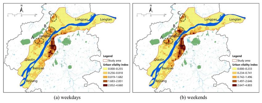
ISPRS Int. J. Geo-Inf. 2021, 10, 611                                                                                          4 of 18

                                       and road networks along the Yangtze River, this study focused on the urban waterfronts
                                       with a range of 3–6 km from the shoreline along the Yangtze River in Nanjing (Figure 1).

                                  Figure 1. Study area: urban waterfronts along the Yangtze River in Nanjing.

                                            The analytic unit for studying urban vitality is important [26]. Based on the previous
                                       research that focused on the spatial analysis of urban vitality with big data [25,33], this
                                       study applied a grid-based method (spatial resolution 1 km * 1 km) as the neighborhood-
                                       scale unit to measure spatiotemporal urban vitality in urban waterfronts, and then to
                                       explore how built environment variables is related to urban vitality. As shown in Figure 1,
                                       the study area can be divided into 1239 spatial units.

                                       3.2. Data
                                       3.2.1. BHM Data
                                             BHM, as a common type of crowdsourced data in China, provides a powerful tool
                                       to describe the real-time distribution, density, and dynamics of population. This crowd-
                                       sourced data gathers the geolocated locations provided by the mobile phone users who
                                       use application products provided by Baidu (e.g., Baidu search, Baidu map, and Baidu
                                       cloud, etc.), and then displays the relative population distinguished by colors, where red
                                       represents high density, and blue represents low density (Figure 2). Recent studies have
                                       verified that BHM data could be used as a reasonable proxy for measuring the dynamics of
                                       human activities in different areas [29,43]. In this study, therefore, the BHM data at hourly
                                       intervals from 6:00 to 22:00 across the Nanjing city were collected on a weekday (October
                                       14th in 2020, Wednesday) and a weekend (October 17th in 2020, Saturday) (Figure 2). In
                                       total, 34 BHMs (spatial resolution 3.5 m * 3.5 m) were adopted for analysis.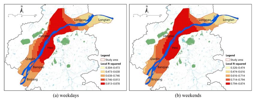
ISPRS Int. J. Geo-Inf. 2021, 10, 611                                                                                            5 of 18

                        Figure 2. The sample data of BHM data collected on October 14th and October 17th in 2020.

                                       3.2.2. Other Complementary Data
                                            In this research, multi-source data were employed to quantify built environment
                                       characteristics, including point of interest (POI), building footprints, bus and subway
                                       stations, polygon of the Yangtze River, and the normalized difference vegetation index
                                       (NDVI) data. POI datasets were collected from Baidu map (available from https://map.
                                       baidu.com/ (accessed on 25 August 2021)), which provides free API interfaces and detailed
                                       location information on geographic entities, such as commercial facilities, traffic facilities,
                                       and green spaces and squares. These data have substantially assisted many earlier related
                                       studies to reflect land use [25,27]. In our study, therefore, as many as 264,001 POIs were
                                       adopted to measure functional density and mixed use. The detailed building footprint data
                                       was also acquired from Baidu map (available from https://map.baidu.com/), and served
                                       the effort to evaluate the building density and floor area ratio. The information as to transit
                                       stations/stops were derived from Nanjing public transportation website (available from
                                       http://nanjing.gongjiao.com/ (accessed on 25 August 2021)). Such data, which provides
                                       useful traffic information, were utilized to measure the distance to public transport stations.
                                       Polygon data of the Yangtze River, which was derived from the Nanjing Master Planning
                                       (2011–2020) [63], was used to measure the distance to shoreline. The NDVI data (spatial
                                       resolution 30 m ∗ 30 m) was calculated based on the Landsat 8 OLI image, which was
                                       downloaded from the Geospatial Data Cloud (available from http://www.gscloud.cn/
                                       (accessed on 25 August 2021)). This vegetation data was used to measure the degree of
                                       vegetation coverage for urban waterfronts.

                                       3.3. Methods
                                       3.3.1. Evaluating Urban Vitality in Urban Waterfronts
                                             The BHM data, as an important population-oriented visualization product, could
                                       directly indicate real-time population density as distinguished by colors on the map [45,64].
                                       This data ranges from 0 to 7 and the larger value means more human activities. Fan
                                       et al. [43] proposed a method to assess the vitality of urban parks through BHM data. This
                                       study adopted the BHM data-based method for measuring urban vitality and calculated
                                       the average urban vitality value of each spatial unit. The calculation was performed using
                                       a so-called “Zonal Statistics” in ArcGIS 10.5, which referenced the BHM data-based method
                                       described by Fan et al. [43]. The average urban vitality value can be quantified as follows:

                                                                                      ∑in=1 Ai
                                                                               Qi =                                                (1)
                                                                                       n ∗ Si
ISPRS Int. J. Geo-Inf. 2021, 10, 611 6 of 18
where Qi is the average urban vitality of spatial unit i of per day, Ai is the urban vitality
of spatial unit i at a given time, Si is the area of spatial unit i, n = 6:00, 7:00, 8:00, . . . 22:00
(17 time slots).
3.3.2. Associated Built Environment Variables
Good built environment features tend to promote the development of vibrant streets,
neighborhoods, and of course, urban waterfronts [23,31,33]. Previous studies have sug-
gested that many built environment characteristics are associated with urban vitality,
include building density, road intersections, functional density, mixed land use, greenspace,
and accessibility [26,27,32,33,37,65]. Based on previous studies and data availability, we
established built environment variables from four major dimensions, namely density, di-
versity, accessibility, and vegetation. The density dimension has three variables, namely the
building density, floor area ratio, road intersections, and functional density. The diversity
dimension is mainly measured by mixed use. The accessibility dimension including two
variables, namely the distance to public transport stations and the distance to shoreline.
The vegetation dimension is mainly measured by the NDVI. The detailed quantification
variables are listed in Table 1.
Table 1. Description of built environment variables.
Dimensions Variables Abbr. Descriptions Data Source
Building
BD The building density of each square kilometer grid map.baidu.com (2020)
density
Density Floor area ratio FAR The floor area ratio of each square kilometer grid map.baidu.com (2020)
Road The number of road intersections of each square
RI Open Street Map (2020)
intersections kilometer grid
Functional
FD The number of POI of each square kilometer grid map.baidu.com (2020)
density
The Shannon entropy is used to calculate the mixed
n
use [27,41], D = −∑ pi ln( pi ), where D is mixed use
1
index, pi is the proportions of each of the POI types
Diversity Mixed use MU map.baidu.com (2020)
(residential POI, commercial POI, traffic POI, office
POI, science, education and health POI, and green
space and square POI), and n is the number of the
POI types, in this case n = 6.
Distance to
The distance to the nearest bus or subway stations of nanjing.gongjiao.com
public transport DPTS
Accessibility each square kilometer grid (2020)
stations
Distance to The distance to the nearest shoreline of each square Nanjing master
DS
shoreline kilometer grid planning (2011–2020)
Normalized
The average value of NDVI of each square kilometer Landsat 8 OLI, spatial
difference N IR− Red
Vegetation NDVI grid, NDV I = N IR+ Red , where N IR denotes
resolution 30 m × 30 m
vegetation
near-infrared band, and Red is the red band. (2020)
index
3.3.3. Global and Local Regression Models
Initially, this article explored the relations that connect urban vitality and built envi-
ronment in urban waterfronts from a global perspective. The global regression model is
conducted by the OLS regression model, which serves as a commonplace and effective
statistical model for research concerning urban vitality [33,66]. The OLS regression is
expressed as thus:
m
y = β0 + ∑ β j xj + ε (2)
j =1
where y stands for the dependent variable, x j for the jth built environment indicators, β j
for the corresponding estimated coefficient, ε and for the residual.ISPRS Int. J. Geo-Inf. 2021, 10, 611 7 of 18
Second, this study investigated the spatial heterogeneity in the effect of built en-
vironment on urban vitality in urban waterfronts from a local perspective. The local
regression model is conducted by the GWR model, which is a location-dependent method
to characterize the spatial nonstationarity by fitting a regression model at each local ob-
servation, weighting nearby observations around each subject point based on a distance
decay function [67]. The GWR model is formulated as follows:
m
yi = β 0 (ui , vi ) + ∑ β j (ui , vi ) x ji + ε i (3)
i =1
where i represents the spatial unit i, yi denotes the value of urban vitality of the spatial
unit i, x ji is the jth built environment indicators of the spatial unit i, m stands for the
total number of spatial units, ε i denotes the random error term of the spatial unit i, (ui , vi )
signifies the location of spatial unit i, β 0 (ui , vi ) stands for the intercept at the location i, and
β j (ui , vi ) represents the local estimated coefficient of the built environment variable x ji .
For the geographical weighting function, a fixed Gaussian distance decay function [56],
which assumes that things in closer proximity give rise to more robust influence, is adopted
in our study. The bandwidth defines the scope of the spatial weighting function and in
the meantime bears on the degree of the local regression model’s calibration [67]. The
weighting function along with the best bandwidth size in the model adopted is determined
through the corrected Akaike information criterion (AICc), which demonstrates the extent
to which the model is consistent with actual phenomena, and the numbers of degrees of
freedom in the varied models are considered too [68].
4. Results
4.1. Characteristics of Urban Vitality in Urban Waterfronts
According to the BHM data, urban vitality values were classified into as many as
five grades according to natural breaks in ArcGIS 10.5. In general, Figure 3 illustrates that
urban vitality in urban waterfronts displays similar spatial distributions on weekdays and
weekends, although local differences can be observed. Specifically, as shown in Table 2,
the maximum and mean of urban vitality in urban waterfronts on weekends (maximum of
4.803 and mean of 0.382) are slightly higher than that on weekdays (maximum of 4.660 and
mean of 0.380).
Figure 3. Spatial characteristics of urban vitality index in urban waterfronts: (a) urban vitality on weekdays; (b) urban
vitality on weekends.ISPRS Int. J. Geo-Inf. 2021, 10, 611 8 of 18
Table 2. The statistical characteristics of urban vitality index in urban waterfronts on weekdays
and weekends.
Maximum Minimum Mean Median SD
weekdays 4.660 0.000 0.380 0.041 0.715
weekends 4.803 0.000 0.382 0.029 0.737
In addition, the distribution of urban vitality in urban waterfronts shows obvious
agglomeration characteristics on both weekdays and weekends. Figure 3 demonstrates
that the identified vibrant core in urban waterfronts located in the southern Yangtze River
regions are the urban central areas (Hexi), whereas the northern regions are mainly town
centers of Nanjing, including Zhujiang (A in Figure 3), Qiaobei (B in Figure 3), and Dachang
(C in Figure 3). These identified vibrant cores are basically consistent with the urban growth
of Nanjing.
4.2. OLS Regression Analysis and Global Relationships
The OLS regression model was deployed to examine the global relationship between
urban vitality on weekdays and weekends and built environment characteristics in urban
waterfronts. As the regression results are reported in Tables 3 and 4, BD, FAR, RI, FD, MU,
DPTS, DS, and NDVI are significantly associated with urban vitality on weekdays and
weekends in urban waterfronts along the Yangtze River in Nanjing. All of these variables
are significant at the 0.05 confidence level. The adjusted R square is 0.850 for weekdays
and 0.843 for weekends, thus verifying that the independent variables determined are
able to explain 85.0% and 84.3% of the urban vitality on weekdays and weekends in
urban waterfronts. In addition, this study examined the variance inflation factor (VIF)
values of each built environment variable, which are all far less than 10, indicating that no
multi-collinearity exists between the independent variables.
Table 3. Regression results of urban vitality by OLS model on weekdays.
Variable Coefficient t-Statistic Std. VIF
BD 1.021 5.315 ** 0.192 4.874
FAR 0.182 5.309 * 0.034 5.784
RI 0.020 7.20 ** 0.003 1.983
FD 0.002 29.812 ** 0.000 3.085
MU 0.065 5.106 ** 0.012 1.813
DPTS −0.014 −1.484 ** 0.009 1.447
DS 0.032 6.493 ** 0.005 1.362
NDVI −0.290 −3.717 ** 0.078 1.383
AICs = 346.960
Adjusted R2 = 0.850
* significant at the 0.05 level, ** significant at the 0.001 level.
Table 4. Regression results of urban vitality by OLS model on weekends.
Variable Coefficients t-Statistic Std. VIF
BD 0.690 3.407 ** 0.203 4.874
FAR 0.291 8.069 ** 0.036 5.784
RI 0.015 5.143 ** 0.003 1.983
FD 0.002 28.709 ** 0.000 3.085
MU 0.053 3.993 ** 0.013 1.813
DPTS −0.016 −1.681 ** 0.010 1.447
DS 0.033 6.309 ** 0.005 1.362
NDVI −0.269 −3.276 ** 0.082 1.383
AICs = 479.678
Adjusted R2 = 0.843
** significant at the 0.001 level.ISPRS Int. J. Geo-Inf. 2021, 10, 611 9 of 18
Moreover, Tables 3 and 4 show that the BD, FAR, RI, FD, MU, and DS have positive
associations with the urban vitality in urban waterfronts. Among all built environment
variables, the BD (1.021 for weekdays and 0.690 for weekends) has the strongest positive
associations with urban vitality in urban waterfronts, followed by another density variable,
FAR (0.182 for weekdays and 0.291 for weekends), demonstrating that high-density is
significantly correlated with sustained urban vitality. Besides, our results show that the MU
(0.065 for weekdays and 0.053 for weekends) has a positive correlation with urban vitality
in urban waterfronts, which overlaps with Jacobs’s view that a diversity of urban functions
motivate to spend more time around urban spaces and undertake varied activities. The DS
(0.032 for weekdays and 0.033 for weekends) has positive associations with urban vitality
in urban waterfronts, demonstrating that the more proximity to the shoreline, the lower
urban vitality. As shown in Tables 3 and 4, the DPTS (−0.014 for weekdays and −0.016
for weekends) is found to have a negative association with urban vitality, thus indicating
that convenient public transport can generate more urban vitality in urban waterfronts.
Notably, the NDVI (−0.290 for weekdays and −0.269 for weekends) has a significant
negative association with urban vitality in urban waterfronts.
4.3. GWR Analysis and Spatial Variations
A further examination with GWR models was conducted to provide an insightful
understanding of the local correlations between urban vitality and built environment in
urban waterfronts. As shown in Tables 5 and 6, the adjusted R-squared values of GWR
models (0.880 for weekdays and 0.871 for weekends) have increased in contrast with
those derived from OLS regression models (0.850 for weekdays and 0.843 for weekends).
Furthermore, the AICs values of GWR models (111.032 for weekdays and 269.201 for
weekends) are remarkably lower than those of OLS regression models (346.960 for week-
days and 479.678 for weekends). The improvement of adjusted R-squared values and the
significant decrease in AICs values indicate that the GWR model has a better capability to
interpret the correlations between built environment characteristics and urban vitality in
urban waterfronts.
Table 5. Regression results of urban vitality by GWR model on weekdays.
Lower Upper
Variable Mean Std. Min Median Max
Quartile Quartile
BD 0.734 1.564 −1.676 −0.065 0.761 1.104 13.239
FAR 0.322 0.308 −0.609 0.194 0.539 1.084 2.646
RI 0.016 0.009 −0.008 0.011 0.014 0.023 0.037
FD 0.002 0.001 −0.000 0.001 0.002 0.002 0.004
MU 0.049 0.042 −0.041 0.021 0.035 0.079 0.183
DPTS −0.040 0.040 −0.195 −0.059 −0.025 −0.010 −0.001
DS 0.037 0.035 −0.001 0.016 0.020 0.050 0.137
NDVI −0.223 0.149 −0.894 −0.281 −0.188 −0.114 −0.006
AICs = 111.032
Adjusted R2 = 0.880ISPRS Int. J. Geo-Inf. 2021, 10, 611 10 of 18
Table 6. Regression results of urban vitality by GWR model on weekends.
Lower Upper
Variable Mean Std. Min Median Max
Quartile Quartile
BD 0.392 1.516 −2.913 −0.506 0.398 0.925 11.171
FAR 0.377 0.268 −0.445 0.264 0.355 0.409 2.266
RI 0.012 0.010 −0.014 0.006 0.009 0.018 0.035
FD 0.002 0.001 0.000 0.002 0.002 0.002 0.004
MU 0.030 0.035 −0.059 0.017 0.030 0.065 0.130
DPTS −0.024 0.047 −0.214 −0.077 −0.024 −0.009 −0.000
DS 0.038 0.034 −0.001 0.017 0.026 0.048 0.141
NDVI −0.211 0.132 −0.732 −0.269 −0.177 −0.112 −0.000
AICs = 269.201
Adjusted R2 = 0.871
Figure 4 demonstrates that under the GWR models, the spatial characteristics of
local R-squared values are similar on weekdays and weekends. The local R-squared
values exhibit notable spatial variations, demonstrating that the explanatory capacity of
the GWR models is different for the spatial location of urban waterfronts. It is obvious
that the central regions of urban waterfronts (Hexi and Jiangbei) have a relatively higher
explanatory capacity with the GWR models. In addition, it is detected that the spatial
characteristics of the local R-squared value display a decay tendency from central regions
to peripheral areas.
Figure 4. Spatial characteristics of local R-squared values with the GWR model: (a) local R-squared values on weekdays;
(b) local R-squared values on weekends.
Figures 5 and 6 make it clear that with respect to the spatial variations of local esti-
mated coefficients of all the built environment variables on weekdays and weekends, the
deeper color represents larger coefficients. For variables positively related, darker colors
stand for a stronger positive effect, while for variables negatively related, such as DPTS
and NDVI, paler colors denote a stronger negative effect.ISPRS Int. J. Geo-Inf. 2021, 10, 611 11 of 18
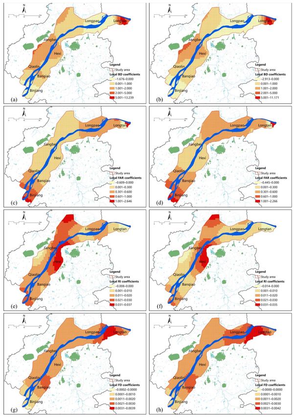
Figure 5. Spatial characteristics of estimated coefficients of built environment variables with GWR: (a) local BD coefficients
on weekdays; (b) local BD coefficients on weekends; (c) local FAR coefficients on weekdays; (d) local FAR coefficients on
weekends; (e) local RI coefficients on weekdays; (f) local RI coefficients on weekends; (g) local FD coefficients on weekdays;
(h) local FD coefficients on weekends.ISPRS Int. J. Geo-Inf. 2021, 10, 611 12 of 18
Figure 6. Continued: (a) local MU coefficients on weekdays; (b) local MU coefficients on weekends; (c) local DPTS
coefficients on weekdays; (d) local DPTS coefficients on weekends; (e) local DS coefficients on weekdays; (f) local DS
coefficients on weekends; (g) local NDVI coefficients on weekdays; (h) local NDVI coefficients on weekends.
As shown in Figure 5, the BD, FAR, RI, and FD were found to have positive impacts
on the urban vitality in most urban waterfronts on weekdays and weekends. Figure 5a,bISPRS Int. J. Geo-Inf. 2021, 10, 611 13 of 18
illustrate that BD had a more significant positive impact on the urban vitality in the central
and western regions of urban waterfronts (Hexi, Jiangbei, and Longtan). Figure 5c,d
demonstrate that FAR presents a greater positive driving on the urban vitality in the
eastern and western regions of urban waterfronts (Longtan and Binjiang). This influence
dwindled by degrees from the outer to the center. Figure 5e,f show that RI had a slight
positive driving on the urban vitality in the various urban waterfronts. Figure 5g,h depict
that FD had a slight positive driving on the urban vitality in the western regions of urban
waterfronts (Longtan, and Longpao), whereas a slight negative driving in the eastern
regions of urban waterfronts (Binjiang).
As shown in Figure 6, the MU and DS were found to have positive impacts on the
urban vitality in most urban waterfronts on weekdays and weekends, while DPTS and
NDVI show significant negative influences on the urban vitality. For MU, a remarkable
positive effect took place in the central regions of urban waterfronts (Hexi and Jiangbei),
whereas a negative effect was detected in the northern area (Figure 6a,b). For DS, the spatial
characteristics of the correlation coefficients were higher in the central regions of urban
waterfronts (Hexi and Jiangbei), and the impacts gradually decreased from the core area
to the suburbs (Figure 6e,f). Figure 6c,d demonstrate that DPTS has a significant negative
effect in the central regions of urban waterfronts (Hexi and Jiangbei). With regard to NDVI,
a strong negative effect can be observed in various regions of urban waterfronts, and the
central regions of urban waterfronts located in the southern Yangtze River regions (Hexi)
have the strongest negative effect (Figure 6g,h).
In a word, the variables in relation to built environment characteristics and urban
vitality present significant spatial variation within the whole area studied, demonstrating
the spatial nonstationary relations between these variables and urban vitality in urban
waterfronts. The OLS model provides the global associations that connect built environ-
ment characteristics and urban vitality in urban waterfronts, and the GWR model further
discovers some distinctive differences in various regions by taking account of spatial
autocorrelation and spatial heterogeneity.
5. Discussion
5.1. Towards Establishing a BHM Data-Based Method for Assessing Urban Vitality in
Urban Waterfronts
Emerging crowdsourced data enable urban planners and policymakers to assess urban
vitality with less expense but more efficiency [24]. In particular, real-time crowdsourced
data provides a dynamic perspective for urban space. However, how to develop an effec-
tive and accurate method to assess spatiotemporal urban vitality remains a challenging
issue. Therefore, this study aims to propose a BHM data-based approach to assess spa-
tiotemporal urban vitality in urban waterfronts, which is a response to the increasing
interest in adopting emerging crowdsourced data and new analytical methods into urban
vitality studies [25,32]. The results suggest that the distribution of urban vitality in urban
waterfronts shows similar agglomeration characteristics on weekdays and weekends. Fur-
thermore, the identified vibrant cores based on the BHM data tended to be the important
city and town centers, which is largely consistent with the urban growth of Nanjing city.
It is also supported by an earlier study pointing out that the identified vibrant cores are
mainly town centers in Shanghai city [33]. This study suggests that the BHM data-based
method can be extended to other rapidly urbanizing areas.
5.2. The Influencing of Built Environment Characteristics on Urban Vitality in Urban Waterfronts
Understanding the relationship between built environment characteristics and urban
vitality could provide significant implications for cultivating more vibrant urban spaces
and enhancing the urban quality of life. In this study, OLS and GWR models are employed
to quantify the association between urban vitality and built environment characteristics in
urban waterfronts. The OLS regression results indicate that the BD (1.021 for weekdays
and 0.690 for weekends), FAR (0.182 for weekdays and 0.291 for weekends), and MUISPRS Int. J. Geo-Inf. 2021, 10, 611 14 of 18
(0.065 for weekdays and 0.053 for weekends) have a remarkable influence on urban vitality
in urban waterfronts. This finding can further support the importance of density and
diversity in urban spaces, which was empirically evidenced by recent studies [31,32].
Dovey and Pafka [69] also provided convincing evidence that density concentrates more
people and places within walkable distances and diversity produces a greater range of
walkable destinations. Besides, the results show that the NDVI (−0.290 for weekdays
and −0.269 for weekends) has a significant negative association with urban vitality in
urban waterfronts. This suggests that more vegetation coverage may restrain the sense of
liveliness. A study by Mouratidis and Poortinga [37] in Oslo metropolitan area, also found
that a negative relationship exists between green space and urban vitality. In some sense,
the low urban vitality can be said to partly account for the calming and restorative effects
of green spaces [70].
The GWR model also proves effective to analyze the local associations between vari-
ables under the category of built environment and urban vitality in urban waterfronts. As
shown in Figures 5 and 6, the correlations of the built environment variables with urban
vitality exhibit considerable spatial variations within the whole area studied. It reflects the
impact of built environment variables on urban vitality has apparent spatial heterogeneity.
Specifically, taking variables such as BD and MU as examples, more significant positive
impacts on urban vitality in urban waterfronts were found in the central regions (Hexi and
Jiangbei), whereas negative impacts were found in the peripheral area. For DPTS, a strong
negative effect can be observed in the central regions (Hexi and Jiangbei), demonstrating
that these regions have more convenient public transport, and then higher urban vitality.
A study by Liu et al. [71] also showed that traffic access and land use mix have strong
positive correlations with urban vitality in the central area rather than peripheral area.
Besides, our findings suggest that the DS has positive associations with urban vitality in
urban waterfronts, especially in the central regions (Hexi and Jiangbei), demonstrating
that the more proximity to the shoreline, the lower urban vitality. Similarly, a study by
Liu et al. [18] in Shanghai city, showed that traffic accessibility has a negative effect on
the urban vitality in urban waterfronts. This could be attributable to that several urban
waterfronts near the central regions in our study are characterize by less connectivity to the
shoreline and monotonous landscape. Therefore, it is important to realize that the openness
of shoreline and diversity landscape of urban waterfronts will enhance the vitality of urban
waterfronts.
5.3. Limitations and Future Studies
This study also has several limitations. First, even though the BHM data can serve
as a reliable proxy for human activities and interactions by reason that it reflects the
dynamic distribution of population in urban space, this data is unlikely to represent all
age and social groups (especially the older adults) and the different types of activities.
Future research could attempt to combine multiple data sources (e.g., social media and
mobile phone) and traditional surveys to extract more representative information for urban
vitality [72]. Second, this study adopted a grid with the 1 km * 1 km spatial resolution
as the spatial unit to investigate the effect of built environment characteristics on urban
vitality in urban waterfronts. It is likely that more granular data can help us divide urban
areas into more fine-scale spatial units, in contrast to the 1 km * 1 km spatial unit, and hence
permit more accurate examination. Finally, this study has primarily focused on the built
environment variables that affect urban vitality in urban waterfronts, while certain other
variables (e.g., social economy, landscape quality, and historic culture) also have influences
on urban vitality in urban waterfronts [5,8,73,74]. Researches could further explore the
relationship between other variables and urban vitality in urban waterfronts under the
proposed method in the future.ISPRS Int. J. Geo-Inf. 2021, 10, 611 15 of 18
6. Conclusions
The increasing demands of urban residents for high-quality urban life have triggered
substantial attention concerning urban vitality and built environment, as well as their rela-
tionships. However, questions about how the built environment characteristics influence
urban vitality in urban waterfronts have not been thoroughly answered. Accordingly, this
study proposed a method to uncover the spatiotemporal traits of urban vitality in urban
waterfronts involving BHM data. Moreover, the effect of built environment characteristics
on urban vitality in urban waterfronts is revealed with the OLS and GWR models. The
results prove that (1) the identified vibrant cores based on the BHM data tended to be
the important city and town centers, which is largely consistent with the urban growth
of Nanjing city; (2) the BD has the strongest positive associations with urban vitality in
urban waterfronts, while the NDVI is negative; (3) the influences of the built environment
characteristics on urban vitality in urban waterfronts have significant spatial variations.
The major contributions of this article are threefold: First, this study develops a
practical approach for policymakers and urban planners to deepen the understanding of
the spatiotemporal characteristics of urban vitality in urban waterfronts with the BHM
data. This study demonstrates that the BHM data can serve as a reliable proxy for human
activities and interactions. For future work, it may be useful to apply the BHM data in
different cities for assessing urban vitality. Second, this study presents a way to examine the
local relationship between the built environment characteristics and urban vitality in urban
waterfronts by the GWR model. Compared with the OLS regression model, the GWR model
fits the regression model at each local observation point and can greatly capture the spatial
variation in the local relationship between built environment characteristics and urban
vitality in urban waterfronts. Third, the study in Nanjing city proves the feasibility of the
approach. Our findings suggest that high urban vitality in urban waterfronts has a strong
positive correlation with the BD, FAR, as well as MU, thus appropriately increasing density
and diversity may be an effective way for improving urban vitality in urban waterfronts.
These findings can provide policymakers and urban planners a comprehensive overview
of urban vitality, which has significant implications for vitality-oriented urban waterfronts
planning and redevelopment.
Author Contributions: Conceptualization, Zhengxi Fan and Jin Duan; Data curation, Zhengxi Fan,
Menglin Luo, Huanran Zhan and Mengru Liu; Formal analysis, Zhengxi Fan; Funding acquisition, Jin
Duan; Methodology, Zhengxi Fan and Wangchongyu Peng; Software, Zhengxi Fan and Wangchongyu
Peng; Supervision, Jin Duan; Writing—original draft, Zhengxi Fan, Menglin Luo, Huanran Zhan and
Mengru Liu; Writing—review and editing, Zhengxi Fan, Jin Duan; All authors have read and agreed
to the published version of the manuscript.
Funding: This research was funded by the National Key R&D Program of China (2019YFD1100700)
and the Fundamental Research Funds for the Central Universities (3201002102C3).
Institutional Review Board Statement: Not applicable.
Informed Consent Statement: Not applicable.
Data Availability Statement: The data presented in this study are available from the author upon
reasonable request.
Acknowledgments: The authors would like to thank the editors and anonymous reviewers for their
insightful comments which substantially improved the manuscript.
Conflicts of Interest: The authors declare no conflict of interest.
References
1. Kostopoulou, S. On the revitalized waterfront: Creative milieu for creative tourism. Sustainability 2013, 5, 4578–4593. [CrossRef]
2. Hoyle, B. Urban waterfront revitalization in developing countries: The example of Zanzibar’s Stone Town. Geogr. J. 2002, 168,
141–162. [CrossRef]
3. Keyvanfar, A.; Shafaghat, A.; Mohamad, S.; Abdullahi, M.a.M.; Ahmad, H.; Mohd Derus, N.H.; Khorami, M. A Sustainable
Historic Waterfront Revitalization Decision Support Tool for Attracting Tourists. Sustainability 2018, 10, 215. [CrossRef]ISPRS Int. J. Geo-Inf. 2021, 10, 611 16 of 18
4. Ma, Y.; Ling, C.; Wu, J. Exploring the Spatial Distribution Characteristics of Emotions of Weibo Users in Wuhan Waterfront Based
on Gender Differences Using Social Media Texts. ISPRS Int. J. Geo-Inf. 2020, 9, 465. [CrossRef]
5. Hagerman, C. Shaping neighborhoods and nature: Urban political ecologies of urban waterfront transformations in Portland,
Oregon. Cities 2007, 24, 285–297. [CrossRef]
6. Girard, L.F.; Kourtit, K.; Nijkamp, P. Waterfront Areas as Hotspots of Sustainable and Creative Development of Cities. Sustainability
2014, 6, 4580–4586. [CrossRef]
7. Shah, S.; Roy, A.K. Social sustainability of urban waterfront-the case of carter road waterfront in Mumbai, India. Procedia Environ.
Sci. 2017, 37, 195–204. [CrossRef]
8. Sairinen, R.; Kumpulainen, S. Assessing social impacts in urban waterfront regeneration. Environ. Impact Assess. Rev. 2006, 26,
120–135. [CrossRef]
9. Avni, N.; Teschner, N.A. Urban Waterfronts: Contemporary Streams of Planning Conflicts. J. Plan. Lit. 2019, 34, 408–420.
[CrossRef]
10. Breen, A.; Rigby, D. The New Waterfront: A Worldwide Urban Success Story; Thames and Hudson: London, UK, 1996.
11. Hoyle, B. Global and Local Change on the Port-City Waterfront. Geogr. Rev. 2000, 90, 395–417. [CrossRef]
12. Cheung, D.M.-W.; Tang, B.-S. Social order, leisure, or tourist attraction? The changing planning missions for waterfront space in
Hong Kong. Habitat Int. 2015, 47, 231–240. [CrossRef]
13. Brownill, S. Just add water: Waterfront regeneration as a global phenomenon. In The Routledge Companion to Urban Regeneration;
Leary, M.E., McCarthy, J., Eds.; Routledge: London, UK, 2013; pp. 45–55.
14. Chang, T.C.; Huang, S. Reclaiming the City: Waterfront Development in Singapore. Urban Stud. 2010, 48, 2085–2100. [CrossRef]
15. Gordon, D.L.A. Managing the changing political environment in urban waterfront redevelopment. Urban Stud. 1997, 34, 61–83.
[CrossRef]
16. Erbil, A.Ö.; Erbil, T. Redevelopment of Karaköy Harbor, Istanbul: Need for a new planning approach in the midst of change.
Cities 2001, 18, 185–192. [CrossRef]
17. Wang, J.; Lv, Z. A historic review of world urban waterfront development. City Plan. Rev. 2001, 25, 41–46.
18. Liu, S.; Lai, S.-Q.; Liu, C.; Jiang, L. What influenced the vitality of the waterfront open space? A case study of Huangpu River in
Shanghai, China. Cities 2021, 114, 103197. [CrossRef]
19. Wu, J.; Li, J.; Ma, Y. A Comparative Study of Spatial and Temporal Preferences for Waterfronts in Wuhan based on Gender
Differences in Check-In Behavior. ISPRS Int. J. Geo-Inf. 2019, 8, 413. [CrossRef]
20. Jacobs, J. The Death and Life of Great American Cities; Vintage: New York, NY, USA, 1961.
21. Lynch, K. Good City Form; MIT Press: Cambridge, MA, USA, 1984.
22. Maas, P.R. Towards a Theory of Urban Vitality; The University of British Columbia: Vancouver, BC, Canada, 1984.
23. Montgomery, J. Making a city: Urbanity, vitality and urban design. J. Urban Des. 1998, 3, 93–116. [CrossRef]
24. Niu, H.; Silva, E.A. Crowdsourced Data Mining for Urban Activity: Review of Data Sources, Applications, and Methods. J. Urban
Plan. Dev. 2020, 146, 04020007. [CrossRef]
25. Wu, C.; Ye, X.; Ren, F.; Du, Q. Check-in behaviour and spatio-temporal vibrancy: An exploratory analysis in Shenzhen, China.
Cities 2018, 77, 104–116. [CrossRef]
26. Yue, Y.; Zhuang, Y.; Yeh, A.G.O.; Xie, J.-Y.; Ma, C.-L.; Li, Q.-Q. Measurements of POI-based mixed use and their relationships with
neighbourhood vibrancy. Int. J. Geogr. Inform. Sci. 2016, 31, 658–675. [CrossRef]
27. Wu, J.; Ta, N.; Song, Y.; Lin, J.; Chai, Y. Urban form breeds neighborhood vibrancy: A case study using a GPS-based activity
survey in suburban Beijing. Cities 2018, 74, 100–108. [CrossRef]
28. Kim, Y.-L. Seoul’s Wi-Fi hotspots: Wi-Fi access points as an indicator of urban vitality. Comput. Environ. Urban Syst. 2018, 72,
13–24. [CrossRef]
29. Yang, J.; Cao, J.; Zhou, Y. Elaborating non-linear associations and synergies of subway access and land uses with urban vitality in
Shenzhen. Transp. Res. Part A Policy Pract. 2021, 144, 74–88. [CrossRef]
30. Long, Y.; Huang, C.C. Does block size matter? The impact of urban design on economic vitality for Chinese cities. Environ. Plan.
B Urban Anal. City Sci. 2017, 46, 406–422. [CrossRef]
31. Zhang, A.; Li, W.; Wu, J.; Lin, J.; Chu, J.; Xia, C. How can the urban landscape affect urban vitality at the street block level? A case
study of 15 metropolises in China. Environ. Plan. B Urban Anal. City Sci. 2020, 48, 1245–1262. [CrossRef]
32. Ye, Y.; Li, D.; Liu, X. How block density and typology affect urban vitality: An exploratory analysis in Shenzhen, China. Urban
Geogr. 2018, 39, 631–652. [CrossRef]
33. Huang, B.; Zhou, Y.; Li, Z.; Song, Y.; Cai, J.; Tu, W. Evaluating and characterizing urban vibrancy using spatial big data: Shanghai
as a case study. Environ. Plan. B Urban Anal. City Sci. 2019, 47, 1543–1559. [CrossRef]
34. Frank, L.D.; Engelke, P.O. The Built Environment and Human Activity Patterns: Exploring the Impacts of Urban Form on Public
Health. J. Plan. Lit. 2001, 16, 202–218. [CrossRef]
35. McAndrews, C.; Marshall, W. Livable Streets, Livable Arterials? Characteristics of Commercial Arterial Roads Associated with
Neighborhood Livability. J. Am. Plan. Assoc. 2018, 84, 33–44. [CrossRef]
36. Forsyth, A.; Hearst, M.; Oakes, J.M.; Schmitz, K.H. Design and Destinations: Factors Influencing Walking and Total Physical
Activity. Urban Stud. 2008, 45, 1973–1996. [CrossRef]ISPRS Int. J. Geo-Inf. 2021, 10, 611 17 of 18
37. Mouratidis, K.; Poortinga, W. Built environment, urban vitality and social cohesion: Do vibrant neighborhoods foster strong
communities? Landsc. Urban Plan. 2020, 204, 103951. [CrossRef]
38. Xia, C.; Zhang, A.; Yeh, A.G.O. The Varying Relationships between Multidimensional Urban Form and Urban Vitality in Chinese
Megacities: Insights from a Comparative Analysis. Ann. Am. Assoc. Geogr. 2021, 1–26. [CrossRef]
39. Azmi, D.I.; Karim, H.A. Implications of Walkability Towards Promoting Sustainable Urban Neighbourhood. Procedia Soc. Behav.
Sci. 2012, 50, 204–213. [CrossRef]
40. Filion, P.; Hammond, K. Neighbourhood land use and performance: The evolution of neighbourhood morphology over the 20th
century. Environ. Plan. B Plan. Des. 2003, 30, 271–296. [CrossRef]
41. Tu, W.; Zhu, T.; Xia, J.; Zhou, Y.; Lai, Y.; Jiang, J.; Li, Q. Portraying the spatial dynamics of urban vibrancy using multisource
urban big data. Comput. Environ. Urban Syst. 2020, 80, 101428. [CrossRef]
42. Nadai, M.D.; Staiano, J.; Larcher, R.; Sebe, N.; Quercia, D.; Lepri, B. The Death and Life of Great Italian Cities: A Mobile Phone
Data Perspective. In Proceedings of the 25th International Conference on World Wide Web, Montreal, QC, Canada, 11–15 April
2016.
43. Fan, Z.; Duan, J.; Lu, Y.; Zou, W.; Lan, W. A geographical detector study on factors influencing urban park use in Nanjing, China.
Urban For. Urban Green 2021, 59, 126996. [CrossRef]
44. Tan, X.; Huang, D.; Zhao, X.; Yu, Y.; Leng, B.; Feng, L. Jobs housing balance based on Baidu thermodynamic diagram. J. Beijing
Norm. Univ. Nat. Sci. 2016, 52, 622–627.
45. Zhang, S.; Zhang, W.; Wang, Y.; Zhao, X.; Song, P.; Tian, G.; Mayer, A.L. Comparing Human Activity Density and Green Space
Supply Using the Baidu Heat Map in Zhengzhou, China. Sustainability 2020, 12, 7075. [CrossRef]
46. Lyu, F.; Zhang, L. Using multi-source big data to understand the factors affecting urban park use in Wuhan. Urban For. Urban
Green 2019, 43, 126367. [CrossRef]
47. Li, J.; Li, J.; Yuan, Y.; Li, G. Spatiotemporal distribution characteristics and mechanism analysis of urban population density: A
case of Xi’an, Shaanxi, China. Cities 2019, 86, 62–70. [CrossRef]
48. Feng, D.; Tu, L.; Sun, Z. Research on Population Spatiotemporal Aggregation Characteristics of a Small City: A Case Study on
Shehong County Based on Baidu Heat Maps. Sustainability 2019, 11, 6276. [CrossRef]
49. Wu, Z.; Ye, Z. Research on urban spatial structure based on Baidu heat map: A case study on the central city of Shanghai. City
Plan. Rev. 2016, 40, 33–40.
50. Gehl, J. Life Between Buildings: Using Public Space; Island Press: Washington, DC, USA, 1971.
51. Salingaros, N.A. Complexity and Urban Coherence. J. Urban Des. 2000, 5, 291–316. [CrossRef]
52. Alexander, C. The Nature of Order, Book Three: A Vision of A Living World: An Essay on the Art of Building and The Nature of the
Universe; The Center for Environmental Structure: Berkeley, CA, USA, 2005.
53. Jacobs-Crisioni, C.; Rietveld, P.; Koomen, E.; Tranos, E. Evaluating the Impact of Land-Use Density and Mix on Spatiotemporal
Urban Activity Patterns: An Exploratory Study Using Mobile Phone Data. Environ. Plan. A Econ. Space 2014, 46, 2769–2785.
[CrossRef]
54. Sung, H.; Lee, S.; Cheon, S. Operationalizing jane jacobs’s urban design theory: Empirical verification from the great city of seoul,
korea. J. Plan. Educ. Res. 2015, 35, 117–130. [CrossRef]
55. Xia, C.; Yeh, A.G.-O.; Zhang, A. Analyzing spatial relationships between urban land use intensity and urban vitality at street
block level: A case study of five Chinese megacities. Landsc. Urban Plan. 2020, 193, 103669. [CrossRef]
56. Fotheringham, A.S.; Charlton, M.E.; Brunsdon, C. Geographically weighted regression: A natural evolution of the expansion
method for spatial data analysis. Environ. Plan. A 1998, 30, 1905–1927. [CrossRef]
57. Fotheringham, A.S.; Brunsdon, C. Local forms of spatial analysis. Geograph. Anal. 1999, 31, 340–358. [CrossRef]
58. Su, S.; Lei, C.; Li, A.; Pi, J.; Cai, Z. Coverage inequality and quality of volunteered geographic features in Chinese cities: Analyzing
the associated local characteristics using geographically weighted regression. Appl. Geogr. 2017, 78, 78–93. [CrossRef]
59. Zhao, P.; Xu, Y.; Liu, X.; Kwan, M.-P. Space-time dynamics of cab drivers’ stay behaviors and their relationships with built
environment characteristics. Cities 2020, 101, 102689. [CrossRef]
60. Lin, Y.; Hu, X.; Zheng, X.; Hou, X.; Zhang, Z.; Zhou, X.; Qiu, R.; Lin, J. Spatial variations in the relationships between road
network and landscape ecological risks in the highest forest coverage region of China. Ecol. Indic. 2019, 96, 392–403. [CrossRef]
61. Li, C.; Li, F.; Wu, Z.; Cheng, J. Exploring spatially varying and scale-dependent relationships between soil contamination and
landscape patterns using geographically weighted regression. Appl. Geogr. 2017, 82, 101–114. [CrossRef]
62. Wang, Y.; Dong, L.; Liu, Y.; Huang, Z.; Liu, Y. Migration patterns in China extracted from mobile positioning data. Habitat Int.
2019, 86, 71–80. [CrossRef]
63. Nanjing Planning Bureau. Nanjing Master Planning (2011–2020); Nanjing Planning Bureau: Nanjing, China, 2017. Available online:
http://ghj.nanjing.gov.cn/ghbz/ztgh/201705/t20170509_874089.html (accessed on 25 August 2021).
64. Fang, L.; Huang, J.; Zhang, Z.; Nitivattananon, V. Data-driven framework for delineating urban population dynamic patterns:
Case study on Xiamen Island, China. Sustain. Cities Soc. 2020, 62, 102365. [CrossRef] [PubMed]
65. Meng, Y.; Xing, H. Exploring the relationship between landscape characteristics and urban vibrancy: A case study using
morphology and review data. Cities 2019, 95, 102389. [CrossRef]
66. Tang, L.; Lin, Y.; Li, S.; Li, S.; Li, J.; Ren, F.; Wu, C. Exploring the Influence of Urban Form on Urban Vibrancy in Shenzhen Based
on Mobile Phone Data. Sustainability 2018, 10, 4565. [CrossRef]ISPRS Int. J. Geo-Inf. 2021, 10, 611 18 of 18
67. Fotheringham, A.S.; Brunsdon, C.; Charlton, M. Geographically Weighted Regression: The Analysis of Spatially Varying Relationships;
John Wiley & Sons: New York, NY, USA, 2003.
68. Akaike, H. Likelihood of a model and information criteria. J. Econom. 1981, 16, 3–14. [CrossRef]
69. Dovey, K.; Pafka, E. What is walkability? The urban DMA. Urban Stud. 2020, 57, 93–108. [CrossRef]
70. Hartig, T.; Mitchell, R.; De Vries, S.; Frumkin, H. Nature and health. Annu. Rev. Public Health 2014, 35, 207–228. [CrossRef]
[PubMed]
71. Liu, S.; Zhang, L.; Long, Y.; Long, Y.; Xu, M. A New Urban Vitality Analysis and Evaluation Framework Based on Human Activity
Modeling Using Multi-Source Big Data. ISPRS Int. J. Geo-Inf. 2020, 9, 617. [CrossRef]
72. Cui, N.; Malleson, N.; Houlden, V.; Comber, A. Using VGI and Social Media Data to Understand Urban Green Space: A Narrative
Literature Review. ISPRS Int. J. Geo-Inf. 2021, 10, 425. [CrossRef]
73. Evans, G. Measure for Measure: Evaluating the Evidence of Culture’s Contribution to Regeneration. Urban Stud. 2005, 42,
959–983. [CrossRef]
74. Wu, J.; Li, J.; Ma, Y. Exploring the Relationship between Potential and Actual of Urban Waterfront Spaces in Wuhan Based on
Social Networks. Sustainability 2019, 11, 3298. [CrossRef]You can also read