Scenario generation for market risk models using generative neural networks - arXiv
←
→
Page content transcription
If your browser does not render page correctly, please read the page content below
Scenario generation for market risk models
                                                  using generative neural networks
arXiv:2109.10072v1 [cs.LG] 21 Sep 2021

                                                                   Solveig Flaig∗ †, Gero Junike‡
                                                                               06.09.2021

                                                                                 Abstract
                                                   In this research, we show how to expand existing approaches of gener-
                                               ative adversarial networks (GANs) being used as economic scenario gen-
                                               erators (ESG) to a whole internal model - with enough risk factors to
                                               model the full band-width of investments for an insurance company and
                                               for a one year horizon as required in Solvency 2. For validation of this
                                               approach as well as for optimisation of the GAN architecture, we develop
                                               new performance measures and provide a consistent, data-driven frame-
                                               work. Finally, we demonstrate that the results of a GAN-based ESG
                                               are similar to regulatory approved internal models in Europe. Therefore,
                                               GAN-based models can be seen as an assumption-free data-driven alter-
                                               native way of market risk modelling.

                                         Keywords Generative Adversarial Networks, Economic Scenario Generators,
                                         nearest neighbour distance, market risk modelling, Solvency 2

                                         1     Extended Abstract
                                         Insurance companies calculating market risk under Solvency 2 with an internal
                                         model are obliged to generate financial market scenarios. Traditionally, this is
                                         solved by using a Monte-Carlo simulation with financial mathematical models
                                         in an economic scenario generator (ESG). We present here Generative Adver-
                                         sarial Networks (GANs) as an alternative solution. GANs are widely used in
                                         image generation, but, to the best of our knowledge for the first time, we im-
                                         plement GANs for scenario generation and for a complete Solvency 2 market
                                         risk calculation. For optimization of the GAN infrastructure, hyperparameter
                                            ∗ Corresponding author. Deutsche Rückversicherung AG, Kapitalanlage / Marktrisikoman-

                                         agement, Hansaallee 177, 40549 Düsseldorf, Germany. E-Mail: solveig.flaig@deutscherueck.de.
                                            † Carl von Ossietzky Universität, Institut für Mathematik, 26111 Oldenburg, Germany.
                                            ‡ Carl von Ossietzky Universität, Institut für Mathematik, 26111 Oldenburg, Germany.

                                         E-Mail: gero.junike@uol.de.

                                                                                     1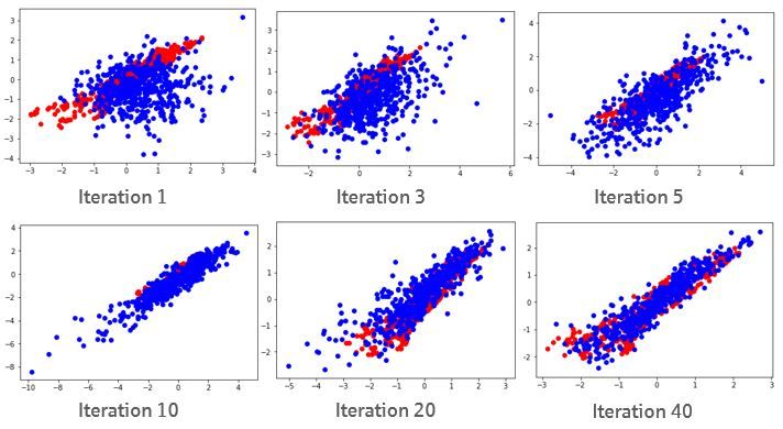
optimization and validation, we develop new performance measures and pro-
vide a consistent, assumption-free framework for the evaluation of the scenario
generation. The main properties of these evaluation measures, mainly based
on nearest-neighbour distances, are presented. Finally, we compare the results
of a GAN-based ESG to the classical ESG approach. For this comparison, we
use the benchmark portfolios created by the European Insurance and Occupa-
tional Pensions Authority (EIOPA) for the market and credit risk comparison
study (MCRCS). Those portfolios are available for asset- and liability side and
represent average exposure profiles of insurance companies in Europe. The com-
parison shows that the GAN-based ESG leads to similar results than the current
approaches used in regulatory approved internal market risk models in Europe.
In comparison to the currently used ESGs, they have the advantage that they
are assumption-free, are able to model more complex dependencies, have no
need of a time-consuming calibration process and can include new risk factors
easily.

2    Introduction
The generation of realistic scenarios how the financial markets could behave in
the future is one key component of internal market risk models used by insur-
ance companies for Solvency 2 purposes. Currently, this is done using economic
scenario generators (ESGs) which are mainly based on financial mathematical
models, see Bennemann [2011] and Pfeifer and Ragulina [2018]. These ESGs
need strong assumptions on the behaviour of the risk factors and their depen-
dencies, are time-consuming to calibrate and it is difficult in this framework to
model complex dependencies.

    An alternative method for scenario generation can be a type of neural net-
works called generative adversarial networks (GANs), invented by Goodfellow
et al. [2014]. This is a network architecture consisting of two neural networks
which has gained a lot of attention due to their ability to generate real-looking
pictures, see Aggarwal et al. [2021]. According to Motwani and Parmar [2020]
and Li et al. [2020], GANs are one of the dominant methods for the generation
of realistic and diverse examples in the domains of computer vision, image gen-
eration, image style transfer, text-to-image-translations, time-series synthesis
and natural language processing.

    As financial data, at least for liquid instruments, is consistently available,
GANs are used in various fields of finance, including market prediction, tuning
of trading models, portfolio management and optimization, synthetic data gen-
eration and diverse types of fraud detection, see Eckerli [2021]. Henry-Labordere
[2019], Lezmi et al. [2020], Fu et al. [2019], Wiese et al. [2019], Ni et al. [2020]
and Wiese et al. [2020] have already used GANs for scenario generation in the
financial sector. The focus of their reasearch was the generation of financial time
series for a limited number of risk factors (up to 6) and / or a single asset class.

                                         2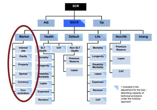
To the best of our knowledge, there is no research performing a full value-at-risk
calculation for an insurance portfolio based on these scenarios.

    The validation of the GAN performance was mainly carried out visually or
with a few statistic parameters, e.g. in Wiese et al. [2019], Ni et al. [2020] and
Wiese et al. [2020]. However, a data-driven assessment of the quality of the
generated scenarios is desirable from two points of view: to validate the model
on the basis of Solvency 2 and to optimise the hyperparameters of the GAN and
its architecture. In particular, measures based on nearest neighbor distances,
as studied by Cover and Hart [1967], Bickel and Breiman [1983], Henze [1988],
Mondal et al. [2015] and Ebner et al. [2018] seem suitable.

    In this research we
    • expand the scenario generation by a GAN to a complete risk calculation
      serving for Solvency 2 purposes in insurance companies
    • provide a consistent, assumption-free framework for the evaluation of the
      scenario generation including the evaluation of dependencies between risk
      factors and the detection of a memorizing effect
    • compare the results of a GAN-based ESG to the classical ESG approach
      implemented in regulatory approved market risk models in Europe.
The paper is structured as follows: In Section 3, we provide some background
both on market risk calculation under Solvency 2 and on GANs. Section 4 recalls
some measures from literature and presents new measures to evaluate GANs.
Additionally, we present here a framework how to combine these measures in
a hyperparameter and architecture optimization process. EIOPA annually con-
ducts a benchmarking exercise for approved market risk models in Europe, called
MCRCS. This study together with a comparison of the results of a GAN-based
ESG to the results in the study can be found in Section 5. Section 6 concludes.

3     Background
Before we present our work, we will give a short introduction to the two main
topics involved: economic scenario generators (ESG) and their use for Solvency
2 market risk calculation and generative adversarial networks (GAN).

3.1    Market risk calculation under Solvency 2
In 2016, a new regulation for insurance companies in Europe was introduced:
Solvency 2. One central requirement is the calculation of the solvency capital re-
quirement, called SCR. The SCR represents the risk of the insurer. The eligible
capital of an insurance company is then compared with the SCR to determine
whether the eligible capital is sufficient to cover the risk taken by the insurance

                                        3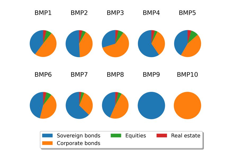
company.

    The solvency capital requirement equals the Value-at-Risk (VaR) at a 99.5%-
level for a time horizon of 1 year. A mathematical definition of the VaR and a
derivation of its usage in this context can be found in Denuit et al. [2006, p. 69].

     The risk of an insurer can be divided in different modules: market risk,
counterparty default risk, life underwriting risk, health underwriting risk, non-
life underwriting risk and operational risk. The modules themselves consist of
sub-modules, as Figure 3.1, taken from EIOPA [2014], shows:

Figure 3.1: Modules of the Solvency 2 standard formula, see EIOPA [2014, p.
6]

   The SCR can be calculated using either the standard model or an internal
model. For the standard model, the regulatory framework, European Union
[2015], sets specific rules for the calculation for each risk encountered by the
insurance company. Each internal model has to cover the same types of risks
as the standard model and must be approved by local supervisors to ensure
accordance with the principles of Solvency 2.

   In this work, we will focus on the calculation of the market risk of a non-life
insurer, covering the submodules interest rate, equity, property, spread, currency
and concentration risk. However, the methods can be applied for other risks,
too. The reason for selecting markt risk here is twofold:
   • the underlying data in the financial market is publicly available and equal
     for all insurers and

                                         4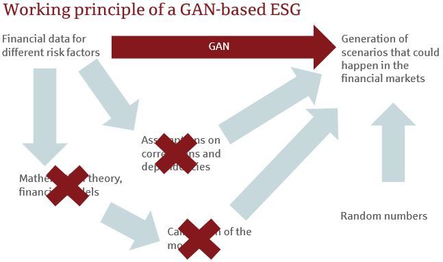
• a comprehensive benchmark exercise, called “market and credit risk com-
     parison study” MCRCS conducted by the “European Insurance and Oc-
     cupational Pensions Authority” EIOPA is available for comparison of the
     results.
We selected a non-life insurer because in contrast to a life insurer, there is no di-
rect dependency between asset and liability side. This is the case in the MCRCS
study, too. However, a GAN-based ESG can be used in the market risk calcu-
lation of a life insurer, too, as they also employ ESGs in the simulations.

    Currently, internal models for market risk often use Monte-Carlo simulation
techniques to derive the risk of the (sub)modules and then use correlations or
copulas for aggregation, see Bennemann [2011, p. 189] and Pfeifer and Rag-
ulina [2018]. The basis of the Monte-Carlo simulation is a scenario generation
performed by an “economic scenario generator” ESG. This ESG implements
financial-mathematical models for all relevant risk factors (e.g. interest rate,
equity) and their dependencies. Under those scenarios, the investment and
liabilities portfolio of the insurer is evaluated and the risk is given by the 0.5%-
percentile of the loss in these scenarios.

3.2    Generative adversarial networks
Generative adversarial networks, called GANs, are an architecture consisting of
two neural networks which are used to play a minimax-game. In 2014, GANs
were introduced by Goodfellow et al. [2014] and have gained a lot of atten-
tion afterwards because the promising results especially in image generation. A
good introduction to GANs can be found in Goodfellow et al. [2014], Goodfellow
[2016] and Chollet et al. [2018]. According to Motwani and Parmar [2020] and
Li et al. [2020], GANs are one of the dominant methods for the generation of
realistic and diverse examples in the domains of computer vision, image gen-
eration, image style transfer, text-to-image-translations, time-series synthesis,
natural language processing, etc.

    Other popular methods for the generation of data based on empirical ob-
servations are variational autoencoders and fully visible belief networks, see
Goodfellow [2016, p. 14]. However, we will use GANs here, as “GANs are gen-
erally regarded as producing better samples”, see Goodfellow [2016, p. 14].

    For the mathematical discussion in the remainder of this section, we use the
following notations:

    Let (Ω, F, P) be a probability space and d ∈ N the number of risk factors that
we model. In this research, we used a set of d = 46 risk factors. The list of those
risk factors can be found in Appendix D. E : Ω → Rd denotes the random vector
of the empirical data, the generated data by a GAN is described by the random
vector G : Ω → Rd . Let being Ej , j ∈ {1, ..., m} , m ∈ N, be independent copies

                                         5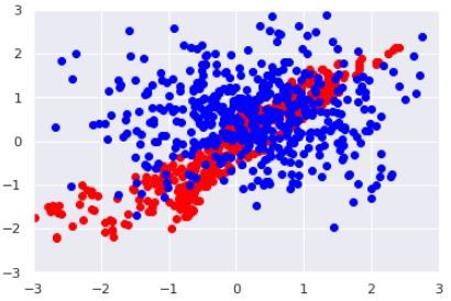
of the random vector E and Gj , j ∈ {1, ..., m} independent copies of the random
variable G. Let E(ω) = {E1 (ω), ..., Em (ω)} and G(ω) = {G1 (ω), ..., Gm (ω)} be
sets of those random variables for each ω ∈ Ω. The idea of a GAN is that
the generated data G should follow the same (but unknown) distribution as the
empirical data.
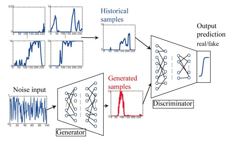
Technically, a GAN consists of two neural networks, named generator and
discriminator. The discriminator network is trained to distinguish real data-
points from “fake” datapoints and assigns every given datapoint a probability
that this datapoint is real. The input to the generator network is random noise
coming from a so called latent space. The generator is trained to produce data-
points that look like real datapoints and would be classified by the discriminator
as being real with a high probability. Picture 3.2, taken from Chen et al. [2018,
p. 2], illustrates the general architecture of a GANs training procedure:
Figure 3.2: Architecture of GANs training procedure, according to Chen et al.
[2018]
A GAN training process consists of several iterations where the weights of
both neural networks are optimised until the data from the generator is close to
the empirical/historical data. This evolution during training can be visualised
in case of a two-dimensional data distribution in Picture 3.3. The red data here
represents the empirical data to be learned whereas the blue data is generated
at the current stage of training of the generator. One can clearly see that the
generated data matches the empirical data more closely when more training
iterations of the GAN have taken place.
6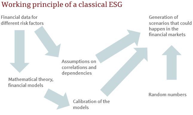
Figure 3.3: Scatterplots of the training iterations of a GAN for a two-
dimensional data distribution, red = empirical data, blue = generated data

3.3    Application of a GAN as an ESG
The strength of GANs is especially what ESGs should be good at - producing
samples of an unknown distribution based on empirical examples of that distri-
bution. Therefore, we will apply a GAN as an ESG.

    As shown in Chen et al. [2018], a GAN can be used to create new and
distinct scenarios that capture the intrinsic features of the historical data. Fu
et al. [2019, p. 3] already noted in their paper that a GAN, as a non-parametric
method, can be applied to learn the correlation and volatility structures of the
historical time series data and produce unlimited real-like samples that have
the same characteristics as the empirical observed time-series. Fu et al. [2019,
Chapter 5] have tested that this works with two stocks and calculated a 1-day
VaR.

    In our work here, we demonstrate how to expand this to a whole internal
model - with enough risk factors to model the full band-width of investments
for an insurance company and for a one year horizon as required in Solvency
2. Diagram 3.4 compares schematically the classical ESG and the idea of a
GAN-based ESG and illustrates how this simplifies the ESG process.

                                       7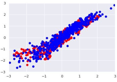
Figure 3.4: Comparison of the working principles of a classical and a GAN-based
ESG

    The main advantages of a GAN-based ESG, compared to a classical ESG,
are:

   • Assumption-free: A GAN-based ESG can be seen as being assumption-free
     as it does not contain any financial assumptions regarding distributions of
     the risk factors and their dependencies. All information on the risk factors
     stems directly from the empirically observed data. Assumptions that are
     enforced by models and that have proven to be wrong afterwards, e.g.
     the assumption of interest-rates not becoming negative that was popular
     until the financial crisis 2008/2009, can therefore not lead to a wrong
     risk-assessment.
   • Modelling of dependencies: As Denuit et al. [2006, Chapter 4] explains,
     the modelling of dependence structures beyond multivariate normality has
     become crucial in financial applications. In modern risk models, dependen-
     cies are often modelled using copulas. A certain copula has to be selected
     for each risk-factor and must be fitted so that the desired dependencies
     are reached. In practice, the modelling of dependencies is very difficult.
     In a GAN-based model, the dependencies are automatically incorporated
     from the empirical data.

   • No need for a calibration process: Calibration of the financial models to
     match the empirical data is a task that has to be performed regularly
     by risk managers to keep the models up to date. This is a cumbersome
     process and there is no standard process for calibration, see DAV [2015,
     Chapter 2.1]. This task is not needed for GAN-based models and makes
     them easier to use. If new data shall be included, the GAN simply has to
     be fed with the new data.
   • Easy integration of new risk factors: While the integration of new risk
     factors in classical ESGs often poses several issues and is quite laborious,
     in a GAN-based model, expansions of a GAN to include more risk-factors
     are straightforward.

                                       8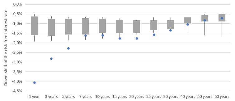
A disadvantage of a GAN-based ESG is the fact that it purely relies on events
that have happened in the past in the financial markets and cannot e.g. produce
of new dependencies that are not included in the data the model is trained with.
Classical financial models aim to derive a theory based on developments in the
past and can therefore probably produce scenarios a GAN cannot come up with.

   It is probable that a GAN-based ESG adapts faster to a regime-switch in
one of the risk factors of the model: In a classical ESG a new financial model
has to be developed and implemented, whereas a GAN has just to be trained
with new data.

4    GAN evaluation measures for GAN-based ESGs
When a GAN is used for scenario generation, the suitability of the generated
scenarios of the GAN has to be evaluated, i.e. whether the generated sce-
narios sufficiently matches the empirical observed data. This is important for
validation purposes as well as to optimize the GAN infrastructure and the hy-
perparameters of the two neural networks, generator and discriminator.

    For example, Figure 4.1 shows the results of the GAN scenario generation af-
ter only a few iterations (left) and after a sufficient amount of training iterations
(right). The red data in these figures represents the empirical data whereas the
blue resp. green points represent generated data. GAN evaluation measures
should assign a clear and robust value to each scenario generation attempt rep-
resenting the goodness-of-fit between empirical and generated data. In these
cases, the evaluation measure should assign a better value to the scenarios on
the right than to those on the left.

                                         9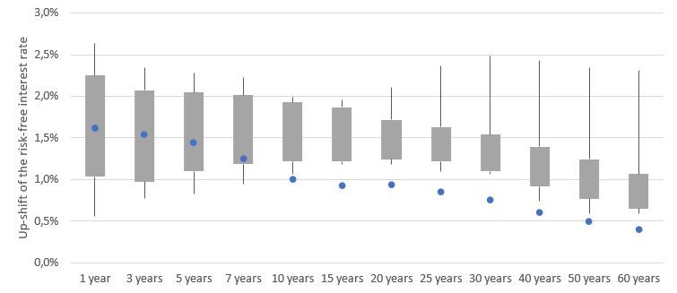
Figure 4.1: Comparison of histograms and scatterplots after a few (left) and after
sufficient (right) training iterations, red = empirical data, blue = generated data

    In this research, we employ a pure-data driven evaluation approach as one of
the main advantages of using a GAN for scenario generation is that no further
(financial-mathematical) assumptions on e.g. distributions are neccessary and
therefore we do not want to use assumptions in the evaluation. Furthermore,
we want to take measures that are easily interpretable so they can also be used
for validation purposes in Solvency 2.

   The suitability of the scenarios can be divided into three categories:

 (1) the alignment between the distributions of empirical observation and gen-
     erated data for each risk factor
 (2) the alignment of the dependencies between empiric and generated data,
     i.e. the generated points are near the empirical ones and the GAN does
     not suffer from “mode collapse”, i.e. all areas of empiric data points are
     covered by generated data points
 (3) the GAN is not “overfitted” and creates new scenarios instead of memo-
     rizing empirical ones.
These three points are discussed in Sections 4.1, 4.2 and 4.3, respectively.

                                        10
4.1 Measure for the alignment of the distributions: Wasser-
stein distance
The Wasserstein distance is commonly used to calculate the distance between
two probability distribution functions. In our case of a one dimensional issue
(empirical distribution functions for each risk factor), we can use the univariate
Wasserstein distance to calculate the distance between the two density functions
of E and G. The definition of the Wasserstein distance can be found e.g. in
Hallin et al. [2021, p. 5].
The Wasserstein distance is also known as earth-mover-distance as it can
be interpreted as the minimal amount of earth that has to be moved to trans-
form the two probability measures into each other. In terms of validation, the
Wasserstein distance in one dimension can be rewritten as a difference between
the quantile functions. Therefore, as Ramdas et al. [2017, Chapter 4.3], states
Wasserstein is a QQ-test which is often used in validation of internal models
and therefore fits for our purpose.
4.2 Measure for the alignment of the dependencies be-
tween empiric and generated data: non-covered ratio
The test on the alignment of the dependencies of the empiric and generated data
can be reformulated as a multivariate two-sample test where we want to test
the equality of two multivariate distributions based on two sets of independent
observations.
We found the following tests in literature, which can be applied in our con-
text:
• the number of statistically different bins from Richardson and Weiss [2018]
as mentioned in Borji [2019],
• nearest neighbor coincidences from Mondal et al. [2015]
• Wald-Wolfowitz two-sample test adapted from Friedman and Rafsky [1979].
We, however, propose a new measure which is easily interpretable, the non-
covered ratio. This measure is inspired by the work of Henze [1988] and Mondal
et al. [2015].
First, we want to give some illustrative understanding of the new measure
non-covered ratio which can be interpreted easily as a measure on multidimen-
sional scatterplots. The idea is that for a good fit between empirical data E and
generated data G, in every “near neighbourhood” of an empiric datapoint Ej ,
there should be a generated datapoint Gi , too, and vice versa. A data point in
11this context is defined as being in the “near neighborhood”, if it is closer than
the k-nearest neighbor of Ej out of all empirical data points. Before defining
this formally, we will have a look at an example and discuss why we will use
this measure instead of utilizing existing ones.
In the two visual examples in Figure 4.2 (for k = 1), we drew three empirical
data points Ei and three generated data points Gj . In the figures, we denoted
the 1-nearest neighbor distance of a data point Ei to all other empirical data
points by Ri .
Figure 4.2: Examples for the definition of the non-covered ratio
In the left figure, for all empirical datapoints Ei there is a generated data
point Gj which is closer that the nearest neighbor out of E. Therefore, the non-
covered ratio equals 0. In the right figure, however, all generated datapoints Gj
are further away from each Ei than the nearest neighbor out of the empirical
set. So, the non-covered ratio equals 1. As we can see, this measure is easily
interpretable and is aligned with the notion of a good match.
We decided to use the non-covered ratio instead of the other measures men-
tioned above for the following qualitative reasons. The number of statistically
different bins from Richardson and Weiss [2018] in our tests does not converge
smoothly, therefore we excluded it from our selection.
• It is the most relaxed measure in the comparison
• Areas with a bad match cannot be compensated with areas with a very
close match
Most relaxed in this context means that ith this measure more deviations be-
tween the two data sets are accepted than for the other measures. In the non-
covered ratio, there only has to exist one generated data point being inside the
k-nearest neighbor ball of Ei for this ratio to be at its minimal value. The
“nearest neighbor coincidences” test, in contrast, requires half of the generated
points to be inside the k-nearest neighbor ball of Ei to be at its minimal value.
12The Wald-Wolfowitz test is most strict: It does not only require half of the
generated data points to be inside the k-nearest neighbor ball, but it also has to
be in alternating distances for the statistic to be minimal. From a risk manage-
ment perspective a more relaxed measure is desirable because we do not want
to generate datapoints that are too close to empirical ones but give the process
some freedom to generate scenarios that have not happened in the past.
Additionally, in the “nearest neighbor coincidences” test, empirical data
points surrounded by a lot of generated points can compensate for data points
that are mostly surrounded by empirical points. This compensation can’t hap-
pen for the non covered ratio or the Wald-Wolfowitz test. As we want to have
a fitting all over the distribution, this seems more desirable.
For the formal definition of the non-covered ratio, we first have to formally
define the nearest neighbor and the nearest neighbor distance. For this, we re-
call definitions from Henze [1988], Zhou and Jammalamadaka [1993] and Ebner
et al. [2018].
Remember that in Chapter 3.2, we defined the following sets of random
variables E(ω) = {E1 (ω), ..., Em (ω)} and G(ω) = {G1 (ω), ..., Gm (ω)} for each
ω ∈ Ω representing the empirical and generated data sets. Based on this, we
define the following indices
E = {1, ..., m}
G = {m + 1, ..., 2m}
H = {1, ..., 2m}
and the random variable
(
Ei ,1 ≤ i ≤ m
Hi =
Gi−m , m + 1 ≤ i ≤ 2m
Let |.| be some norm on Rd . We take the following definition of a nearest
neighbor of a random variable from Henze [1988]:
Definition 1. Let i ∈ {1, ..., 2m}. Let r ∈ N. The k th −nearest neighbor of a
random variable Hi in the set J ⊂ {1, ..., 2m} is the random variable NkJ (Hi )
defined by
NkJ (Hi )(ω) := Hj (ω),
such that j ∈ J \ i (j depends on ω) and
∀l ∈ J \ i : |Hj (ω) − Hi (ω)| ≤ |Hl (ω) − Hi (ω)|,
if k = 1 and
|Hl (ω) − Hi (ω)| < |Hj (ω) − Hi (ω)|
for exactly k − 1 values of l, l ∈ J \ i if k > 1.
13If J = {1, .., 2m} we write Nk instead of NkJ . If ties occur where two points
have the same distance to another point, this occurs with probability zero and
can be neglected. For further discussion on this issue of ties, we refer to Schilling
[1986, p. 799] who uses a ranking in this case.
Based on this definition, we can now define the nearest neighbor distance as
in Bickel and Breiman [1983]:
Definition 2. Let i ∈ {1, ..., 2m}. Let r ∈ N. The k th −nearest neighbor
distance of Hi in the set J ⊂ {1, ..., 2m} is defined by the random variable
RkJ (Hi )(ω) = |Hi (ω) − NkJ (Hi )(ω)|
In particular, R1J (Hi )(ω) = minj∈J\i |Hi − Hj |.
With this definition, we can check for each random variable Ej if there is a
random variable out of the generated set “quite close” to it which means nearer
than the k-th nearest neighbour distance for some fixed k ∈ N. Formally, we
can define this as the non-covered ratio:
Definition 3. Let E(ω) = {E1 (ω), ..., Em (ω)} and G(ω) = {G1 (ω), ..., Gm (ω)}
for ω ∈ Ω be sets of i.i.d. random variables as above with m ∈ N. The non-
covered ratio N CRk,m of G with respect to E for the k-nearest neighbors is then
defined as
m
1 X
N CRk,m (G(ω), E(ω)) = 1 E min |Gj (ω) − Ei (ω)|
m i=1 [Rk (Ei )(ω),∞) j=1,...,m
for some k ∈ N and RkE (Ei )(ω) being the k-nearest neighbor distance of a ran-
dom variable Ei in E.
So this ratio is high if a lot of empirical data points do not have an generated
datapoint in their nearest neighbourhood. The lower the ratio, the better the
empirical data points are covered.
Analogously, one can define the measure
m
1 X
N CRk,m (E(ω), G(ω)) = 1 G min |Ej (ω) − Gi (ω)|
m i=1 [Rk (Gi )(ω),∞) j=1,...,m
For the ease of reading, we will from now on skip the ω in the formulas.
One could think of constructing a symmetric measure taking the average of
N CRk,m (G, E) and N CRk,m (E, G). We don’t do that for the following reason:
The measure N CRk,m (G, E) exactly detects “mode collapse”, the case where the
generator only produces one single value or covers only parts of the distribution
instead of generating a whole distribution. As this is an issue often occuring in
14GAN training and has to be detected and avoided, see Motwani and Parmar
[2020, Chapter 3.1] and Goodfellow [2016, Chapter 5.1.1], it is useful to have
a specialized indicator for this case. The measure N CRk,m (E, G), in contrast,
detects if there are a lot of outliers being generated that are far away from the
empirical data. If “mode collapse” occurs than the GAN architecture has to be
restructured to get better results whereas in the latter case more training itera-
tions can form a solution. Therefore, it’s useful to have a look at both measures
separately.
If the distributions of E and G are the same, the non-covered ratio converges
with the number of data points m increasing, as the following theorem shows.
To derive this result, we first have to discuss the convergence of the expected
value and the variance. For the sake of readability, we moved all proofs in the
appendix.
Lemma 4. Under the null hypothesis H0 : FG = FE , the expected value of the
non-covered ratio EH0 [N CRk,m (G, E)] converges and it holds
1
lim EH0 [N CRk,m (G, E)] = (4.1)
m→∞ 2k
Lemma 5. Under the null hypothesis H0 : FG = FE , the sequence
m · VARH0 [N CRk,m (G, E)]
converges and it holds
1 1
lim m · VARH0 [N CRk,m (G, E)] = − k
m→∞ 2k 4
This implies the convergence of the variance of the non-covered ratio
lim VARH0 [N CRk,m (G, E)] = 0 (4.2)
m→∞
With this preparatory work, we can proof the stochastical convergence of
N CRk,m (G, E) using Chebyshev’s inequality.
Theorem 6. Let N CRk,m (G, E) be the non-covered ratio as defined above and
null hypothesis H0 : FE = FG holds. Then N CRk,m (G, E) converges stochasti-
cally to 21k for m → ∞.
4.3 Measure for the detection of the memorizing effect:
memorizing ratio
All measures above will lead to optimal scores if the generated data points ex-
actly match the empirical ones, so E = G or show only tiny differences. This
is not the optimal result because we want to create new scenarios which could
have happened instead of memorizing scenarios that have actually taken place,
15see Chen et al. [2018, p. 2]. Therefore, we need a measure to detect whether
the generated data points really differ from the empirical ones and the GAN is
not simply memorizing the data points (“overfitting”).
As in a multi-dimensional space it is highly unlikely for generated and em-
pirical data points to match exactly, we extend the definition and classify a
generated datapoint Gj ∈ G as being memorized if it lays in “an unusual small
neighbourhood” around an empirical data point. We here define an “unusual
small neighbourhood” as a fraction 0 < ρ ≤ 1 of the nearest neighbour distance
of an empirical datapoint Ei ∈ E to the next empirical data point. If this is the
case for a lot of Ei ∈ E, than the generated dataset is not significantly differing
from the empirical one. The memorizing ratio then describes the proportion of
Ei ∈ E where the unwanted memorizing effect occurs.
This definition is also new to literature. The only existing test detecting
memorizing in GANs which we found in literature is the birthday paradox test,
see Borji [2019]. But this test is based on the visual identification of duplicates
for pictures and therefore cannot be utilized in our context.
Definition 7. Let ρ ∈ (0, 1]. The memorizing ratio M Rρ (E, G) is defined as:
m
1 X
M Rρ (E, G) = 1 1 min |Gj − Ei |
m i=1 [0, ρ·REi ) j=1,...,m
A graphical interpretation of the memorizing ratio can be found in Figure
4.3. In this example, En is the 1−nearest neighbor of Ei from the empirical set
E. The nearest neighbor distance between Ei and En is R = |En − Ei |. KR
then is the ball around Ei with radius R, whereas KρR forms the inner ball
around Ei with radius ρR with ρ ≤ 1. In the figure, the datapoint Gj3 counts
as a memorized data point whereas Gj1 and Gj2 are not categorized as being
memorized.
Figure 4.3: Visualization of the objects in the memorizing ratio context
16For ρ = 1, there is a simple relationship between the non-covered ratio and
the memorizing ratio and it holds:
M R1 (E, G) = 1 − N CR1,m (G, E)
It is clear that if λ% of the generated data points of G are simply memo-
rized data points from E (meaning that λ% of the realisations from G and E are
identical), then the expected value of the memorizing ratio E[M Rρ (E, G)] > λ.
So, we can use this measure to test on the memorizing effect.
Under the null hypothesis of both distributions being the same, this measure
also converges as the following theorem shows:
Theorem 8. Under the null hypothesis H0 : FG = FE , the expected value of
the memorizing ratio EH0 [M Rρ (E, G)] converges and it holds
ρd
lim EH0 [M Rρ (E, G)] =
m→∞ ρd +1
where d ∈ N is the dimension of the random vectors E and G.
This can be seen as the lower boundary of the memorizing ratio if the dis-
d
tributions are the same. Therefore, we use the difference of M Rρ (E, G) − ρdρ+1
for evaluation.
To check for the convergence empirically, we conducted a two-sample test
for different values of ρ in various dimensions and with the same distribution for
both samples. We conducted this test with different distributions (e.g. normal,
exponential, student-t). We calculated the value of the memorizing ratio then
for an increasing number of data points in each sample. Figure 4.4 presents the
test for 2 dimensions, normal distributions and three different values for ρ.
17Figure 4.4: Convergence test for the memorizing ratio
d
As expected, the memorizing ratio always converges to ρdρ+1 . To derive the
convergence speed, we can use the following definition from Leisen and Reimer
[1996] :
Definition 9. A sequence of errors N converges with order α > 0, if there is a
constant κ > 0 such that
κ
∀N ∈ N : N ≤ α
N
The order of convergence can be determined by simulation if we use, as in
Leisen and Reimer [1996] or Junike [2019, Chapter 18.6], the transformation
κ
log( ) = log(κ) − α log(N )
Nα
and perform a linear regression on the log-log-scale based on the data from the
convergence test above. In our tests, we found the order of convergence to be
between 0.02 and 0.6, strongly depending on ρ. The order of convergence is
very low if ρ is small. Therefore, we suggest to use a value of at least 0.5 for ρ.
4.4 Hyperparameter optimization using these evaluation
measures
In the preceeding sections, we determined a combination of Wasserstein dis-
tance for each risk factor wi , i = 1, ..., d, both variants of the non-covered ratio
N CRk,m (E, G) (abbr. ncr_b) and N CRk,m (G, E) (abbr. ncr_o) and the mem-
orizing ratio M Rρ (E, G) (abbr. mr) being useful to determine the quality of
the GAN results.
18We now want to use these evaluation measures to optimize the hyperparam-
eters of the two neural networks and the GAN infrastructure itself. In a GAN,
there is a lot of different variants to be tested. A full optimization is not pos-
sible as, see Motwani and Parmar [2020, Chapter 2], the “selection of the GAN
model for a particular application is a combinatorial exploding problem with a
number of possible choices and their orderings. It is computationally impossible
for researchers to explore the entire space.“ So, in our work, we check on the
following:
• Number of layers for generator and discriminator: Not only the number
itself, but also the relation between the number of layers in each neural
network can make a big difference.
• Number of neurons per layer: This, too, can be different between the two
neural networks and can also vary from layer to layer inside a network.
• Number of training iterations of the generator versus discriminator: The
discriminator is usually trained k times in each iteration where the gener-
ator is trained once. We will check for an optimal parameter k.
• Dimension of the latent space: The latent space where the input for the
generator is sampled usually has a higher dimensionality than the dimen-
sion of the generators’ output.
• Functions used in the GAN: The activation functions in the layers of the
two networks, the optimisation algorithm and the usage of batch normal-
isation can be varied.
We performed our tests for d=46 dimensions and with the parameters k = 3
and ρ = 0.7. The data used was derived from the MCRCS study conducted by
EIOPA (see EIOPA MCRCS Project Group [2020b]) and will be further dis-
cussed in Chapter 5.
Figure 4.5 shows the development of the Wasserstein distances for all 46
risk factors and the development of the other three measures with both neural
networks having 4 layers over the 2500 training iterations:
19Figure 4.5: Development of the chosen GAN evaluation measures for the GAN
with (4,4)-layer configuration
In the right figure, one can clearly see the behaviour of the memorizing ratio
serving as a opponent to the non-covered ratio: Over the training iterations,
the data distributions get closer and closer, and therefore the non-covered ra-
tio decreases near to its expected value of 213 . The memorizing ratio, however,
increases with more training iterations. The expected value of the memorizing
0.746
ratio in this case is close to zero ( 0.7 46 +1 ≈ 10
−8
). In this configuration, about
a fifth of the data points at the end of the training is classified as being memo-
rized. However, a large number of memorized points is undesirable. Therefore,
the omittance of this ratio would lead to the selection of a non-optimal GAN
architecture.
To derive at one value for the total performance of the GAN architecture
in question, we have to aggregate the values from the four measures in each
evaluation run. Our experience shows that simply taking the average of the
four measures as the target function tf works well. In other contexts, it can
make sense to introduce some kind of weighting in this formula.
1 1 1 ρd
tf = max (wi ) + ncr_o − k + ncr_b − k + max(mr − d , 0)
4 i=1,...,46 2 2 ρ +1
The measures for the differences between joint distributions (ncr_b and
ncr_o) and mr can be evaluated in a space with the same dimension as the
input parameters, so one figure per measure is obtained. For ncr_o and ncr_b,
we subtract the expected value under the null hypothesis of equal distributions
and take the absolute value. For mr, we take the maximum of the absolute value
of the difference between mr and their expected value under the null hypothesis
and 0 because lower values for mr mean a lower amount of memorized data
points which is not only accepted but appreciated. The Wasserstein distance,
however, is detemined for each risk factor, in our case leading to 46 figures. To
aggregate, we will use the maximum over this 46 risk factors, leading to one
figure for Wasserstein, too.
20Figure 4.6 demonstrates the development of the tf-value over the training
iterations for a configuration with both neural networks having 4 layers. As
it is computationally expensive to calculate this tf −value in every iteration of
the GAN training, we decide to determine the tf −value every 25 training iter-
ations where 25 is a compromise between accuracy and computational feasibility.
Figure 4.6: Development of the tf -value for a GAN with a (4,4)-layer configu-
ration
Based on the tf −value, one can then select not only the best architecture,
but also the optimal number of training iterations.
In the experiments, one can clearly see that the GAN is not converging but
there is a minimum of the target function during training and afterwards the
tf -value starts increasing again. This is the behaviour typically seen in GAN
training, see e.g. Goodfellow [2016, p. 34]. Figure 4.7 displays the Wasserstein
(left) and ncr_o/ncr_b/mr-measures (right) for a run with 5000 iterations:
21Figure 4.7: Development of the chosen GAN evaluation measures over 5000
training iterations
Based on our analysis of 50 different settings, we use the following configu-
ration for our GAN-based ESG:
• 4 layers for discriminator and generator
• 400 neurons per layer in the discriminator and 200 in the generator
• 10 training iterations for the generator in each discriminator training
• Dimension of the latent space is 200
• We use LeakyReLu as activation functions, except for the output layers
which use sigmoid (for discriminator) and linear (for generator) activiation
functions. We use the Adam optimizer and batch normalisation after each
of the layers in the network.
For this GAN, we check at which iteration the tf -value is minimized. In our
case, this is iteration 2425. Then we use the trained generator at this iteration
to generate the scenarios for our comparison with the results of classical ESGs
in the next chapter.
5 Comparison of GAN results with the results of
the MCRCS study
5.1 Introduction to the MCRCS study
Since 2017, the “European Insurance and Occupational Pensions Authority”
EIOPA performs an annual study, called the market and credit risk comparison
study, abbr. "MCRCS". According to the instructions from EIOPA MCRCS
Project Group [2020b], the "primary objective of the MCRCS is to compare
market and credit risk model outputs for a set of realistic asset portfolios".
In the study, all insurance undertakings with significant exposure in EUR and
with an approved internal model are asked to participate, see EIOPA MCRCS
22Project Group [2021]. In the study as of year-end 2019, 21 insurance companies
from 8 different countries of the European Union participated.
All participants are asked by their local regulators to model the risk of
104 different synthetic instruments. Those comprise all relevant asset classes,
i.e. risk-free interest rates, sovereign bonds, corporate bonds, foreign exchange
rates, equity indices, property, foreign exchange and some derivatives. A de-
tailed overview of the synthetic instruments that are used in this study can be
found in EIOPA MCRCS Project Group [2020a].
Additionally, those instruments are grouped into 10 different asset-only bench-
mark portfolios, 2 liability-only benchmark portoflios and 10 combined portfo-
lios. These portfolios "should reflect typical asset risk profiles of European
insurance undertakings", see EIOPA MCRCS Project Group [2020b, Section
2]. This analysis sheds light into the interaction and dependencies between the
risk factors. Figure 5.1 presents the asset-type composition of the asset-only
benchmark portfolios.
Figure 5.1: Composition of the MCRCS benchmark portfolios BMP1 - BMP10
All asset portfolios mainly consist of fixed income securities (86% to 94%) as
this forms the main investment focus of insurance companies. However, there
are significant differences both in ratings, durations and also in the weighting
between sovereign and corporate exposures. The two liability profiles are as-
sumed to be zero-bond based, so they represent a non-life insurance companies’
liabilities and differ in their durations (13.1 years vs. 4.6 years).
235.2 Methodology and data
For the purpose of this article, we will only compare the risk charges for instru-
ments that are also included in the benchmark portfolios. An aggregated view
of these instruments together with the used Bloomberg sources can be found in
Appendix D. As the study used here is at year-end 2019, we take the datapool
from end of March 2002 until Dec. 2019 as the basis of our GAN training. We
therefore have 4587 daily observations in this dataset which comprises almost
18 years.
In Solvency 2, we have to model the market risk for a one year horizon.
There are two approaches to derive the risk based on higher frequent data (here
daily returns) for a longer horizon (here annually). One solution is to use the
daily data to train the GAN model and then use some autocorrelation function
to generate an annual time series based on daily returns. The other solution
is to use overlapping rolling windows of annual returns on a daily basis for the
training of the model. The first method is covered in Fu et al. [2019]. We will
in this work use overlapping rolling windows as explained in Wiese et al. [2020,
p. 16] and EIOPA MCRCS Project Group [2021, p. 17].
Annually, EIOPA provides a detailed study with a comparison of the results
by BMP, instruments and some additional analysis, e.g. for the analysis of de-
pendencies for the risk factors. The study for year-end 2019 can be found on
the EIOPA homepage, see EIOPA MCRCS Project Group [2021]. There, the
risk charges are compared between the participating insurance companies in an
anonymized way.
5.3 Comparison on risk-factor level
The results on risk factor basis are analyzed based on the shocks generated or
implied by the ESGs. A shock hereby is defined in EIOPA MCRCS Project
Group [2021, p. 11] as
Definition 10. A shock is the absolute change of a risk factor over a one-year
time horizon. Depending on the type of risk factor, the shocks can either be two-
sided (e.g. interest rates ‘up/down’) or one-sided (e.g. credit spreads ‘up’). This
metric takes into account the undertakings’ individual risk measure definitions
(in particular whether the mean of the distribution is taken into account or not)
and is based on the 0.5% and 99.5% quantiles for two-sided risk factors and the
99.5% quantile for one-sided risk factors, respectively.
The results are presented in one diagram, showing boxes with whiskers for
each maturity / sub-type of this risk factor. The boxes contain the shocks of
the participating insurance companies between the 25%- and 75%-percentile of
all participants. The whiskers extend this to the 10%- and 90%-percentile. The
sample consists of 21 participants at maximum; results are only provided if an
24insurance company states at least some exposure to this risk-factor.
We enrich those results with a blue dot representing the shock for that risk
factor generated by our GAN-based model. In this work, we will show the
comparison of the four most important risk factor shocks (interest rate up and
down, credit spread and equity).
Figure 5.2: Comparison of the simulated shifts for the credit spread and equity
risk factors, representation based on own results and EIOPA MCRCS Project
Group [2021, p. 25 and 27]
For credit spreads and equity, Figure 5.2, we see a good alignment between
the GAN-based model and the approved internal models. On the equity side,
the alignment is also good for most of the risk factors. For the FTSE100, the
GAN produces less severe shocks than the other models. This behaviour, how-
ever, can actually be found in the training data as the FTSE100 is less volatile
than the other indizes for the time frame used in GAN training. So, the GAN
here produces plausible results.
For interest rates, however, the picture is more complex as Figure 5.3 illus-
trates:
Figure 5.3: Comparison of the simulated shifts for the most important risk
factors, representation based on own results and EIOPA MCRCS Project Group
[2021, p. 22]
The up-shifts generated by the GAN-based model are within the boxes (25%-
percentile to 75%-percentile of the participating internal models) for 1 to 7 year
25buckets. Afterwards, the shifts are below the whiskers. This effect is probably
due to the time span of the data used for the training of the GAN. The interest
rates in this time period (Mar. 2002 - Dec. 2019) are mostly decreasing. In the
traditional ESGs, the interest rates are probably calibrated on a longer horizon
so they include upward trends in long term interest rates from a longer history.
We use this time horizon in our GAN training since the availability of consistent
market data gets more difficult if one goes further back in history.
For the down-shifts, the graph shows a contrary behaviour: The short- and
medium term interest rates are far below the whiskers, whereas the longer term
interest rates mostly are inside the whiskers or boxes. This also can be explained
by the interest rate development: The time span used for training of the GAN
shows a sharp decrease of interest rates especially in the short term whereas
longer term interest rates behaved more stable. This behaviour is mimicked by
the GAN. In traditional ESGs, additionally to the longer time span used for
calibration, often expert judgement by the insurers leads to a lower bound on
how negative interest rates can become.
If an insurance company wants to include more up-shifts in the training, the
training data has to be transformed accordingly. This, however, would deviate
from the idea of the GAN-based ESG as a full data-driven model. Addition-
ally, it is a valid point to discuss whether the interest rate movements having
occurred in a different regime with much higher interest rates are meaningful
for the fluctuations in a current low interest rate environment.
5.4 Comparison on portfolio level
The main comparison between the results for the the benchmark portfolios is
based on the "risk charge" which is defined in EIOPA MCRCS Project Group
[2020b, Section 2].
Definition 11. The risk charge is the ratio of the modelled Value at Risk
(99.5%, one year horizon) and the provided market value of the portfolio.
In this work, we only show the comparison of the risk charges for the
combined asset-and-liabilities portfolios. The comparisons for asset-only and
liability-only benchmark portfolios follow a similiar pattern.
Figure 5.4 displays for each of the benchmark portfolios which comprises the
longer liability structure (left) or the shorter liabilities (right) the risk charge of
this portfolio. As in the comparison for the risk factors, the grey boxes contain
the risk charges of the participating insurance companies between the 25%- and
75%-percentile. The whiskers extend this to the 10%- and 90%-percentile. The
sample consists of 21 participants, so 4 results (2 above, 2 below the whiskers)
are not shown. The risk charge according to our GAN-based model is repre-
26sented by a blue dot.
Figure 5.4: Comparison of the combined asset-liability benchmark portfolios,
representation based on own results and EIOPA MCRCS Project Group [2021,
p. 14]
The risk charge of the GAN-based model fits well to the risk charges of the
established models. On the left side (longer liability structure), the blue dot
always is in the upper percentile of the risk charges or slightly above the 90%-
percentile. Due to the asset-liability duration profile in this portfolio, the risk
charge is generated by scenarios witrh decreasing interest rates. In the risk fac-
tor comparison of the interest rate down shock, the interest rate down shifts are
more severe in most maturities for the GAN-based model than for the classical
models. Therefore, it seems plausible for the resulting portfolio risk to be at the
upper percentiles, too.
The right graph (shorter liability structure) shows a bit a different picture:
The risk charge of the GAN-based model mostly lies within the boxes or within
the lower whiskers. This is due to the fact that for this portfolio structure,
increasing interest rates form a main risk. As the shocks for the GAN-based
model for increasing interest rates are within the boxes or even below the boxes,
this behaviour can be explained, too.
Overall, the resulting risk charges for the GAN-based model are comparable
to the results of the approved internal models in Europe. Therefore, GAN-based
models can be seen as an appropriate alternative way of market risk modelling.
6 Summary and Conclusion
In this research, we have shown how a generative adversarial network (GAN)
can serve a an economic scenario generator (ESG). Compared to the current
approaches, a GAN-based ESG is an assumption-free approach that can model
complex dependencies between risk factors.
27For validation purposes as well as for the optimization of the GAN itself,
we provided three measures that can evaluate the performance of the scenario
generation of the GAN: Wasserstein distance (measuring the alignment of the
distributions of the risk factors), non-covered ratio (measuring the alignment of
the dependencies between the risk factors and controlling mode-collapse) and
the memorizing ratio (measuring overfitting). We provided a framework how
these measures can be used in the hyperparameter and GAN architecture opti-
mization process.
Finally, we showed that the results of a GAN-based ESG are comparable to
the currently used ESGs when using the EIOPA MCRCS study as a benchmark.
Acknowledgement 12. S. Flaig would like to thank Deutsche Rückversicherung
AG for the funding of this research. Opinions, errors and omissions are solely
those of the authors and do not represent those of Deutsche Rückversicherung
AG or its affiliates.
References
Alankrita Aggarwal, Mamta Mittal, and Gopi Battineni. Generative adversarial
network: An overview of theory and applications. International Journal of
Information Management Data Insights, page 100004, 2021.
Christoph Bennemann. Handbuch Solvency II: von der Standardformel zum
internen Modell, vom Governance-System zu den MaRisk VA. Schäffer-
Poeschel, 2011.
Peter J Bickel and Leo Breiman. Sums of functions of nearest neighbor distances,
moment bounds, limit theorems and a goodness of fit test. The Annals of
Probability, pages 185–214, 1983.
Ali Borji. Pros and cons of gan evaluation measures. Computer Vision and
Image Understanding, 179:41–65, 2019.
Yize Chen, Pan Li, and Baosen Zhang. Bayesian renewables scenario generation
via deep generative networks. In 2018 52nd Annual Conference on Informa-
tion Sciences and Systems (CISS), pages 1–6. IEEE, 2018.
Francois Chollet et al. Deep learning with Python, volume 361. Manning New
York, 2018.
Thomas Cover and Peter Hart. Nearest neighbor pattern classification. IEEE
transactions on information theory, 13(1):21–27, 1967.
DAV. Zwischenbericht zur Kalibrierung und Validierung spezieller ESG unter
Solvency II. Ergebnisbericht des Ausschusses Investment der Deutschen
Aktuarvereinigung e.V., 2015. URL https://aktuar.de/unsere-themen/
28fachgrundsaetze-oeffentlich/2015-11-09_DAV-Ergebnisbericht_
Kalibrierung_und_Validierung_spezieller_ESG_Update.pdf.
Michel Denuit, Jan Dhaene, Marc Goovaerts, and Rob Kaas. Actuarial theory
for dependent risks: measures, orders and models. John Wiley & Sons, 2006.
Bruno Ebner, Norbert Henze, and Joseph E Yukich. Multivariate goodness-
of-fit on flat and curved spaces via nearest neighbor distances. Journal of
Multivariate Analysis, 165:231–242, 2018.
Florian Eckerli. Generative adversarial networks in finance: an overview. Avail-
able at SSRN 3864965, 2021.
EIOPA. The underlying assumptions in the standard formula for the solvency
capital requirement calculation. the European Insurance and Occupational
Pensions Authority, 2014.
EIOPA MCRCS Project Group. 13.01.2020_MCRCS 2019 instruments and
BMP.xlsx, 2020a. URL https://www.eiopa.europa.eu/sites/default/
files/toolsanddata/mcrcs_2019_instruments_and_bmp.xlsx.
EIOPA MCRCS Project Group. YE2019 Comparative Study on Market and
Credit Risk Modelling, 2020b. URL https://www.eiopa.europa.eu/sites/
default/files/toolsanddata/mcrcs_year-end_2019_instructions_
covidpostponed.pdf.
EIOPA MCRCS Project Group. YE2019 Comparative Study on
Market and Credit Risk Modelling, 2021. URL https://www.
eiopa.europa.eu/sites/default/files/publications/reports/
2021-study-on-modelling-of-market-and-credit-risk-_mcrcs.pdf.
European Union. Commission delegated regulation (EU) 2015/35 of 10 October
2014 supplementing directive 2009/138/EC of the European parliament and
of the council on the taking-up and pursuit of the business of insurance and
reinsurance (Solvency II). Official Journal of European Union, 2015.
Jerome H Friedman and Lawrence C Rafsky. Multivariate generalizations of the
wald-wolfowitz and smirnov two-sample tests. The Annals of Statistics, pages
697–717, 1979.
Rao Fu, Jie Chen, Shutian Zeng, Yiping Zhuang, and Agus Sudjianto. Time
series simulation by conditional generative adversarial net. arXiv preprint
arXiv:1904.11419, 2019.
Ian Goodfellow. Nips 2016 tutorial: Generative adversarial networks. arXiv
preprint arXiv:1701.00160, 2016.
Ian Goodfellow, J. Pouget-Abadie, and M. et al Mirza. Generative adversarial
nets. Advances in neural information processing systems, pages 2672–2680,
2014.
29Marc Hallin, Gilles Mordant, and Johan Segers. Multivariate goodness-of-fit
tests based on wasserstein distance. Electronic Journal of Statistics, 15(1):
1328–1371, 2021.
Pierre Henry-Labordere. Generative models for financial data. Available at
SSRN 3408007, 2019.
Norbert Henze. A multivariate two-sample test based on the number of nearest
neighbor type coincidences. The Annals of Statistics, 16(2):772–783, 1988.
Gero Quintus Rudolf Junike. Advanced stock price models, concave distortion
functions and liquidity risk in finance. 2019.
Dietmar PJ Leisen and Matthias Reimer. Binomial models for option valuation-
examining and improving convergence. Applied Mathematical Finance, 3(4):
319–346, 1996.
Edmond Lezmi, Jules Roche, Thierry Roncalli, and Jiali Xu. Improving the
robustness of trading strategy backtesting with boltzmann machines and gen-
erative adversarial networks. Available at SSRN 3645473, 2020.
Ziqiang Li, Rentuo Tao, and Bin Li. Regularization and normalization for
generative adversarial networks: A review. arXiv preprint arXiv:2008.08930,
2020.
Pronoy K Mondal, Munmun Biswas, and Anil K Ghosh. On high dimensional
two-sample tests based on nearest neighbors. Journal of Multivariate Analy-
sis, 141:168–178, 2015.
Tanya Motwani and Manojkumar Parmar. A novel framework for selection of
gans for an application. arXiv preprint arXiv:2002.08641, 2020.
Hao Ni, Lukasz Szpruch, Magnus Wiese, Shujian Liao, and Baoren Xiao.
Conditional sig-wasserstein gans for time series generation. arXiv preprint
arXiv:2006.05421, 2020.
Dietmar Pfeifer and Olena Ragulina. Generating VaR scenarios under Solvency
II with product beta distributions. Risks, 6(4):122, 2018.
Aaditya Ramdas, Nicolás García Trillos, and Marco Cuturi. On wasserstein
two-sample testing and related families of nonparametric tests. Entropy, 19
(2):47, 2017.
Eitan Richardson and Yair Weiss. On gans and gmms. arXiv preprint
arXiv:1805.12462, 2018.
Mark F Schilling. Multivariate two-sample tests based on nearest neighbors.
Journal of the American Statistical Association, 81(395):799–806, 1986.
30You can also read