Fanaroff-Riley classification of radio galaxies using group-equivariant convolutional neural networks.

MNRAS 000, 1–11 (2015) Preprint 19 February 2021 Compiled using MNRAS LATEX style file v3.0

 Fanaroff-Riley classification of radio galaxies using group-equivariant
 convolutional neural networks.
 Anna M. M. Scaife,1,2★ and Fiona Porter1
 1 Jodrell Bank Centre for Astrophysics, Department of Physics & Astronomy, University of Manchester, Oxford Road, Manchester M13 9PL UK
 2 The Alan Turing Institute, Euston Road, London NW1 2DB, UK

 Accepted XXX. Received YYY; in original form ZZZ
arXiv:2102.08252v2 [astro-ph.IM] 18 Feb 2021

 ABSTRACT
 Weight sharing in convolutional neural networks (CNNs) ensures that their feature maps will be translation-equivariant. However,
 although conventional convolutions are equivariant to translation, they are not equivariant to other isometries of the input image
 data, such as rotation and reflection. For the classification of astronomical objects such as radio galaxies, which are expected
 statistically to be globally orientation invariant, this lack of dihedral equivariance means that a conventional CNN must learn
 explicitly to classify all rotated versions of a particular type of object individually. In this work we present the first application of
 group-equivariant convolutional neural networks to radio galaxy classification and explore their potential for reducing intra-class
 variability by preserving equivariance for the Euclidean group E(2), containing translations, rotations and reflections. For the
 radio galaxy classification problem considered here, we find that classification performance is modestly improved by the use
 of both cyclic and dihedral models without additional hyper-parameter tuning, and that a 16 equivariant model provides the
 best test performance. We use the Monte Carlo Dropout method as a Bayesian approximation to recover epistemic uncertainty
 as a function of image orientation and show that E(2)-equivariant models are able to reduce variations in model confidence as a
 function of rotation.
 Key words: radio continuum: galaxies – methods: data analysis – techniques: image processing

 1 INTRODUCTION Network; Wu et al. 2018) model made use of the Faster R-CNN (Ren
 et al. 2015) network to identify and classify radio sources; Alger
 In radio astronomy, a massive increase in data volume is currently
 et al. (2018) made use of an ensemble of classifiers including CNNs
 driving the increased adoption of machine learning methodologies
 to perform host galaxy cross-identification. Tang et al. (2019) made
 and automation during data processing and analysis. This is largely
 use of transfer learning with CNNs to perform cross-survey classifi-
 due to the high data rates being generated by new facilities such
 cation, while Gheller et al. (2018) made use of deep learning for the
 as the Low-Frequency Array (LOFAR; Van Haarlem et al. 2013),
 detection of cosmological diffuse radio sources. Lukic et al. (2018)
 the Murchison Widefield Array (MWA; Beardsley et al. 2019), the
 also performed morphological classification using a novel technique
 MeerKAT telescope (Jarvis et al. 2016), and the Australian SKA
 known as capsule networks (Sabour et al. 2017), although they found
 Pathfinder (ASKAP) telescope (Johnston et al. 2008). For these in-
 no specific advantage compared to traditional CNNs. Bowles et al.
 struments a natural solution has been to automate the data processing
 (2020) showed that an attention-gated CNN could be used to per-
 stages as much as possible, including classification of sources.
 form Fanaroff-Riley classification of radio galaxies with equivalent
 With the advent of such huge surveys, new automated classification
 performance to other applications in the literature, but using ∼50%
 algorithms have been developed to replace the “by eye” classifica-
 fewer learnable parameters than the next smallest classical CNN in
 tion methods used in earlier work. In radio astronomy, morphological
 the field.
 classification using convolutional neural networks (CNNs) and deep
 Convolutional neural networks classify images by learning the
 learning is becoming increasingly common for object classification,
 weights of convolutional kernels via a training process and using
 in particular with respect to the classification of radio galaxies. The
 those learned kernels to extract a hierarchical set of feature maps
 ground work in this field was done by Aniyan & Thorat (2017) who
 from input data samples. Convolutional weight sharing makes CNNs
 made use of CNNs for the classification of Fanaroff-Riley (FR) type
 more efficient than multi-layer perceptrons (MLPs) as it ensures
 I and type II radio galaxies (Fanaroff & Riley 1974). This was fol-
 translation-equivariant feature extraction, i.e. a translated input signal
 lowed by other works involving the use of deep learning in source
 results in a corresponding translation of the feature maps. However,
 classification. Examples include Lukic et al. (2018) who made use of
 although conventional convolutions are equivariant to translation,
 CNNs for the classification of compact and extended radio sources
 they are not equivariant to other isometries of the input data, such
 from the Radio Galaxy Zoo catalogue (Banfield et al. 2015), the
 as rotation, i.e. rotating an image and then convolving with a fixed
 CLARAN (Classifying Radio Sources Automatically with a Neural
 filter is not the same as first convolving and then rotating the re-
 sult. Although many CNN training implementations use rotation as
 ★ E-mail: anna.scaife@manchester.ac.uk (AMS) a form of data augmentation, this lack of rotational equivariance

 © 2015 The Authors

2 A. M. M. Scaife & F. Porter
means that a conventional CNN must explicitly learn to classify all rics, and introduce a novel use of the Monte Carlo Dropout method
rotational augmentations of each image individually. This can result for quantitatively assessing the degree of model confidence in a test
in CNNs learning multiple copies of the same kernel but in different prediction as a function of image orientation; in Section 6 we discuss
orientations, an effect that is particularly notable when the data itself the validity of the assumptions that radio galaxy populations are ex-
possesses rotational symmetry (Dieleman et al. 2016). Furthermore, pected to be staitsically rotation and reflection unbiased and review
while data augmentation that mimicks a form of equivariance, such as the implications of this work in that context; in Section 7 we draw
image rotation, can result in a network learning approximate equiv- our conclusions.
ariance if it has sufficient capacity, it is not guaranteed that invariance
learned on a training set will generalise equally well to a test set (Lenc
& Vedaldi 2014). A variety of different equivariant networks have 2 E(2)-EQUIVARIANT G-STEERABLE CNNS
been developed to address this issue, each guaranteeing a particular
transformation equivariance between the input data and associated Group CNNs define feature spaces using feature fields : R2 → R ,
feature maps. For example, in the field of galaxy classification using which associate a -dimensional feature vector ( ) ∈ R to each
optical data, Dieleman et al. (2015) enforced discrete rotational in- point of an input space. Unlike conventional CNNs, the feature
variance through the use of a multi-branch network that concatenated fields of such networks contain transformations that preserve the
the output features from multiple convolutional branches, each using transformation law of a particular group or subgroup, which allows
a rotated version of the same data sample as its input. However, while them to encode orientation information. This means that if one trans-
effective, the approach of Dieleman et al. (2015) requires the con- forms the input data, , by some transformation action, , (translation,
volutional layers of a network architecture and hence the number of rotation, etc.) and passes it through a trained layer of the network,
model weights associated with them to be replicated times, where then the output from that layer, Φ( ), must be equivalent to having
 is the number of discrete rotations. passed the data through the layer and then transformed it, i.e.
 Recently, a more efficient method of using convolutional layers that Φ(T ) = T 0 Φ( ), (1)
are equivariant to a particular group of transforms has been devel-
oped, which requires no replication of architecture and hence fewer where T is the transformation for action . In the case where the
learnable parameters to be used. Explicitly enforcing an equivariance transformation is invariant rather than equivariant, i.e. the input
in the network model in this way not only provides a guarantee that does not change at all when it is transformed, T 0 will be the identity
it will generalise, but also prevents the network using parameter ca- matrix for all actions ∈ . In the case of equivariance, T does
pacity to learn characteristic behaviour that can instead be specified not necessarily need to be equal to T 0 and instead must only fulfil
a priori. First introduced by Cohen & Welling (2016), these Group the property that it is a linear representation of , i.e. T ( ℎ) =
equivariant Convolutional Neural Networks (G-CNNs), which pre- T ( )T (ℎ).
serve group equivariance through their convolutional layers, are a Cohen & Welling (2016) demonstrated that the conventional con-
natural extension of conventional CNNs that ensure translational in- volution operation in a network can be re-written as a group convo-
variance through weight sharing. Group equivariance has also been lution:
demonstrated to improve generalisation and increase performance ∑︁ ∑︁
 [ ∗ ] ( ) = (ℎ) ( −1 ℎ), (2)
(see e.g. Weiler et al. 2017; Weiler & Cesa 2019). In particular,
 ℎ ∈ 
Steerable G-CNNs have become an increasingly important solution
to this problem and notably those steerable CNNs that describe E(2)- where = R2 in layer one and = in all subsequent layers. Whilst
equivariant convolutions. this operation is translationally-equivariant, is still rotationally
 The Euclidean group E(2) is the group of isometries of the plane R2 constrained. For E(2)-equivariance to hold more generally, the kernel
that contains translations, rotations and reflections. Isometries such as itself must satisfy
these are important for general image classification using convolution
 ( ) = out ( ) ( ) in ( −1 ) ∀ ∈ , ∈ R2 , (3)
as the target object in question is unlikely to appear at a fixed position
and orientation in every test image. Such variations are not only (Weiler et al. 2018), where is an action from group , and :
highly significant for objects/images that have a preferred orientation, R2 → R in × out , where in and out are the number of channels in
such as text or faces, but are also important for low-level features in the input and output data, respectively; is the group representation,
nominally orientation-unbiased targets such as astrophysical objects. which specifies how the channels of each feature vector mix under
In principle, E(2)-equivariant CNNs will generalize over rotationally- transformations. Kernels which fulfil this constraint are known as
transformed images by design, which reduces the amount of intra- rotation-steerable and must be constructed from a suitable family of
class variability that they have to learn. In effect such networks are basis functions. As noted above, this is a linear relationship, which
insensitive to rotational or reflection variations and therefore learn means that G-steerable kernels form a subspace of the convolution
only features that are independent of these properties. kernels used by conventional CNNs.
 In this work we introduce the use of -steerable CNNs to as- For planar images the input space will be R2 , and for single fre-
tronomical classification. The structure of the paper is as follows: quency or continuum radio images these feature fields will be scalar,
in Section 2 we describe the mathematical operation of -steerable such that : R2 → R. The group representation for scalar fields is
CNNs and define the specific Euclidean subgroups being consid- also known as the trivial representation, ( ) = 1 ∀ ∈ , indicat-
ered in this work; in Section 3 we describe the data sets used in ing that under a transformation there is no orientation information
this work and the preprocessing steps implemented on those data; in to preserve and that the amplitude does not change. The group rep-
Section 4 we describe the network architecture adopted in this work, resentation of the output space from a G-steerable convolution must
explain how the -steerable implementation is constructed and spec- be chosen by the user when designing their network architecture and
ify the group representations; in Section 5 we give an overview of can be thought of as a variety of hyper-parameter.
the training outcomes including a discussion of the convergence for However, whilst the representation of the input data is in some
different equivalence groups, validation and test performance met- senses quite trivial for radio images, in practice convolution layers are

MNRAS 000, 1–11 (2015)

E(2)-equivariant radio galaxy classification 3
interleaved with other operations that are sensitive to specific choices Digit 1 Digit 2 Digit 3
of representation. In particular, the range of non-linear activation
layers permissible for a particular group or subgroup representation 0 - FRI 0 - Confident 0 - Standard
may be limited. Trivial representations, such as scalar fields, do not 1 - FRII 1 - Uncertain 1 - Double-double
transform under rotation and therefore conventional nonlinearities 2 - Hybrid 2 - Wide-angle Tail
like the widely used ReLU activation function are fine. Bias terms 3 - Unclassifiable 3 - Diffuse
 4 - Head-tail
in convolution allow equivariance for group convolutions only in
the case where there is a single bias parameter per group feature
 Table 1. Numerical identifiers from the catalogue of Miraghaei & Best (2017).
map (rather than per channel feature map) and likewise for batch
normalisation (Cohen & Welling 2016).
 In this work we use the G-steerable network layers from Weiler
& Cesa (2019) who define the Euclidean group as being con- We note that not all combinations of the three digits described in
structed from the translation group, (R, +), and the orthogonal group, Table 1 are present in the catalogue as some morphological classes
O(2) = { ∈ R2×2 | = id2×2 }, such that the Euclidean are dependent on the parent FR class, with only FRI type objects be-
group is congruent with the semi-direct product of these two groups, ing sub-classified into head-tail or wide-angle tail, and only FRII type
E(2)  (R, +)o O(2). Consequently, the operations contained in the objects being sub-classified as double-double. Hybrid FR sources are
orthogonal group are those which leave the origin invariant, i.e. not considered to have any non-standard morphologies, as their stan-
continuous rotations and reflections. In this work we specifically dard morphology is inherently inconsistent between sources. Con-
consider the cyclic subgroups of the Euclidean group with form fidently classified objects outnumber their uncertain counterparts
(R2 , +) o , where contains a set of discrete rotations in mul- across all classes, and in classes that have few examples there may
tiples of 2 / , and the dihedral subgroups with form (R2 , +) o , be no uncertain sources present. This is particularly apparent for
where  o ({±1}, ∗), which incorporate reflection around non-standard morphologies.
 = 0 in addition to discrete rotation. As noted by Cohen & Welling From the full catalog of 1329 labelled objects, 73 were excluded
(2016), although convolution on continuous groups is mathemat- from the machine learning data set. These include (i) the 40 objects
ically well-defined, it is difficult to approximate numerically in a denoted as 3 - unclassifiable, (ii) 28 objects which had an angular
fully equivariant manner. Furthermore, the complete description of extent greater than a selected image size of 150 × 150 pixels, (iii)
all transformations in larger groups is not always feasible (Gens & 4 objects with structure that was found to overlap the edge of the
Domingos 2014). Consequently, in this work we consider only the sky area covered by the FIRST survey, and (iv) the single object in
discrete and comparatively small groups, and , with orders 3-digit category 103. This final object was excluded as a minimum
 and 2 , respectively. of two examples from each class are required for the data set: one for
 the training set and one for the test set. Following these exclusions,
 1256 objects remain, which we refer to as the MiraBest data set and
 summarise in Table 2.
3 DATA
 All images in the MiraBest data set are subjected to a similar data
The data set used in this work is based on the catalogue of Miraghaei pre-processing as other radio galaxy deep learning data sets in the
& Best (2017), who used a parent galaxy sample taken from Best & literature (see e.g. Aniyan & Thorat 2017; Tang et al. 2019). FITS
Heckman (2012) that cross-matched the Sloan Digital Sky Survey images for each object are extracted from the FIRST survey data using
(SDSS; York et al. 2000) data release 7 (DR7; Abazajian et al. 2009) the Skyview service (McGlynn et al. 1998) and the astroquery
with the Northern VLA Sky Survey (NVSS; Condon et al. 1998) and library (Ginsburg et al. 2019). These images are then processed in
the Faint Images of the Radio Sky at Twenty centimetres (FIRST; four stages before data augmentation is applied: firstly, image pixel
Becker et al. 1995). values are set to zero if their value is below a threshold of three times
 From the parent sample, sources were visually classified by Mi- the local rms noise, secondly the image size is clipped to 150 by 150
raghaei & Best (2017) using the original morphological definition pixels, i. e. 270 00 by 270 00 for FIRST, where each pixel corresponds
provided by Fanaroff & Riley (1974): galaxies which had their most to 1.8 00 . Thirdly, all pixels outside a square central region with extent
luminous regions separated by less than half of the radio source’s equal to the largest angular size of the radio galaxy are set to zero.
extent were classed as FRI, and those which were separated by more This helps to eliminate secondary background sources in the field
than half of this were classed as FRII. Where the determination of and is possible for the MiraBest data set due to the inclusion of this
this separation was complicated by either the limited resolution of parameter in the catalogue of Miraghaei & Best (2017). Finally the
the FIRST survey or by its poor sensitivity to low surface brightness image is normalised as:
emission, the human subjectivity in this calculation was indicated
 Input − min(Input)
by the source classification being denoted as “Uncertain", rather Output = 255 · , (4)
 max(Input) − min(Input)
than “Confident". Galaxies were then further classified into morpho-
logical sub-types via visual inspection. Any sources which showed where ‘Output’ is the normalised image, ‘Input’ is the original image
FRI-like behaviour on one half of the source and FRII-like behaviour and ‘min’ and ‘max’ are functions which return the single minimal
on the other were deemed to be hybrid sources. and maximal values of their inputs, respectively. Images are saved to
 Each object within the catalogue of Miraghaei & Best (2017) was PNG format and accummulated into a PyTorch batched data set1 .
given a three-digit classification identifier to allow images to be sep- For this work we extract the objects labelled as Fanaroff-Riley
arated into different subsets. Images were classified by FR class, Class I (FRI) and Fanaroff-Riley Class II (FRII; Fanaroff & Riley
confidence of classification, and morphological sub-type. These are 1974) radio galaxies with classifications denoted as Confident (as
summarised in Table 1. For example, a radio galaxy that was confi-
dently classified as an FRI type source with a wide-angle tail mor-
phology would be denoted 102. 1 The MiraBest data set is available on Zenodo: 10.5281/zenodo.4288837

 MNRAS 000, 1–11 (2015)

4 A. M. M. Scaife & F. Porter

Figure 1. Illustration of the 4 and 4 groups for an example radio galaxy postage stamp image with 50 × 50 pixels. The members of the 4 group are each
rotated by /2 radians, resulting in a group order | 4 | = 4. The members of the 4 group are each rotated by /2 radians and mirrored around = 0, resulting
in a group order | 4 | = 8.

 Class No. Confidence Morphology No. MiraBest Label

 Standard 339 0
 Confident Wide-Angle Tailed 49 1
 FRI 591 Head-Tail 9 2
 Standard 191 3
 Uncertain
 Wide-Angle Tailed 3 4

 Standard 432 5
 Confident
 FRII 631 Double-Double 4 6
 Uncertain Standard 195 7

 Confident NA 19 8
 Hybrid 34
 Uncertain NA 15 9

Table 2. MiraBest data set summary. The original data set labels (MiraBest Label) are shown in relation to the labels used in this work (Label). Hybrid sources
are not included in this work, and therefore have no label assigned to them.

opposed to Uncertain). We exclude the objects classified as Hybrid Table 3. Data used in this work. The table shows the number of objects of
and do not employ sub-classifications. This creates a binary classifi- each class that are provided in the training and test partitions for the MiraBest
cation data set with target classes FRI and FRII. We denote the subset data set, containing sources labeled as both Confident and Uncertain, and the
of the full MiraBest data set used in this work as MiraBest∗ . MiraBest∗ data set, containing only objects labeled as Confident, as well as
 the mean and standard deviation of the training sets in each case.
 The MiraBest∗ data set has pre-specified training and test data
partitions and the number of objects in each of these partitions is Train Test
shown in Table 3 along with the equivalent partitions for the full Data FRI FRII FRI FRII 
MiraBest data set. In this work we subdivide the MiraBest* training
 MiraBest 517 552 74 79 0.0031 0.0352
partition into training and validation sets using an 80:20 split. The test
 MiraBest∗ 348 381 49 55 0.0031 0.0350
partition is reserved for deriving the performance metrics presented
in Section 5.2.

 To accelerate convergence, we further normalise individual data
samples from the data set by shifting and scaling as a function of the
mean and variance, both calculated from the full training set (LeCun
et al. 2012) and listed in Table 3. Data augmentation is performed not in others, we apply a circular mask to each sample image, setting
during training and validation for all models using random rotations all pixels to zero outside a radial distance from the centre of 75 pixels.
from 0 to 360 degrees. This is standard practice for augmentation and An example data sample is shown in Figure 1, where it is used to
is also consistent with the -steerable CNN training implementations illustrate the corresponding 4 and 4 groups. As noted by Weiler &
of Weiler & Cesa (2019), who included rotational augmentation for Cesa (2019), for signals digitised on a pixel grid, exact equivariance
their own tests in order to not disadvantage models with lower levels is not possible for groups that are not symmetries of the grid itself and
of equivariance. To avoid issues arising from samples where the in this case only subgroups of 4 will be exact symmetries with all
structure of the radio source overlaps the edge of the field and is other subgroups requiring interpolation to be employed (Dieleman
artificially truncated in some orientations during augmentation, but et al. 2016).

MNRAS 000, 1–11 (2015)

E(2)-equivariant radio galaxy classification 5

Table 4. The LeNet5-style network architecture used for all the models in this see Figure 1. This representation is helpful because its action sim-
work. -Steerable implementations include the additional steps indicated ply permutes channels of fields and is therefore equivariant under
in italics and replace the convolutional layers with the appropriate group- pointwise operations such as the ReLU activation function, max and
equivariant equivalent in each case. Column [1] lists the operation of each average pooling functions (Weiler & Cesa 2019).
layer in the network, where entries in italics denote operations that are applied We train each network over 600 epochs using a standard cross-
only in the -steerable version of the network; Column [2] lists the kernel entropy loss function and the Adam optimiser (Kingma & Ba 2014)
size in pixels for each layer, where appropriate; Column [3] lists the number with an initial learning rate of 10−4 and a weight decay of 10−6 . We
of output channels from each layer; Column [4] denotes the degree of zero-
 use a scheduler to reduce the learning rate by 10% each time the
padding in pixels added to each edge of an image, where appropriate.
 validation loss fails to decrease for two consecutive epochs. We use
 mini-batching with a batch size of 50. No additional hyper-parameter
 Operation Kernel Channels Padding
 tuning is performed. We also implement an early-stopping criterion
 Invariant Projection based on validation accuracy and for each training run we save the
 Convolution 5×5 6 1 model corresponding to this criterion.
 ReLU
 Max-pool 2×2
 Convolution 5×5 16 1
 ReLU 5 RESULTS
 Max-pool 2×2
 Invariant Projection 5.1 Convergence of G-Steerable CNNs
 Global Average Pool
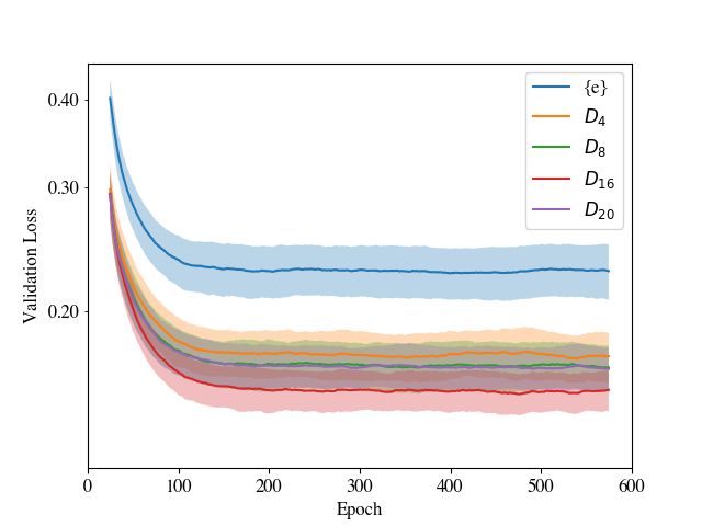
 Validation loss curves for both the standard CNN implementation,
 Fully-connected 120
 denoted { }, and the group-equivariant CNN implementations for
 ReLU
 Fully-connected 84 = {4, 8, 16, 20} are shown in Figure 2. Curves show the mean and
 ReLU standard deviation for each network over five training repeats. It can
 Dropout ( = 0.5) seen from Figure 2 that the standard CNN implementation achieves
 Fully-connected 2 a significantly poorer loss than that of its group-equivariant equiva-
 lents. For both the cyclic and dihedral group-equivariant models, the
 best validation loss is achieved for = 16. Although the final loss in
4 ARCHITECTURE the case of the cyclic and dihedral-equivariant networks is not sig-
 nificantly different in value, it is notable that the lower order dihedral
For our architecture we use a simple LeNet-style network (LeCun
 networks converge towards this value more rapidly than the equiv-
et al. 1998) with two convolutional layers, followed by three fully-
 alent order cyclic networks. We observe that higher order groups
connected layers. Each of the convolutional layers has a ReLU ac-
 minimize the validation loss more rapidly, i.e. the initial gradient of
tivation function and is followed by a max-pooling operation. The
 the loss as a function of epoch is steeper, up to order = 16 in this
fully-connected layers are followed by ReLU activation functions
 case. Weiler & Cesa (2019), who also noted the same thing when
and we use a 50% dropout before the final fully-connected layer, as
 training on the MNIST datasets, attribute this behaviour to the in-
is standard for LeNet (Krizhevsky et al. 2012). An overview of the
 creased generalisation capacity of equivariant networks, since there
architecture is shown in Table 4. In what follows we refer to this base
 is no significant difference in the number of learnable parameters
architecture using conventional convolution layers as the standard
 between models.
CNN and denote it { }. We also note that the use of conventional
 Final validation error as a function of order, , for the group-
CNN is used through the paper to refer to networks that do not employ
 equivariant networks is shown in Figure 3. From this figure it can be
group-equivariant convolutions, independent of architecture.
 seen that all equivariant models improve upon the non-equivariant
 For the -steerable implementation of this network we use the
 CNN baseline, { }, and that the validation error decreases before
e2cnn extension2 to the PyTorch library (Weiler & Cesa 2019)
 reaching a minimum for both cyclic and dihedral models at ap-
and replace the convolutional layers with their subgroup-equivariant
 proximately 16 orientations. This behaviour is discussed further in
equivalent. We also introduce two additional steps into the network
 Section 6.4.
in order to recast the feature data from the convolutional layers into
a format suitable for the conventional fully-connected layers. These
steps consist of reprojecting the feature data from a geometric tensor 5.2 Performance of G-Steerable CNNs
into standard tensor format and pooling over the group features, and
are indicated in italics in Table 4. Since the additional steps in the Standard performance metrics for both the standard CNN implemen-
 -steerable implementations have no learnable parameters associ- tation, denoted { }, and the group-equivariant CNN implementations
ated with them, the overall architecture is unchanged from that of the for = {4, 8, 16, 20} are shown in Table 5. The metrics in this table
standard CNN; it is only the nature of the kernels in the convolutional are evaluated using the reserved test set of the MiraBest∗ data set,
layers that differ. classified using the best-performing model according to the valida-
 For the input data we use the trivial representation, but for all tion early-stopping criterion. The reserved test set is augmented by a
subsequent steps in the -steerable implementations we adopt the factor of 9 using discrete rotations of 20◦ over the interval [0◦ , 180◦ ).
regular representation, reg . This representation is typical for de- This augmentation is performed in order to provide metrics that re-
scribing finite groups/subgroups such as and . The regular flect the performance over a consistent range of orientations. The
representation of a finite group acts on a vector space R | | by values in the table show the mean and standard deviation for each
permuting its axes, where | | = for and | | = 2 for , metric over five training repeats. All -steerable CNNs listed in this
 table use a regular representation for feature data and apply a -
 invariant map after the convolutional layers to guarantee an invariant
2 https://github.com/QUVA-Lab/e2cnn prediction.

 MNRAS 000, 1–11 (2015)

6 A. M. M. Scaife & F. Porter

Figure 2. Validation losses during the training of the standard CNN, denoted { }, and (i) -equivariant models for the MiraBest∗ data set (left), and (ii)
 -equivariant models for the MiraBest∗ data set (right). Plots show mean and standard deviation over five training repeats. Curves are smoothed over 20
epochs to eliminate small-scale variability.

Table 5. Performance metrics for classification of the MiraBest∗ data set using the standard CNN ({ }) and -steerable CNNs for different cyclic and dihedral
subgroups of the E(2) Euclidean group. All -steerable CNNs use a regular representation for feature data and apply a G-invariant map after the convolutions
to guarantee an invariant prediction.

 FRI FRII
 MiraBest∗ Accuracy [%] Precision Recall F1-score Precision Recall F1-score

 { } 94.04 ± 1.37 0.935 ± 0.018 0.940 ± 0.024 0.937 ± 0.015 0.946 ± 0.020 0.941 ± 0.018 0.944 ± 0.013

 4 95.24 ± 1.23 0.942 ± 0.018 0.959 ± 0.015 0.950 ± 0.013 0.963 ± 0.013 0.947 ± 0.018 0.955 ± 0.012
 8 95.96 ± 1.06 0.950 ± 0.020 0.966 ± 0.016 0.958 ± 0.011 0.969 ± 0.013 0.954 ± 0.019 0.961 ± 0.010
 16 96.07 ± 1.03 0.953 ± 0.020 0.964 ± 0.013 0.959 ± 0.011 0.968 ± 0.011 0.958 ± 0.019 0.963 ± 0.010
 20 95.88 ± 1.12 0.951 ± 0.019 0.962 ± 0.013 0.957 ± 0.012 0.966 ± 0.011 0.956 ± 0.018 0.961 ± 0.011

 4 95.45 ± 1.38 0.948 ± 0.024 0.957 ± 0.017 0.952 ± 0.014 0.962 ± 0.015 0.952 ± 0.023 0.957 ± 0.013
 8 96.37 ± 0.95 0.960 ± 0.019 0.964 ± 0.014 0.962 ± 0.010 0.968 ± 0.012 0.964 ± 0.018 0.966 ± 0.009
 16 96.56 ± 1.29 0.963 ± 0.025 0.965 ± 0.014 0.964 ± 0.013 0.969 ± 0.012 0.966 ± 0.023 0.967 ± 0.012
 20 96.39 ± 1.00 0.959 ± 0.018 0.966 ± 0.015 0.962 ± 0.010 0.969 ± 0.013 0.962 ± 0.017 0.966 ± 0.010

 From Table 5, it can be seen that the best test accuracy is achieved
 by the 16 model, highlighted in bold. Indeed, while all equivariant
 models perform better than the standard CNN, the performance of
 the dihedral models is consistently better than for the cyclic models
 of equivalent order.
 For the cyclic models it can be observed that the largest change
 in performance comes from an increased FRI recall. For a binary
 classification problem, the recall of a class is defined as
 TP
 Recall = , (5)
 TP + FN
 where TP indicates the number of true positives and FN indicates the
 number of false negatives. The recall therefore represents the fraction
 of all objects in that class which are correctly classified. Equivalently,
 the precision of the class is defined as
 TP
 Precision = . (6)
 TP + FP
Figure 3. Validation errors of and regular steerable CNNs for Consequently, if the recall of one class increases at the expense of
different orders, , for the MiraBest∗ data set. All equivariant models improve the precision of the opposing class then it indicates that the opposing
upon the non-equivariant CNN baseline, { }. class is being disproportionately misclassified. However, in this case
 we can observe from Table 5 that the precision of the FRII class is also

MNRAS 000, 1–11 (2015)

E(2)-equivariant radio galaxy classification 7
 test sample. This posterior distribution allows one to assess the de-
 gree of certainty with which a prediction is being made, i.e. if the
 distribution of outputs for a particular class is well-separated from
 those of other classes then the input is being classified with high
 confidence; however, if the distribution of outputs intersects those
 of other classes then, even though the softmax probability for a par-
 ticular realisation may be high (even as high as unity), the overall
 distribution of softmax probabilities for that class may still fill the
 entire [0, 1] range, overlapping significantly with the distributions
 from other target classes. Such a circumstance denotes a low degree
 of model certainty in the softmax probability and therefore in the
 class prediction for that particular test sample.
 By re-enabling the dropout before the final fully-connected layer
 at test time, we estimate the predictive uncertainty of each model
 for the data samples in the reserved MiraBest∗ test set. With dropout
 enabled, we perform = 50 forward passes through the trained
 network for each sample in the test set. On each pass we recover
 ( , ), where and are the softmax probabilities of FRI and
 FRII, respectively. An example of the results from this process can
Figure 4. Average number of misclassifications for FRI (cyan) and FRII (grey) be seen in Figure 5, where we evaluate the trained model on a rotated
over all orientations and training repeats for the standard CNN, denoted { }, version of the input image at discrete intervals of 20◦ in the range
the 16 CNN and the 16 CNN, see Section 5.2 for details. [0◦ , 180◦ ) using a trained model for the standard CNN (left panel)
 and for the 16 -equivariant CNN (right panel). For each rotation
 angle, a distribution of softmax probabilities is obtained. In the case
increasing, suggesting that the improvement in performance is due to of the standard CNN it can be seen that, although the model classifies
a smaller number of FRI objects being misclassified as FRII. For the the source with high confidence when it is unrotated (0◦ ), the soft-
cyclic models there is a smaller but not equivalent improvement in max probability distributions are not well-separated for the central
FRII recall. This suggests that the cyclic model primarily reduces the image orientations, indicating that the model has a lower degree of
misclassification of FRI objects as FRII, but does not equivalently confidence in the prediction being made in at these orientations. For
reduce the misclassification of FRII as FRI. the 16 -equivariant CNN it can be seen that in this particular test
 The dihedral models show a more even distribution of improve- case the model has a high degree of confidence in its prediction for
ment across all metrics, indicating that there are more balanced reduc- all orientations of the image.
tions across both FRI and FRII misclassifications. This is illustrated To represent the degree of uncertainty for each test sample quanti-
in Figure 4, which shows the average number of misclassifications tatively, we evaluate the degree of overlap in the distributions of soft-
over all orientations and training repeats for the standard CNN, the max probabilities at a particular rotation angle using the distribution-
 16 CNN and the 16 CNN for the reserved test set. free overlap index (Pastore & Calcagnì 2019). To do this, we calculate
 The test partition of the full Mirabest data set contains 153 FRI the local densities at position for each class using a Gaussian kernel
and FRII-type sources labelled as both Confident and Uncertain, see density estimator, such that
Table 3. When using this combined test set the overall performance
 
metrics of the networks considered in this work become accordingly 1 ∑︁ 1 2 2
lower due to the inclusion of the Uncertain sources. This is expected, ( ) = √ e−( − ) /2 , (7)
 
 =1 2 
not only because the Uncertain samples include edge cases that are
 
more difficult to classify but also because the assigned labels for these 1 ∑︁ 1 2 2
objects may not be fully accurate. However, the relative performance ( ) = √ e−( − ) /2 , (8)
 =1 2 
 
shows the same degree of improvement between the standard CNN,
{ }, and the 16 model, which have percentage accuracies of 82.59± where = 0.1. We then use these local densities to calculate the
1.41 and 85.30 ± 1.35, respectively, when evaluated against this overlap index, , such that
combined test set. 
 ∑︁
 We note that given the comparatively small size of the Mirabest∗
  
 = min ( ), ( ) , (9)
training set, these results may not generalise equivalently to other =1
potentially larger data sets with different selection specifications and 
 where { } =1 covers the range zero to one in steps of size .
that additional validation should be performed when considering
 For this work we assume = 100. The resulting overlap index, ,
the use of group-equivariant convolutions for other classification
 varies between zero and one, with larger values indicating a higher
problems.
 degree of overlap and hence a lower degree of confidence.
 For each test sample we evaluate the overlap index over a range of
 rotations from 0◦ to 180◦ in increments of 20◦ . We then calculate the
5.3 On the confidence of G-Steerable CNNs
 average overlap index, h i, across these nine rotations. In Figure 5
Target class predictions for each test data sample are made by se- the value of this index can be seen above each plot: in this case, the
lecting the highest softmax probability, which provides a normalised standard CNN has h i { } = 0.30 and the 16 -equivariant CNN has
version of the network output values. By using dropout as a Bayesian h i 16 < 0.01.
approximation, as demonstrated in Gal & Ghahramani (2015), one Of the 104 data samples in the reserved test set, 27.7 ± 11.0%
is able to obtain a posterior distribution of network outputs for each of objects show an improvement in average model confidence, i.e.

 MNRAS 000, 1–11 (2015)

8 A. M. M. Scaife & F. Porter

Figure 5. A scatter of 50 forward passes of the softmax output for the standard CNN (left) and the 16 -equivariant CNN (right). The lower panel shows the
rotated image of the test image. As indicated, the average overlap index for the standard CNN is h i = 0.30, and h i < 0.01 for the 16 -equivariant CNN.

h i { } − h i 16 > 0.01, when classified using the 16 -equivariant et al. 2015). The observational evidence for both remains a subject
CNN compared to the standard CNN, 8.4±2.5% show a deterioration of discussion in the literature.
in average model confidence, i.e. h i 16 −h i { } > 0.01, and all other Taylor & Jagannathan (2016) found a local alignment of radio
samples show no significant change in average model confidence, galaxies in the ELAIS N1 field on scales < 1◦ using observations
i.e. |h i { } − h i 16 | < 0.01. Mean values and uncertainties are from the Giant Metrewave Radio Telescope (GMRT) at 610 MHz.
determined from h i values for all test samples evaluated using a Local alignments were also reported by Contigiani et al. (2017) who
pairwise comparison of 5 training realisations of the standard CNN reported evidence (> 2 ) of local alignment on scales of ∼ 2.5◦
and 5 training realisations of the 16 CNN. among radio sources from the FIRST survey using a much larger
 Those objects that show an improvement in average model confi- sample of radio galaxies, catalogued by the radio galaxy zoo project.
dence are approximately evenly divided between FRI and FRII type A similar local alignment was also reported by Panwar et al. (2020)
objects, whereas the objects that show a reduction in model confi- using data from the FIRST survey. Using a sample of 7555 double-
dence exhibit a weak preference for FRII. These results are discussed lobed radio galaxies from the LOFAR Sky Survey (LoTSS; Shimwell
further in Section 6.1. et al. 2019) at 150 MHz, Osinga et al. (2020) concluded that a statis-
 tical deviation from purely random distributions of orientation as a
 function of projected distance was caused by systematics introduced
 by the brightest objects and did not persist when redshift information
6 DISCUSSION was taken into account. However, the study also suggested that larger
 samples of radio galaxies should be used to confirm this result.
6.1 Statistical distribution of radio galaxy orientations
 Whilst these results may suggest tentative evidence for spatial cor-
Mathematically, -steerable CNNs classify equivalence classes of relations of radio galaxy orientations in local large-scale structure,
images, as defined by the equivalence relation of a particular group, they do not provide any information on whether these orientations
 , whereas conventional CNNs classify equivalence classes defined differ between classes of radio galaxy, i.e. the equivalence classes
only by translations. Consequently, by using E(2)-equivalent convo- considered here. Moreover, the large spatial distribution and com-
lutions the trained models assume that the statistics of extra-galactic paratively small number of galaxies that form the training set used in
astronomical images containing individual objects are expected to this work mean that even spatial correlation effects would be unlikely
be invariant not only to translations but also to global rotations and to be significant for the data set used here. However, the results of
reflections. Here we briefly review the literature in order to consider Taylor & Jagannathan (2016); Contigiani et al. (2017); Panwar et al.
whether this assumption is robust and highlight the limitations that (2020) suggest that care should be taken in this assumption if data
may result from it. sets are compiled from only small spatial regions.
 The orientation of radio galaxies, as defined by the direction of In Section 5.1, we found that the largest improvement in perfor-
their jets, is thought to be determined by the angular momentum axis mance was seen when using dihedral, , models. We suggest that
of the super-massive black hole within the host galaxy. A number of this improvement over cyclic, , models is due to image reflections
studies have looked for evidence of preferred jet alignment directions accounting for chirality, in addition to orientations on the celestial
in populations of radio galaxies, as this has been proposed to be a sphere which are represented by the cyclic group. Galactic chirality
potential consequence of angular momentum transfer during galaxy has previously been considered for populations of star-forming, or
formation (e.g. White 1984; Codis et al. 2018; Kraljic et al. 2020), or normal, galaxies (see e.g. Slosar et al. 2009; Shamir 2020), as the
alternatively it could be caused by large-scale filamentary structures spiral structure of star-forming galaxies means that such objects can
in the cosmic web giving rise to preferential merger directions (see be considered to be enantiomers, i.e. their mirror images are not su-
e.g. Kartaltepe et al. 2008) that might result in jet alignment for radio perimposable (Capozziello & Lattanzi 2005). It has been suggested
galaxies formed during mergers (e.g. Croton et al. 2006; Chiaberge that a small asymmetry exists in the number of clockwise versus

MNRAS 000, 1–11 (2015)

E(2)-equivariant radio galaxy classification 9
anti-clockwise star-forming galaxy spins (Shamir 2020). As far as works aim to separate the orientation (typically referred to as the
the authors are aware there have been no similar studies considering viewpoint or pose in the context of capsule networks) of an object
the chirality of radio galaxies. However, a simple example of such from its nature, i.e. class, by encoding the output of their layers as tu-
chirality for radio galaxies might include the case where relativistic ples incorporating both a pose vector and an activation. The purpose
boosting causes one jet of a radio galaxy to appear brighter than the of this approach is to focus on the linear hierarchical relationships in
other due to an inclination relative to the line of sight. Since the dom- the data and remove sensitivity to orientation; however, as described
inance of a particular orientation relative to the line of sight should be by Lenssen et al. (2018), general capsule networks do not guaran-
unbiased then this would imply a global equivariance to reflection. tee particular group equivariances and therefore cannot completely
Since the dihedral ( ) models used in this work are insensitive disentangle orientation from feature data. It is perhaps partly for this
to chirality, the results in Section 5.1 suggest that the radio galaxies reason that Lukic et al. (2018) found that capsule networks offered
in the training sample used here do not have a significant degree of no significant advantage over standard CNNs for the radio galaxy
preferred chirality. Whilst this does not itself validate the assumption classification problem addressed in that work.
of global reflection invariance, in the absence of evidence to the con- In Section 5, we found that not only is the test performance im-
trary from the literature we suggest that it is unlikely to be significant proved by the use of equivariant CNNs, but that equivariant networks
for the data sample used in this work. also converge more rapidly. For image data, a standard CNN enables
 From the perspective of classification, equivariance to reflections generalization over classes of translated images, which provides an
implies that inference should be independent of reflections of the advantage over the use of an MLP, where every image must be consid-
input. For FR I and FR II radio galaxy classification, incorporating ered individually. -steerable CNNs extend this behaviour to include
such information into a classification scheme may be important more additional equivalences, further improving generalization. This ad-
generally: the unified picture of radio galaxies holds that both FR I and ditional equivariance enhances the data efficiency of the learning
FR II, as well as many other classifications of active galactic nuclei algorithm because it means that every image is no longer an indi-
(AGN) such as quasars, QSOs (quasi-stellar objects), blazars, BL vidual data point but instead a representative of its wider equiva-
Lac objects, Seyfert galaxies etc., are in fact defined by orientation- lence group. Consequently, unlike capsule networks, the equivalence
dependent observational differences, rather than intrinsic physical groups being classified by a -steerable CNN are specified a priori,
distinctions (Urry 2004). rather than the orientations of individual samples being learned dur-
 Consequently, under the assumptions of global rotational and re- ing training. Whilst this creates additional capacity in the network
flection invariance, the possibility of a classification model providing for learning intra-class differences that are insensitive to the specified
different output classifications for the same test sample at different equivalences, it does not provide the information on orientation of
orientations is problematic. Furthermore, the degree of model confi- individual samples that is provided as an output by capsule networks.
dence in a classification should also not vary significantly as a func- Lenssen et al. (2018) combined group-equivariant convolutions
tion of sample orientation, i.e. if a galaxy is confidently classified with capsule networks in order to output information on both classifi-
at one particular orientation then it should be approximately equally cation and pose, although they note that a limitation of this combined
confidently classified at all other orientations. If this is not the case, approach is that arbitrary pose information is no longer available, but
as shown for the standard CNN in Figure 5 (left), then it indicates a is instead limited to the elements of the equivariant group. For radio
preferred orientation in the model weights for a given outcome, in- astronomy, where radio galaxy orientations are expected to be ex-
consistent with the expected statistics of the true source population. tracted from images at a precision that is limited by the observational
Such inconsistencies might be expected to result in biased samples constraints of the data, it is unlikely that pose information limited
being extracted from survey data. to the elements of a low-order finite group, < (2), is sufficient
 In this context it is then not only the average degree of model for further analysis. However, given particular sets of observational
confidence that is important as a function of sample rotation, as and physical constraints or specifications it is possible that such an
quantified by the value of h i in Section 5.3, but also the stability approach may become useful at some limiting order. Alternatively,
of the index as a function of rotation, i.e. a particular test sample pose information might be used to specify a prior for a secondary
should be classified at a consistent degree of confidence as a function processing step that refines a measurement of orientation.
of orientation, whether that confidence is low or high. To evaluate
the stability of the predictive confidence as a function of orientation,
we examine the variance of the index as a function of rotation. For 6.3 Local vs Global Equivariance
the MiraBest∗ reserved test set we find that approximately 30% of By design, the final features used for classification in equivariant
the test samples show a reduction of more than 0.01 in the standard CNNs do not include any information about the global orientation
deviation of their overlap index as a function of rotation, with 17% or chirality of an input image; however, this can also mean that they
showing a reduction of more than 0.05. Conversely approximately are insensitive to local equivariances in the image, when these might
8% of test samples show an increase of > 0.01 and 4% samples show in fact be useful for classification. The hierarchical nature of con-
an increase of > 0.05. In a similar manner to the results for average volutional networks can be used to mitigate against this, as kernels
model confidence given in Section 5.3, those objects that show a corresponding to earlier layers in a network will have a smaller, more
reduction in their variance, i.e. an improvement in the consistency of local, footprint on the input image and therefore be sensitive to a
prediction as a function of rotation, are evenly balanced between the different scale of feature than those from deeper layers which en-
two classes; however, those objects showing a strong improvement compass larger-scale information. Therefore, by changing the degree
of > 0.05 are preferentially FRI type objects. of equivariance as a function of layer depth one can control the de-
 gree to which local equivariance is enforced. Weiler & Cesa (2019)
 refer to this practice as group restriction and find that it is beneficial
6.2 Comment on Capsule Networks
 when classifying data sets that possess symmetries on a local scale
The use of capsule networks (Sabour et al. 2017) for radio galaxy but not on a global scale, such as the CIFAR and unrotated MNIST
classification was investigated by Lukic et al. (2018). Capsule net- datasets. Conversely, the opposite situation may also be true, where

 MNRAS 000, 1–11 (2015)

10 A. M. M. Scaife & F. Porter
 7 CONCLUSIONS

 In this work, we have demonstrated that the use of even low-order
 group-equivariant convolutions results in a performance improve-
 ment over standard convolutions for the radio galaxy classification
 problem considered here, without additional hyper-parameter tun-
 ing. We have shown that both cyclic and dihedral equivariant models
 converge to lower validation loss values during training and provide
 improved validation errors. We attribute this improvement to the in-
 creased capacity of the equivariant networks for learning hierarchical
 features specific to classification, when additional capacity for en-
 coding redundant feature information at multiple orientations is no
 longer required, hence reducing intra-class variability.
 We have shown that for the simple network architecture and train-
 ing set considered here, a 16 equivariant model results in the best
 test performance using a reserved test set. We suggest that the im-
 provement of the dihedral over the cyclic models is due to an in-
 sensitivity to - and therefore lack of preferred - chirality in the data,
Figure 6. Validation losses during the training of the standard CNN, denoted
 and that further improvements in performance might be gained from
{ } (blue), the 16 CNN (orange), and the restricted | 1 { } CNN (green;
 tuning the size of the kernels in the convolutional layers according to
dashed) for the MiraBest∗ data set. Plots show mean and standard deviation
over five training repeats. the order of the equivalence group. We find that cyclic models pre-
 dominantly reduce the misclassification of FRI type radio galaxies,
 whereas dihedral models reduce misclassifications for both FRI and
no symmetry is present on a local scale, but the data are statistically FRII type galaxies.
invariant on a global scale. In this case the reverse may be done and, By using the MC Dropout Bayesian approximation method, we
rather than restricting the representation of the feature data to re- have shown that the improved performance observed for the 16
duce the degree of equivariance, one might expand the domain of the model compared to the standard CNN is reflected in the model con-
representation at a particular layer depth in order to reflect a global fidence as a function of rotation. Using the reserved test set, we have
equivariance. quantified this difference in confidence using the overlap between
 We investigate the effect of group restriction by using a | 1 { } predictive probability distributions of different target classes, as en-
restricted version of the LeNet architecture, i.e. the first layer is capsulated in the distribution free overlap index parameter, . We
equivariant and the second convolutional layer is a standard convo- find that not only is average model confidence improved when using
lution. Using = 16, the loss curve for this restricted architecture the equivariant model, but also that the consistency of model confi-
relative to the unrestricted 16 equivariant CNN is shown in Fig- dence as a function of image orientation is improved. We emphasise
ure 6. From the figure it can be seen that while exploiting local the importance of such consistency for applications of CNN-based
symmetries gives an improved performance over the standard CNN, classification in order to avoid biases in samples being extracted from
the performance of the group restricted model is significantly poorer future survey data.
than that of the full 16 CNN. This result suggests that although
 Whilst the results presented here are encouraging, we note that this
local symmetries are present in the data, it is the global symmetries
 work addresses a specific classification problem in radio astronomy
of the population that result in the larger performance gain for the
 and the method used here may not result in equivalent improvements
radio galaxy data set.
 when applied to other areas of astronomical image classification us-
 ing different data sets or network architectures. In particular, the as-
 sumptions of global rotational and reflectional invariance are strong
6.4 Note on hyper-parameter tuning
 assumptions, which may not apply to all data sets. As described in
In Section 5 we found that the = 16 cyclic and dihedral models Section 6.1, data sets extracted from localised regions of the sky
were preferred over the higher order = 20 models. This may may be particularly vulnerable to biases when using this method and
seem counter-intuitive as one might assume that for truly rotationally the properties of the MiraBest∗ data set used in this work may not
invariant data sets the performance would converge to a limiting generalise to all other data sets or classification problems. We note
value as the order increased, rather than finding a minimum at some that this is true for all CNNs benchmarked against finite data sets and
discrete point. Consequently, we note that the observed minimum at users should be aware that additional validation should be performed
 = 16 might not represent a true property of the data set but instead before models are deployed on new test data, as biases arising from
represent a limitation caused by discretisation artifacts from rotation data selection may be reflected in biases in classifier performance
of convolution kernels with small support, in this case = 5, see (see e.g. Wu et al. 2018; Tang 2019; Walmsley et al. 2020). However,
Table 4 (Weiler & Cesa 2019). These same discretisation errors may in conclusion, we echo the expectation of Weiler & Cesa (2019),
also account in part for the small oscillation in validation error as that equivariant CNNs may soon become a common choice for mor-
a function of group order seen in Figure 3. Consequently, while no phological classification in fields like astronomy, where symmetries
additional hyper-parameter tuning has been performed for any of the may be present in the data, and note that the overhead in constructing
networks used in this work, we note that kernel size is potentially such networks is now minimal due to the emergence of standardised
one hyper-parameter that could be tuned as a function of group libraries such as e2cnn. Future work will need to address the op-
order, , and that such tuning might lead to further improvements in timal architectures and hyper-parameter choices for such models as
performance for higher orders. specific applications evolve.

MNRAS 000, 1–11 (2015)