Prediction of Yield Productivity Zones from Landsat 8 and Sentinel-2A/B and Their Evaluation Using Farm Machinery Measurements - MDPI
←
→
Page content transcription
If your browser does not render page correctly, please read the page content below
remote sensing
Article
Prediction of Yield Productivity Zones from Landsat 8
and Sentinel-2A/B and Their Evaluation Using Farm
Machinery Measurements
Tomáš Řezník 1, *, Tomáš Pavelka 1 , Lukáš Herman 1 , Vojtěch Lukas 2 , Petr Širůček 2 ,
Šimon Leitgeb 1 and Filip Leitner 1
 1    Department of Geography, Faculty of Science, Masaryk University, Kotlářská 2, 611 37 Brno, Czech Republic;
      pavelka.tomas@mail.muni.cz (T.P.); herman.lu@mail.muni.cz (L.H.); leitgeb@mail.muni.cz (Š.L.);
      451242@mail.muni.cz (F.L.)
 2    Department of Agrosystems and Bioclimatology, Faculty of Agronomy, Mendel University, Zemědělská 1,
      613 00 Brno, Czech Republic; vojtech.lukas@mendelu.cz (V.L.); qqsiruce@node.mendelu.cz (P.Š.)
 *    Correspondence: tomas.reznik@sci.muni.cz; Tel.: +42-0549-49-4460

 Received: 14 May 2020; Accepted: 11 June 2020; Published: 13 June 2020

 Abstract: Yield is one of the primary concerns for any farmer since it is a key to economic prosperity.
 Yield productivity zones—that is to say, areas with the same yield level within fields over the
 long-term—are a form of derived (predicted) data from periodic remote sensing, in this study
 according to the Enhanced Vegetation Index (EVI). The delineation of yield productivity zones can
 (a) increase economic prosperity and (b) reduce the environmental burden by employing site-specific
 crop management practices which implement advanced geospatial technologies that respect soil
 heterogeneity. This paper presents yield productivity zone identification and computing based on
 Sentinel-2A/B and Landsat 8 multispectral satellite data and also quantifies the success rate of yield
 prediction in comparison to the measured yield data. Yield data on spring barley, winter wheat, corn,
 and oilseed rape were measured with a spatial resolution of up to several meters directly by a CASE
 IH harvester in the field. The yield data were available from three plots in three years on the Rostěnice
 Farm in the Czech Republic, with an overall acreage of 176 hectares. The presented yield productivity
 zones concept was found to be credible for the prediction of yield, including its geospatial variations.

 Keywords: yield productivity zones; yield measurements; satellite images; precision agriculture;
 Enhanced Vegetation Index

1. Introduction
     Estimating potential crop yield is a crucial activity performed in the assessment of seasonal
production. It has been well established by works such as Auernhammer [1] that a plot is not a
homogeneous area from the point of view of soil conditions, climate, or crop yield. The period of the
past 20 years may be characterized as a shift from conventional farming to precision farming. Precision
farming techniques count and rely on such heterogeneity. All plots have their strong as well as weak
zones from the crop yield point of view.
     Information on yield is important for two main reasons: it can be used (a) to maximize economic
profitability and (b) to reduce the environmental burden caused by agricultural activities. Both objectives
require as much accurate information on the yield as possible. However, according to the results of
several European research projects [2,3] in particular, detailed geospatial data on yield with a spatial
resolution of a few meters are scarce, since information on yield is typically available only for larger
aggregated areas—i.e., plot level, farm level, and/or regional level [4]. Therefore, indirect methods for
yield prediction have therefore been developed and verified. Such indirect methods aim at estimations

Remote Sens. 2020, 12, 1917; doi:10.3390/rs12121917                          www.mdpi.com/journal/remotesensing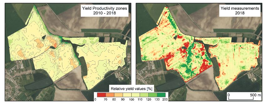
Remote Sens. 2020, 12, 1917 2 of 17
of yield, typically for a certain crop, area, and time. Their common approach is to analyze climatic
as well as soil conditions, agronomic practices, and crop growth characteristics [5–7]. Such methods
aim at identifying crop yield potential, which is defined as the maximum attainable yield per unit
land area that can be achieved under non-limited nutrient application and the full control of pests,
diseases, weeds, lodging, and other stress factors [8,9]). The difference between the estimated yield
from the identified productivity zone and the farm yield is determined as the yield gap [10]. Examples
of methods for estimating the yield from the productivity zone and yield gaps may be found in
Van Wart et al. [11], Van Ittersum et al. [12], and Chen et al. [13].
In contrast, universal indirect methods are also being elaborated on for the assessment of actual
crop growth and yield based on remote sensing [14–16]. Their main motivation is to establish a model
based on vegetative indices that is capable of identifying highly productive and less productive zones
within a plot and linking these to the actual or potential crop yield. Recent studies have described
the adaption of remotely sensed crop properties as indicators of the yield level and yield forecast
for given soil/climate conditions and crop management practices using data mainly from satellite
sensors, such as AVHRR [17], MODIS [18–20], or Sentinel-2 [21]. However, the identification of crop
productivity within fields in precision agriculture is, in most cases, focused on the spatial delineation of
zones rather than on the precise forecast of attainable crop yields. For these reasons, data with a higher
spatial resolution are needed, as shown by Thenkabail [22] or Gu and Wylie [23]. Therefore, the use of
yield productivity zones is an input for decision-making at the farm level which does not exclude the
need for analyzing the climate, soils, and agronomic practices, etc. Nevertheless, productivity zones
are a universal model that may be applied to similar crops (such as wheat, barley, and corn) and areas
with similar climatic and soil conditions.
This paper aims at the discovery and verification of long-term high and low yield productivity
zones, as they are areas where crop yield has been for several years significantly above or below
the average yield for the whole plot and because they require the site-specific tailoring of fertilizer
application rates to ensure the most efficient use of nutrients for the determined level of yield production.
In addition, the identification of such zones can help to minimize environmental pollution by the
residues of agrochemical substances (fertilizers, pesticides) [24]. Addressing within-field spatial
variability by delineating yield productivity zones is crucial for site-specific crop management in
precision agriculture [25,26] and follows the concept of sustainable food production (Bongiovanni and
Lowenberg-Deboer [27], as well as Gebbers and Adamchuk [28]). The term “long-term” in this context
means for as long as agronomical practices do not change significantly—that is to say, for as long as they
remain comparable. The motivations to discover high/low crop yield productivity zones are therefore
economic and environmental—increasing profitability by saving on fertilizer, fuel, and manpower on
the one hand and avoiding the overuse of agrochemicals on the other in order to reduce the soil and/or
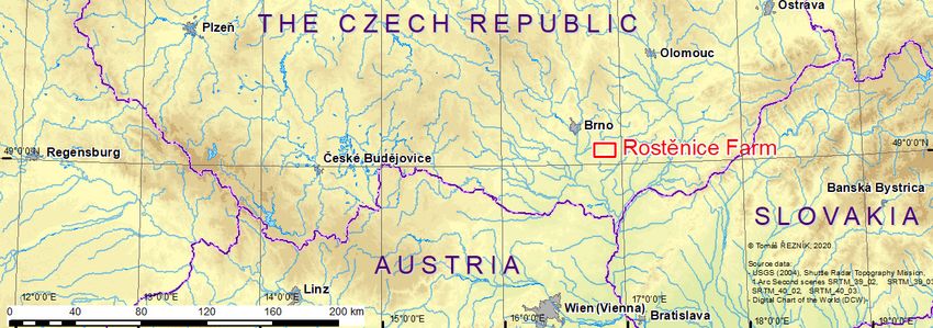
water pollution [29,30]. This research was verified at Rostěnice Farm in the Czech Republic, whose
geographical location is depicted in Figure 1 and whose agronomical characteristics are documented in
Section 2.1.
The above-mentioned requirements for the identification of long-term below-average and
above-average areas with respect to yield, meaning yield productivity zones, come from farmers as
well as other stakeholders. For instance, the discovery of long-term high/low yield productivity zones
was also a goal of the Global Earth Observation System of Systems (GEOSS) AIP-8 (Global Earth
Observation System of Systems’ Architecture Implementation Pilot 8) targeting agricultural and water
pollution [31]. Agriculture and water pollution is therefore the subject of (inter)national legislation,
such as the Clean Water Act in the United States of America [32], the European Water Framework
Directive [23–35], and the Law of the People’s Republic of China on the Prevention and Control of
Water Pollution [36]. The following text presents research results concerning the identification of
long-term high/low yield productivity zones for cereals conducted within the GEOSS as well as within
three European Union-funded research projects, namely the FOODIE (Farm-Oriented Open Data in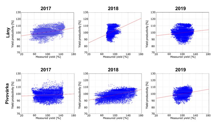
beyond the scope of this paper. Long-term high/low yield productivity zones should be understood
as one kind of information input for further modelling and/or decision-making, not as a general
approach or solution to the problem of yield prediction.
      The primary goal of this paper is to present means of yield productivity zone identification and
computing
Remote         based
       Sens. 2020,      on the Sentinel-2A/B and Landsat 8 multispectral satellite data. An eight-year series
                   12, 1917                                                                            3 of 17
(2013–2019) from Sentinel-2A/B and Landsat 8 missions was used for the prediction of yield
productivity zones. The secondary goal of this paper is to provide quantitative verifications. A four-
Europe [37]), DataBio (Data-Driven Bioeconomy [38,39]), and SIEUSOIL (Sino-EU Soil Observatory for
year series (2016–2019) of in situ sensor measurements from the CASE IH harvester in three plots was
intelligent Land Use Management [40]) projects.
used as reference data for this evaluation.

                              Figure 1.
                              Figure 1. Geographical location of
                                        Geographical location of the
                                                                 the Rostěnice
                                                                     Rostěnice Farm.
                                                                                Farm.

2. Materials
     It shouldand    Methods
                 be noted   that how such computed long-term high/low yield productivity zones are used
in decision-making      processes
      Methods of periodic satellite  related   to farm
                                          remote         practice—e.g.,
                                                   sensing   were used fortheyield
                                                                              application  of fertilizers—is
                                                                                   productivity               beyond
                                                                                                  zone identification
the
andscope    of this since
     computing,      paper.neither
                             Long-term      high/low
                                      operative    aerialyield productivity
                                                           remote  sensing norzones  should be understood
                                                                                  meteorological    monitoringaswere
                                                                                                                   one
kind  of information     input for  further   modelling
available for Rostěnice Farm in the Czech Republic.        and/or  decision-making,    not as a general   approach   or
solution to the problem of yield prediction.
     The primaryCharacteristics
2.1. Agronomical      goal of this paper
                                      of the is to present
                                             Pilot  Farm means of yield productivity zone identification and
computing based on the Sentinel-2A/B and Landsat 8 multispectral satellite data. An eight-year series
      The farm
(2013–2019)   fromdata    on the yield
                     Sentinel-2A/B    and measurements
                                           Landsat 8 missions were
                                                                 was provided    by prediction
                                                                      used for the  Rostěnice ofFarm
                                                                                                   yieldinproductivity
                                                                                                            the Czech
Republic
zones.     (Figure
         The         1). Data
              secondary        onof
                            goal  thethis
                                        crops,
                                           paper agronomic    practices,
                                                    is to provide        and yield
                                                                   quantitative     measurements
                                                                                  verifications.      (see Section
                                                                                                  A four-year      2.3)
                                                                                                                 series
were   provided    for the  purposes    of this   paper.
(2016–2019) of in situ sensor measurements from the CASE IH harvester in three plots was used as
      The farm,
reference  data forRostěnice   a.s. (N49.105 E16.882), manages over 10,000 ha of arable land in the South
                      this evaluation.
Moravia region of the Czech Republic. The average annual rainfall is 544 mm, and the average annual
temperature
2. Materials andis 8.8°C.  Within the managed land, the prevalence of soil type is Chernozem, Cambisol,
                     Methods
haplic Luvisol, Fluvisol near to water bodies, and occasionally also Calcic Leptosols. The main
     Methods of periodic satellite remote sensing were used for yield productivity zone identification
program is plant production, where the main focus is on the cultivation of malting barley (2500 ha),
and computing, since neither operative aerial remote sensing nor meteorological monitoring were
maize for grain and biogas production (2500 ha), winter wheat (2000 ha), oilseed rape (1000 ha), and
available for Rostěnice Farm in the Czech Republic.

2.1. Agronomical Characteristics of the Pilot Farm
     The farm data on the yield measurements were provided by Rostěnice Farm in the Czech Republic
(Figure 1). Data on the crops, agronomic practices, and yield measurements (see Section 2.3) were
provided for the purposes of this paper.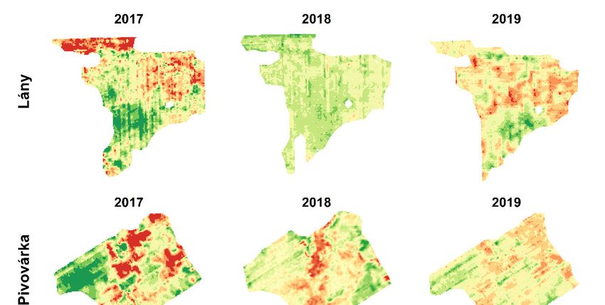
Remote Sens. 2020, 12, 1917                                                                                  4 of 17

      The farm, Rostěnice a.s. (N49.105 E16.882), manages over 10,000 ha of arable land in the South
Moravia region of the Czech Republic. The average annual rainfall is 544 mm, and the average annual
temperature is 8.8 ◦ C. Within the managed land, the prevalence of soil type is Chernozem, Cambisol,
haplic Luvisol, Fluvisol near to water bodies, and occasionally also Calcic Leptosols. The main program
is plant production, where the main focus is on the cultivation of malting barley (2500 ha), maize for
grain and biogas production (2500 ha), winter wheat (2000 ha), oilseed rape (1000 ha), and other crops
and products such as soybean and lamb. The average production intensity is 6 t/ha for malting barley,
7 t/ha for winter wheat, 10 t/ha for grain maize, and 4 t/ha for oilseed rape. The farm has applied
long-term soilless cultivation (mostly choppers) on their land, leaving all straw after harvest on the
land. The high spatial variability of soil conditions in the southern part of farm has led to the adoption
of precision farming practices, such as the variable application of fertilizers (since 2006) and crop
yield mapping by harvesters. This farm manages over 10,000 ha under minimum soil tillage practices,
including an area with a variable rate application of mineral fertilizers. The main crops are winter
wheat, spring barley, oilseed rape, and maize.
      Table 1 shows the list of crops that were cultivated in the study area from 2013 to 2019—i.e., the time
period for which the yield productivity zones were computed (2013–2019) and the years in which the
yield was measured directly in the plots (2016–2019).

      Table 1. Information on crops from 2013 to 2019 for the area of study for which the yield productivity
      zones were computed. The years in which the yield measurements from the field harvesters were
      available are highlighted with a grey background.

  Year    “Lány” Plot (ID 2401/20)        “Pivovárka” Plot (ID 2401/9)    “Přední Prostřední” Plot (ID 2401/12)
  2013           spring barley                    spring barley                       maize (corn)
  2014           winter wheat                     maize (corn)                        spring barley
  2015            oilseed rape                    maize (corn)                        maize (corn)
  2016           winter wheat                     spring barley                       maize (corn)
  2017           winter wheat                     spring barley                       maize (corn)
  2018            oilseed rape                    maize (corn)                        spring barley
  2019           winter wheat                     spring barley                       spring barley

2.2. Yield Productivity Zone Identification and Computation
     The conducted study comprised the following methodological steps. Multispectral satellite
images were used as the primary source of information for yield productivity zone identification,
while yield measurements for three plots at Rostěnice Farm from 2016 to 2019 were used as reference
data (see Section 2.1). An eight-year series (2013–2019) was composed from Landsat 8 as well as
Sentinel-2A/B [41] imagery, as depicted in the Supplementary Material 1. The yield productivity zones
were computed from this eight-year series of satellite data according to the Enhanced Vegetation Index
(EVI) as defined through the following equation, Equation (1).

                              EVI = [2.5 × (NIR - Red)/(NIR + 6 × Red - 7.5 × Blue + 1)],                       (1)

 where:
     EVI: Enhanced Vegetation Index,
     NIR: near-infrared (band).
     Huete et al. [42,43], as well as Johnson et al. [44] have shown EVI to exhibit higher sensitivities to
crop parameters than the more commonly used NDVI (Normalized Difference Vegetation Index). For
each plot, the median and quantile values of yield productivity were computed separately. The yield
productivity zones (prediction) were then correlated with yield measurements for three plots in three
years, meaning the plots for which actual yield measurements were available (see Section 2.3). Besides
the statistical verification, qualitative research was also conducted for farms that do not have yield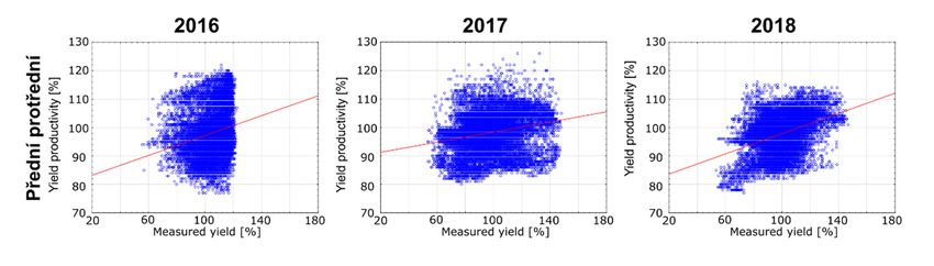
Remote Sens. 2020, 12, 1917                                                                          5 of 17

measurements in the form of a map. A dozen farms from seven countries compared their knowledge
on yield with yield productivity zone maps and shared their results.
      The concept of yield productivity zones, in contrast to yield crop potential, aims at establishing a
more universal model that may be re-used for other crops—in this study, for cereals in a temperate
climate. The core idea is based on the assumption that it is possible to identify long-term highly
productive and less productive zones within a plot and that there are no significant changes in the
applied agronomic practices. In other words, yield productivity focuses on the delineation of zones
that are usually significantly below or above average from the yield point of view, no matter what the
specific crop.
      Yield productivity zones themselves are not designed to explain or to quantify, as they only
demonstrate that some areas in a plot are either less productive or more productive over the long-term,
in other words for the last couple of years. The identification of yield productivity zones is based
on vegetation as the primary source of data. Yield productivity zone maps are then considered by
farmers as one of several valuable inputs, such as pH maps, cultivation plans, or yield information
from previous seasons, and not as the output of analyses or, indeed, as the most important input.
      Yield productivity zones are areas within plots which have the same potential yield level as
the maximum yield that could be achieved by a crop in given environment, as stated by Evans and
Fischer [8]. The universality of yield productivity zones comes at a price. The model is capable of
expressing significant geospatial variations for a given crop yield on a particular plot by distinguishing
between three kinds of values: below average, average, and above average. However, the model
depicts spatial variations within plots, and therefore it could be misleading when trying to compare
the yield zones between plots. In general, we can conclude that some areas in a given plot have
significantly lower productivity than others and take such information into the decision-making
process. The calculation of yield productivity is based on the relationship between vegetation indices
and the crop yield recorded during harvest. Johnson et al. [44] evaluated the relationship of the NDVI
and EVI vegetation indices to the crop yield and their usage for yield forecast.
      The workflow of the yield productivity zone calculation is depicted schematically through
the UML (Unified Modeling Language) activity diagram in Figure 2. Sentinel-2A/B images were
obtained as a Level-2A product type, as depicted in Supplementary Material 1. Images from the
Sentinel 2-A/B missions were also processed with respect to surface reflectance using the Sen2Core
software [45]. The Landsat 8 images were processed with respect to surface reflectance through Landsat
Surface Reflectance Collection 1 [46] as a product of the ESPA (Eros Science Processing Architecture)
Application Programming Interface [47]. The CFMask [48] cloud detection algorithm was applied
in the ESPA Application Programming Interface to remove cloud cover from the Landsat satellite
images. The “aggregate time series EVI for plots” step was performed as follows: the EVI values
were computed from the Sentinel-2A/B and the Landsat 8 satellite images were aggregated based on a
median. Median-based aggregations (1) were not influenced by the outliers within a year because
(2) these outliers have been filtered out.
      A selection of satellite scenes from the past eight years was made for a particular farm area in order
to collect cloud-free data related to the second half of the vegetation period. During the FOODIE project
pilots [2], a period of eight years was determined to be sufficient for identifying productivity zones in
the Czech Republic. In other words, an eight-year period was used because of the comparability of the
performed agronomic activities/practices on the one hand (identical processes used during seeding,
fertilizer/pesticide application, harvesting etc.) and the long-term possibility to capture ordinary as
well as extraordinary situations (droughts, floods, hot seasons, ground frosts etc.) on the other hand.
Only data from the second half of the vegetation period (BBCH 40–50 and higher; for more details see
Meier et al. [49]) are needed, since they indicate the highest correlation of vegetation indices to crop
yield. The yield productivity zones were calculated as the relation of a pixel in individual scenes to the
mean value of the plots and, in the next step, as the aggregation of all the scenes into one layer.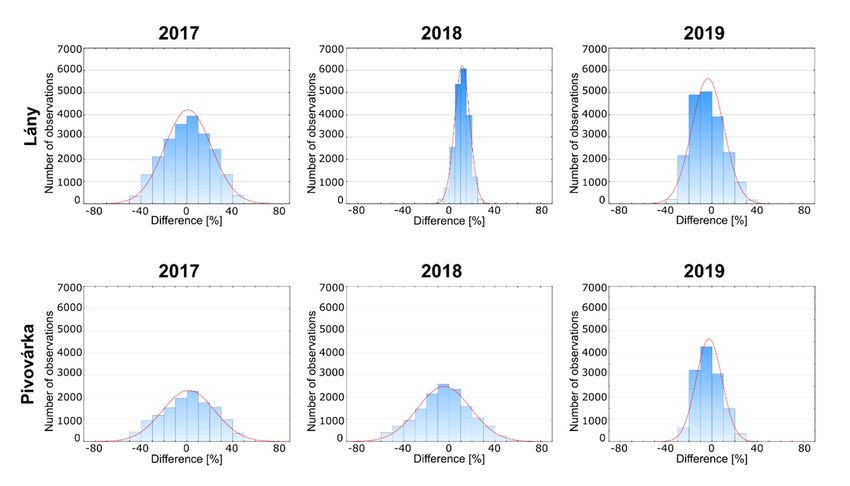
Remote Sens. 2020, 12, 1917                                                                                                 6 of 17

            Remote Sens. 2020, 12, x FOR PEER REVIEW                                                           6 of 19

                Figure 2. Schematic
      Figure 2. Schematic           workflow
                             workflow        of yield
                                        of yield      productivityzone
                                                  productivity     zone identification
                                                                        identification andand
                                                                                           computation in the form
                                                                                              computation      in the form of
                of a Unified Modeling Language (UML) activity diagram.
      a Unified Modeling Language (UML) activity diagram.
                 Yield productivity zones present values in percentages, identifying places with, for example,
     The abovementioned      indices
          60% or 140% of potential      need
                                    yield      to be computed
                                           in comparison           from value
                                                         to the average  the relevant    satellite
                                                                              for the given         data. Information
                                                                                              plot (Figure  3).
on farmer’s  parcels
          Farmers can (plots/LPIS    farmer’s
                       then adjust their         blocks)
                                          agronomical      is thebased
                                                       practices   second  input,
                                                                       on the spatialsince  it defines
                                                                                       variability        the
                                                                                                   of yield in geometry
of the plot boundary. Any deviation in the plot geometry and crop area (such as two crop species
within one plot boundary record) leads to an incorrect calculation of the plot variability type in one
vegetation season. If this were not the case, the production zones could not be computed for the whole
plot. The abovementioned indices are computed as variabilities within each plot. The potential yield
is then computed for each plot from the underlying EVI index (defined above) through Empirical
Bayesian Kriging (EBK)—a geospatial interpolation as defined in Pilz and Spöck [50] and Krivoruchko
and Gribov [51]—then smoothed to a spatial resolution of 5 m. The EBK enables values according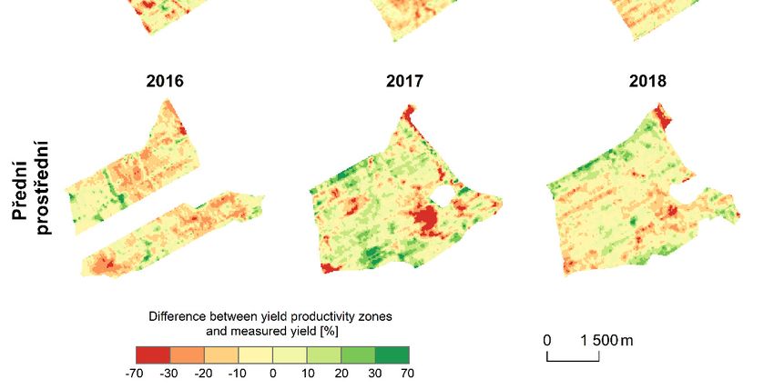
Remote Sens. 2020, 12, 1917 7 of 17
Kriging interpolation to be computed; however, the semivariograms differ from plot to plot thanks to
the Bayesian approach to semivariogram construction.
RemoteYield productivity
Sens. 2020, zones
12, x FOR PEER present values in percentages, identifying places with, for example,
REVIEW 60%
7 of 19
or 140% of potential yield in comparison to the average value for the given plot (Figure 3). Farmers can
general: prediction
then adjust and/or measurements.
their agronomical Note
practices based onthat
the farmers did not reach
spatial variability a consensus
of yield on prediction
in general: a strategy
for yield
and/or productivity Note
measurements. zones: “feed
that the did
farmers rich”
not(fertilizers primarily
reach a consensus oninto high productive
a strategy locations)
for yield productivity
versus
zones: “feed the rich” poor”(fertilizers
(fertilizersprimarily
primarilyinto
intohigh
lowproductive
productivelocations)
locations)versus
remain“feed
two the
opposite
poor”
approaches.
(fertilizers primarily into low productive locations) remain two opposite approaches.
Figure 3.
Figure Input data
3. Input data used
used for
for the
the analysis
analysis of
of yield
yield productivity
productivity zones: yield productivity
zones: yield productivity zone
zone
prediction derived from satellite images (left) and the map of yield measurements as computed
prediction derived from satellite images (left) and the map of yield measurements as computed by by aa
harvester (right).
harvester (right).
Yield productivity
Yield productivityzones
zonesareareanother
another form of data
form derived
of data fromfrom
derived periodic remote
periodic sensing.
remote The yield
sensing. The
(potential) is the integrator of landscape and climatic variability and, as such, provides
yield (potential) is the integrator of landscape and climatic variability and, as such, provides useful useful
information for
information for identifying
identifying management
management zones, zones, as
as defined
defined by
by Kleinjan
Kleinjan et
et al.
al. [52].
[52]. Yield
Yield productivity
productivity
zones represent the basic delineation of management zones for site-specific crop
zones represent the basic delineation of management zones for site-specific crop management, management, which
whichis
usually
is usuallybased
basedononyield
yieldmaps
mapsover
overthe thepast
pastseveral
severalyears.
years. As
As mentioned
mentioned before,
before, the
the presence of aa
presence of
complete series of yield maps for all plots is rare; thus, remotely sensed data are
complete series of yield maps for all plots is rare; thus, remotely sensed data are analyzed toanalyzed to determine
the plot variability
determine of crops through
the plot variability of crops vegetation indices. indices.
through vegetation
The proof-of-concept software solution
The proof-of-concept software solution for yield for yield productivity
productivity zone
zone identification
identification and
and computing
computing
was based on ArcGIS Desktop 10.3.1, developed by the ESRI (Environmental
was based on ArcGIS Desktop 10.3.1, developed by the ESRI (Environmental System Research System Research
Institute) corporation.
Institute) corporation.
2.3. Yield Productivity Zone Verification against Yield Measurements
2.3. Yield Productivity Zone Verification against Yield Measurements
Predictions in the form of yield productivity zones need to be confronted with the measured yield
Predictions in the form of yield productivity zones need to be confronted with the measured
data. The yield data are considered to be the most sensitive form of data at a farm [53]. Rostěnice Farm
yield data. The yield data are considered to be the most sensitive form of data at a farm [53]. Rostěnice
in the Czech Republic provided yield maps of cereals as the main crop for three plots between the
Farm in the Czech Republic provided yield maps of cereals as the main crop for three plots between
years 2016 and 2019, as depicted in Table 2. These yield maps were created by a CASE IH AXIAL
the years 2016 and 2019, as depicted in Table 2. These yield maps were created by a CASE IH AXIAL
FLOW 9120 harvester equipped with an AFS Pro 700 monitoring unit. The measurements are in
FLOW 9120 harvester equipped with an AFS Pro 700 monitoring unit. The measurements are in
GNSS-RTK quality (Global Navigation System of Systems—the Real Time Kinematics method provides
GNSS-RTK quality (Global Navigation System of Systems—the Real Time Kinematics method
a positional accuracy of better than 0.1 m; see [54]). The measurement frequency was set to one
provides a positional accuracy of better than 0.1 m; see [54]). The measurement frequency was set to
second (1 Hz). The harvesting width was equal to 9.15 m. The AFS Pro 700 monitoring unit was
one second (1 Hz). The harvesting width was equal to 9.15 m. The AFS Pro 700 monitoring unit was
calibrated at 15 randomly selected locations per field to produce yield maps that were as precise as
calibrated at 15 randomly selected locations per field to produce yield maps that were as precise as
possible. The monitoring of yield was conducted as on-the-go mapping by recording grain flow and
possible. The monitoring of yield was conducted as on-the-go mapping by recording grain flow and
moisture continuously over the whole plot area. The obtained data were later filtered to detect and
moisture continuously over the whole plot area. The obtained data were later filtered to detect and
remove erroneous values, outliers, spatial deviations, etc.; the data were also subsequently interpolated,
remove erroneous values, outliers, spatial deviations, etc.; the data were also subsequently
following the approach described in our previous papers [55,56]).
interpolated, following the approach described in our previous papers [55,56]).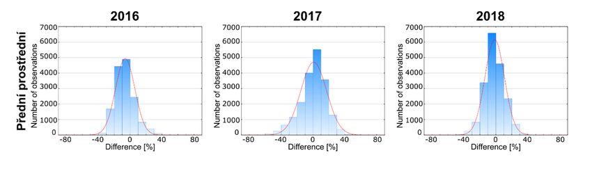
Remote Sens. 2020, 12, 1917                                                                                     8 of 17

      Table 2. Harvesting details for each campaign: identification of a plot, date of harvest, cultivated crop,
      cultivated acreage, number, and average density of measurements from the field harvester.

                                                                  Acreage        Number of         Measurements
        Plot            Date of Harvest           Crop
                                                                   (Ha)         Measurements        per Hectare
                              14 July 2017   wheat winter           70.4            37,115              527.2
 “Lány” plot (ID
                              3 July 2018     oilseed rape          70.4            43,141              612.8
    2401/20)
                              21 July 2019   wheat winter           70.4            23,851              338.8
                              14 July 2017    barley spring         44.5            23,552              454.7
  “Pivovárka”
                       19 September 2018          corn              44.5            44,433              998.5
 plot (ID 2401/9)
                              18 July 2019    barley spring         44.5            16,038              360.4
      “Přední           24 October 2016     wheat winter           61.2            16,587              271.0
     prostřední”
                              14 July 2017    barley spring         61.2            25,580              418.0
      plot (ID
      2401/12)           11 October 2018     barley Spring          61.2            19,381              316.7

     A geospatial correlation between the predicted yield productivity zones on the one hand and the
yield measurement data on the other hand was performed using the following geospatial procedures:

1.     Both the yield productivity zones (predictions) and the yield measurements (reference data)
       were transformed into relative values by means of a linear function. This approach enables the
       comparability of predictions with reference data.
2.     To visualize and describe the spatial patterns of the differences between the yield productivity
       zones and yield measurements, map algebra was used, especially the geospatial subtraction. Map
       algebra provides insights on variances between the values in raster data that are overlapping [57].
       The geospatial subtraction was used as defined in Equation (2).
3.     The following steps were applied prior to correlation. The data were transformed from raster
       to discrete reference points. Reference points were created as centroids of yield measurement
       pixels (values were stored as attributes), and the values of predicted yield were extracted to
       another attribute. These reference points on the one hand and the concave hull of the filtered
       field harvester data on the other hand were intersected [55]. Concave hulls were created by the
       Aggregate Points function [58], with an aggregation distance of 60 m (based on the analyzed data
       and field geometry characteristics) and minor shape modifications due to aggregations outside of
       the area of the plot (northwest of the Lány plot).

                                                   dy = yz − ym,                                                   (2)

where:
   dy: difference in the predicted and measured yields,
   yz: yield productivity zones (predictions),
   ym: yield measurements (reference data).

4.     Intersection between the reference points and concave hull of the filtered field harvester data was
       performed because of the following reasons:

       a.      The raster applied in this study did not have equal coverage, and therefore “null” values
               occurred in attributes.
       b.      The extrapolated values of yield measurements occur at the edges of a plot, as they are:

               i.       artificially calculated, based more on (settings of) software algorithms than actual
                        data measurements;
               ii.      influenced by the harvesting strategy (for more information, see [55]).
Remote Sens. 2020, 12, 1917 9 of 17
Remote Sens. 2020, 12, x FOR PEER REVIEW 9 of 19
c. Non-credible values of the yield potential (e.g., the “Pivovárka” plot in 2018) rationale
remainsi. an open question—a working theory counts the surrounding vegetation
artificially calculated, based more on (settings of) software algorithms than actual that
influences thedata
evapotranspiration
measurements; conditions. This working theory will be pursued further
ii.
as a subject influenced
for ongoing by the harvesting strategy (for more information, see [55]).
research.
c. Non-credible values of the yield potential (e.g., the “Pivovárka” plot in 2018) rationale
5. Finally, geospatial data—in other words, reference points with yield values as attributes—were
remains an open question—a working theory counts the surrounding vegetation that
transformed influences
into tables, and the Pearson
the evapotranspiration correlation
conditions. coefficient
This working (Pearson’s
theory will be r) [59] was
pursued further
used for calculating the
as a subject for correlation between the predicted yield productivity and the yield
ongoing research.
5. Finally,
measurement geospatial data—in other words, reference points with yield values as attributes—were
data.
transformed into tables, and the Pearson correlation coefficient (Pearson’s r) [59] was used for
calculating the
For the verification, thecorrelation
following between the predicted
software yieldused:
tools were productivity
ArcGIS and the yield 10.3.1
Desktop measurement
(for geospatial
data.
subtraction, to create concave hulls and maps) and Statistica (to calculate the correlation coefficients
For the verification, the following software tools were used: ArcGIS Desktop 10.3.1 (for
and to create graphs).
geospatial subtraction, to create concave hulls and maps) and Statistica (to calculate the correlation
coefficients and to create graphs).
3. Results
3. Results
Yield productivity zones may be understood as a prediction, while yield measurements are used
as the referenceYield
dataproductivity zones may
for validation. be understood
The geospatial as distribution
a prediction, while yield measurements
of measured are used between
yield values
as the reference data for validation. The geospatial distribution of measured yield values between
plots at Rostěnice Farm is depicted in Table 2.
plots at Rostěnice Farm is depicted in Table 2.
The results Theofresults
the geospatial subtraction
of the geospatial subtractionofofyield productivity
yield productivity zones
zones (prediction)
(prediction) from yield
from yield
measurements (reference
measurements data) are
(reference data)depicted in in
are depicted Figure
Figure4.4.
Figure 4. Differences between the yield productivity zone values and yield measurements: subtraction
of the yield productivity zones (prediction) from yield measurements (reference data).
Results depicted in Table 3 and Figure 5 demonstrate variabilities (mean, minimum and maximum
values, standard deviation) in yield productivity zones on the one hand and variabilities in the
measured yield on the other hand. Differences between the values on yield productivity zones and
measured yield are provided with equal statistical characteristics. All the information illustrates the
variabilities of three plots for three years.and measured yield are provided with equal statistical characteristics. All the information illustrates
the variabilities of three plots for three years.
The differences between the yield productivity zones and the measured yield confirm that the
prediction provided by the yield productivity zones led to an overestimation in five cases out of nine
and an
Remote underestimation
Sens. 2020, 12, 1917 in four cases out of nine. The differences in the yield prediction compared to
10 of 17
the measured values were up to 5% in seven cases. The only two differences in the predicted and
measured yield were as follows: (1) the Přední Prostřední plot resulted in a 6.66% overestimation in
2016,Tablewhile Statistical
3. (2) the Lány characteristics
plot resulted forinthe reference
a 10.83% points used for in
underestimation the2018.
comparison of differences
between the yield productivity zones and the measured
Standard deviations on the one hand as well as the extent of (minimumyield. Note that the “N” column depicts thevalues
and maximum)
number of reference points that were used for interpolation and intersected by the concave hulls; this
on the other hand were, in all cases, higher than the yield values measured by a field harvester. In
means the number of reference points in Table 3 differs from the number of measured points in Table 2.
other words, in all cases the data measured under real conditions showed a higher variation, meaning
greater Plot
local differences,
Year N
than Yield
the (model of)[%]
Productivity predictions.Measured
FigureYield
3 shows
[%] that phenomena
Differencesuch
[%] as the
intervals used in the legendMean Min. Max.
are equal for bothStdv Mean Min. Max.
prediction using the yield Stdv Mean Min.
productivity Max. Stdv
zones and the
2017 21,561 100.79 83.00 116.00 4.43 100.08 44.88 155.23 21.49 0.71 −53.30 53.29 20.33
measured
“Lány” plotyield (in Figure 3 for the Pivovárka plot in 2018). The Pivovárka plot in 2018, the Pivovárka
2018 20,463 100.40 85.00 113.00 4.47 89.57 73.66 119.17 6.53 10.83 −20.17 36.16 6.56
(ID 2401/20)
plot in 2017, and the Lány
2019 19,731 plot in 2017
99.72 82.00 resulted also in
114.00 5.26 the largest
103.57 standard
64.20 135.22 13.73deviations: 23.13%,
−3.85 −38.18 39.8022.71%,
13.97
and 20.33%,
“Pivovárka” plot respectively. All three plots were also characterized by a clear spatial pattern. The
2017 13,141 97.87 83.00 121.00 5.16 96.83 50.13 148.88 22.57 1.04 −58.93 56.87 22.71
2018 14,420 98.61 83.00 114.00 5.13 103.46 34.14 166.76 25.20 −4.85 −68.96 62.67 23.13
agronomical season
(ID 2401/9)
2019 of 2017100.03
13,078 was marked by high
84.00 114.00 4.37local differences
102.98 for all11.41
69.29 130.47 three−2.94
plots −32.55
within 35.71
this study.
11.27
Figure
“Přední 5 presents
2016 14,912histograms
97.99 of the differences between
77.00 122.00 8.56 104.65 55.60 122.77 the yield productivity
10.50 −6.66 −39.63 47.01and
zones the
12.05
prostřední” plot 2017 19,071 98.17 80.00 126.00 6.29 97.71
measured yield for all three plots and three years portrayed in Figure 4. 53.38 147.95 16.45 0.46 −57.44 52.23 16.19
(ID 2401/12) 2018 18,856 97.80 77.00 116.00 6.03 99.71 53.38 146.87 13.23 −1.91 −51.88 41.00 12.21
Figure 5. Histograms of differences between the yield productivity zones and the measured yield. Note:
the histogram for the Lány field in 2018 was modified to increase readability, meaning the intervals of
the differences are equal to 5% instead of 10% as in the other histograms.
The differences between the yield productivity zones and the measured yield confirm that the
prediction provided by the yield productivity zones led to an overestimation in five cases out of nine
and an underestimation in four cases out of nine. The differences in the yield prediction compared
to the measured values were up to 5% in seven cases. The only two differences in the predicted and
measured yield were as follows: (1) the Přední Prostřední plot resulted in a 6.66% overestimation in
2016, while (2) the Lány plot resulted in a 10.83% underestimation in 2018.
Standard deviations on the one hand as well as the extent of (minimum and maximum) values on
the other hand were, in all cases, higher than the yield values measured by a field harvester. In otherRemote Sens. 2020, 12, 1917 11 of 17
words, in all cases the data measured under real conditions showed a higher variation, meaning greater
local differences, than the (model of) predictions. Figure 3 shows that phenomena such as the intervals
used in the legend are equal for both prediction using the yield productivity zones and the measured
yield (in Figure 3 for the Pivovárka plot in 2018). The Pivovárka plot in 2018, the Pivovárka plot in 2017,
and the Lány plot in 2017 resulted also in the largest standard deviations: 23.13%, 22.71%, and 20.33%,
respectively. All three plots were also characterized by a clear spatial pattern. The agronomical season
of 2017 was marked by high local differences for all three plots within this study.
Remote Sens. 2020, 12, x FOR PEER REVIEW 13 of 19
Figure 5 presents histograms of the differences between the yield productivity zones and the
measured yield for all three plots and three years portrayed in Figure 4.
Figure 6 depicts scatter plots in order to demonstrate the extents of all the differences between the
Figure 6 depicts scatter plots in order to demonstrate the extents of all the differences between the
predicted yield productivity zones and the measured yield. The purpose of Figure 6 is to bring a more
predicted yieldof
complex point productivity zones and
view in comparison tothe measured
Table yield. 5,
3 and Figures The purpose
which of Figure
operate “only”6with
is tomean
bringvalues.
a more
complex point of view in comparison to Table 3 and Figure 5, which operate “only” with mean values.
Figure 6. Scatter plots showing the relationships between the yield productivity zones and the
Figure 6. Scatter
measured yield. plots showing the relationships between the yield productivity zones and the measured
yield.
Table 4 depicts the Pearson correlation coefficient (Pearson’s r) and probability values (p) between
Table 4 yield
the predicted depicts the Pearson
productivity correlation
zones and the coefficient (Pearson’s
measured yield for all r)
theand probability
reference pointsvalues (p)
in all the
between the
measured predicted
years. yield productivity
The correlation zones andasthe
has been identified measuredsignificant
statistically yield for all
forthe
all reference points
the plots in in
all the
all theatmeasured
years years. Thelevel.
a 95% significance correlation has been identified as statistically significant for all the plots
in all the years at a 95% significance level.
Table 4. Pearson correlation coefficient (Pearson’s r) at a 95% significance level. Note that “N/A” means
“not applicable”, as field machinery measurements were not available for such a combination of a plot and
year.
“Lány” Plot (ID 2401/20) “Pivovárka” Plot (ID 2401/9) “Přední prostřední” Plot (ID 2401/12)
Year
r r r
2016 N/A N/A 0.214
2017 0.365 0.086 0.124
2018 0.347 0.470 0.362Remote Sens. 2020, 12, 1917 12 of 17
Table 4. Pearson correlation coefficient (Pearson’s r) at a 95% significance level. Note that “N/A” means
“not applicable”, as field machinery measurements were not available for such a combination of a plot
and year.
“Pivovárka” Plot “Přední prostřední”
“Lány” Plot (ID 2401/20)
Year (ID 2401/9) Plot (ID 2401/12)
r r r
2016 N/A N/A 0.214
2017 0.365 0.086 0.124
2018 0.347 0.470 0.362
2019 0.146 0.222 N/A
4. Discussion
Yield productivity zones were evaluated as a feasible way of discovering the areas within a plot
with higher-than-average and lower-than-average yields. The identification and computation of yield
productivity zones is crucial for increasing the yield while minimizing the environmental pollution
from agricultural activities by reducing the amount of fertilizer(s) added to the soil [60,61]. The authors
would also like to emphasize that yield productivity zones are not a comprehensive solution but an
additional input for further modelling, processes and decision-making.
A qualitative evaluation of the yield productivity zone concept was also conducted, in addition to
the geospatial and statistical evaluation described in the results section. The qualitative evaluation
was in the form of discussions with farmers, agronomists, and agro-scientists at a dozen farms in
Europe (Austria, the Czech Republic, Germany, Latvia, and Spain). The qualitative verification was
performed for farms without detailed yield measurements in the form of maps. However, the surveyed
farmers, agronomists, and agro-scientists were employees who had worked on the evaluated plots
for a considerable amount of time—in many cases for decades—and were therefore well-acquainted
with the geospatial variations within, as well as between, the plots. It was concluded that the yield
productivity zones correctly identify spatial patterns—in other words, zones with higher-than-average
and lower-than-average yields within a plot. At the same time, the yield productivity zones were
understood by the surveyed farmers, agronomists, and agro-scientists as one of the inputs for planning
operations; other kinds of input varying in importance year to year included the weather, weeds,
and pests. In general, the yield productivity zones are recognized as a valuable source of information;
however, this information needs to be coordinated with the particularities of the agronomical season,
including the kind of crop cultivated.
Yield productivity zones have been computed in the way described in this paper for the last four
years (2016–2019). Unfortunately, yield measurements were not available for the same time period.
Only partial information is therefore available on the geospatial distribution of yield measurements
during various years. We came to the following conclusions when comparing the sums of the actual
yields on the one hand and yield productivity zones (predictions) on the other hand for each plot at a
dozen monitored farms in Europe from 2014. In terms of yield, the geospatial variations within the
plots were minimal during rich years. It was argued by farmers/agronomists/agro-scientists that the
monitored cereals would have grown anyway during such rich years (with optimal temperatures,
rainfall, etc.). On the contrary, the pattern as depicted by yield productivity zones (prediction) became
more clear in terms of yield during the poor years.
Uncertainties lie in areas of spatial and temporal resolutions:
• The spatial resolution of satellite data caused data inconsistencies between the Sentinel and
Landsat missions. The yield productivity zones were calculated at the spatial resolution of 5 m,
which meant a smoothening from the original spatial resolution of 30 m in the case of the Landsat
data and from 20 m in the case of the Sentinel data.Remote Sens. 2020, 12, 1917 13 of 17
• The spectral resolution of Sentinel-2A, Sentinel-2B, and Landsat 8 varies as these sensors differ in
the ranges of recorded radiation. The presented paper deals with eight years’ series, comprising
combinations of all three sensors. A more detailed analysis is beyond the scope of this paper.
• The temporal resolution for satellite data causes inconsistencies between the Sentinel-2A/B (5 days)
and Landsat-8 (16 days) missions. Between 2016 and 2019, data from both the satellite missions
were available; the Landsat mission satellite data are the only sufficient and freely available data
older than 6 May 2016 for the study area.
• The spatial resolution for yield measurements: the positional error was influenced by two
factors—the speed of the harvester and the delay between the collection of grain and the
computation of the respective yield [55]. Theoretically, the maximum positional error for the
yield measurements could be up to 18.6 m, although such a high value would be improbable in
practice. The yield measurements from harvesters in our study reached a spatial resolution of up
to 9.15 m (operational harvesting width) to 3.1 m (measurements each two seconds for average
speed 1.55 m·s−1 ).
• The temporal resolution for the yield measurements: the time period for the monitoring of farm
machinery telemetry should be the same as that for yield productivity zones—i.e., the last 8 years.
Such a requirement could not be met for the experiments conducted. Only three consecutive years
measurements for three plots were available at Rostěnice Farm.
Computing and expressions including the visualizations of uncertainties remain an open issue.
Another subject of debate is the processing of data from headland areas occurring mainly at the
edges of the plots. The concave hulls approach used for yield measurements implies less headland
areas and less filtering. It is therefore assumed that the results, too, are generally more accurate.
However, this conclusion is closely related to the harvesting strategy [55].
The use of the real-time tracking of farm machinery was mentioned in the introduction is one of
the prerequisites for any kind of precision farming application. In the scope of the sensor observation
domain, a piece of machinery is equivalent to a set of sensors deployed on a mobile carrier. On the
one hand, machinery can be monitored passively in order to collect data about the machinery itself
and about the processed plot; on the other hand, machinery can be monitored actively in order to
navigate the machinery and to control the batching of fertilizer, pesticides, or other substances at
desired locations. Data derived from machinery tracking can supplement the source dataset for yield
productivity zone calculations due to the more frequent use of machinery on the same plot.
5. Conclusions
Studies on yield predictions are becoming increasingly common. In contrast, studies comparing
predictions computed from satellite images with yield measurements at fully operational farms are
rare since (detailed) yield data are the most sensitive kind of farm data. The non-openness of yield
data is even worse with respect to accessing yield maps that depict the geospatial variations in yield
within a plot—that is to say, maps with yield measurements from harvesters in our study reaching
up to a spatial resolution of 9.15 m (operational harvesting width) to 3.1 m (measurements each two
seconds for average speed 1.55 m·s−1 ).
The conducted study proved correlations between the predicted yield productivity zones and the
measured yield for all three plots in all three years at a 95% significance level. Standard deviations as
well as the extent of (minimum and maximum) values are in all cases higher than the yield values
measured by a field harvester. The following statements are valid for the conducted study when
taking into account the resulting mean values. In seven cases, the differences in yield predictions
compared to the measured values were up to 5%. The prediction overestimated the yield by 6.66%
in one case and underestimated it by 10.83% in another case. Moreover, a qualitative evaluation by
farmers/agronomists/agro-scientists has also demonstrated the credibility of yield productivity zone
identification as well as its geospatial distribution across six years (from 2014 to 2019) at a dozen farms
in seven countries (Austria, the Czech Republic, Latvia, Germany, Poland, Spain and Turkey).Remote Sens. 2020, 12, 1917 14 of 17
As the research conducted in the FOODIE and SIEUSOIL projects has confirmed, farmers are
willing to use predictions in the form of yield productivity zones as an input for their decision-making.
Geospatial and statistical evaluations demonstrated the validity of yield productivity zones as an
instrument for predicting long-term areas of high and low yield, meaning areas where crop yield has
for several years been significantly above/below the yield average for the whole plot.
Yield productivity zones are used throughout the whole vegetation season primarily because
of fertilizer application planning. Moreover, the presented yield productivity zones concept has
already been successfully registered under Phase 8 of the Global Earth Observation System of Systems
(GEOSS) Architecture Implementation Pilot in order to support the wide variety of requirements that are
primarily aimed at agricultural pollution monitoring, typically pollution by fertilizer/pesticide residues.
Supplementary Materials: The following are available online at http://www.mdpi.com/2072-4292/12/12/1917/s1,
Table S1: Overview of satellite imagery from Landsat mission used for the calculation of yield zones; Table S2:
Overview of satellite imagery from Sentinel-2 mission used for the calculation of yield zones.
Author Contributions: T.Ř. together with V.L. and P.Š. outlined the state of the art and designed the methods;
the description of results and statistical evaluation were undertaken by T.Ř., T.P., L.H., V.L., and F.L.; Š.L. created
the UML workflow; T.Ř. and L.H. contributed to the discussion section; T.Ř. wrote the conclusions section and
abstract. All authors have read and agreed to the published version of the manuscript.
Funding: This paper is part of a project that has received funding from the European Union’s Horizon 2020
research and innovation program under grant agreement No. 818346, called “Sino-EU Soil Observatory for
intelligent Land Use Management” (SIEUSOIL).
Acknowledgments: The authors would like to thank all persons from the Rostěnice Farm who participated in the
study, from the drivers of farm machinery to the farm’s agronomists and management.
Conflicts of Interest: The authors declare no conflict of interest.
References
1. Auernhammer, H. Precision farming—The environmental challenge. Comput. Electron. Agric. 2001, 30, 31–43.
[CrossRef]
2. D5.1.2: Pilots Description and Requirements Elicitation Report, FOODIE Project Consortium. Internal Project
Document. 2015; p. 59. Available online: http://www.foodie-project.eu/public/20150619173124.pdf (accessed
on 23 April 2020).
3. D1.1: Agricultural Pilot Definition, DataBio Project Consortium. Internal Project Document. 2017; p. 155.
Available online: https://www.databio.eu/wp-content/uploads/2017/05/DataBio_D1.1-Agriculture-Pilot-
Definition_v1.1_2018-04-26_LESPRO.pdf (accessed on 23 April 2020).
4. Palma, R.; Reznik, T.; Esbri, M.; Charvat, K.; Mazurek, C. An INSPIRE-Based Vocabulary for the Publication
of Agricultural Linked Data. In Ontology Engineering—Lecture Notes in Computer Science, Proceedings of the
International Experiences and Directions Workshop on OWL 2016, Bologna, Italy, 20 November 2016; Tamma, V.,
Dragoni, M., Gonçalves, R., Ławrynowicz, A., Eds.; Springer: Cham, Germany, 2016; pp. 124–133. [CrossRef]
5. Feiden, K.; Kruse, F.; Reznik, T.; Kubicek, P.; Schentz, H.; Eberhardt, E.; Baritz, R. Best Practice
Network GS SOIL Promoting Access to European, Interoperable and INSPIRE Compliant Soil Information.
In Environmental Software Systems, Proceedings of the Frameworks of eEnvironment, IFIP Advances in Information
and Communication Technology, Vol. 359, ISESS 2011, Brno, Czech Republic, 27–29 June 2011; Hrebicek, J.,
Schimak, G., Denzer, R., Eds.; Springer: Heidelberg, Germany, 2011; pp. 226–234. [CrossRef]
6. Stampach, R.; Kubicek, P.; Herman, L. Dynamic visualization of sensor measurements: Context based
approach. Quaest. Geogr. 2015, 34, 117–128. [CrossRef]
7. Reznik, T.; Lukas, V.; Charvat, K.; Charvat, K., Jr.; Horakova, S.; Krivanek, Z.; Herman, L. Monitoring of
In-Field Variability for Site Specific Crop Management through Open Geospatial Information. In ISPRS
Archives of the Photogrammetry, Remote Sensing and Spatial Information Sciences; Halounová, L., Ed.; Copernicus
GmbH: Gottingen, Germany, 2016; Volume XLI-B8, pp. 1023–1028. [CrossRef]
8. Evans, L.T.; Fischer, R.A. Yield productivity zones: Its definition, measurement, and significance. Crop Sci.
1999, 39, 1544–1551. [CrossRef]Remote Sens. 2020, 12, 1917 15 of 17
9. Nemenyi, M.; Mesterhazi, P.A.; Pecze, Z.; Stepan, Z. The role of GIS and GPS in precision farming.
Comput. Electron. Agric. 2003, 40, 45–55. [CrossRef]
10. Lobell, D.B.; Cassman, K.G.; Field, C.B. Crop yield gaps: Their importance, magnitudes, and causes.
Annu. Rev. Environ. Resour. 2009, 34, 179–204. [CrossRef]
11. Van Wart, J.; Kersebaum, K.C.; Peng, S.; Milner, M.; Cassman, K.G. Estimating crop yield productivity zones
at regional to national scales. Field Crop. Res. 2013, 143, 34–43. [CrossRef]
12. Van Ittersum, M.K.; Cassman, K.G.; Grassini, P.; Wolf, J.; Tittonell, P.; Hochman, Z. Yield gap analysis with
local to global relevance—A review. Field Crop. Res. 2013, 143, 4–17. [CrossRef]
13. Chen, Y.; Zhang, Z.; Tao, F.; Wang, P.; Wei, X. Spatio-temporal patterns of winter wheat yield productivity
zones and yield gap during the past three decades in north China. Field Crop. Res. 2017, 206, 11–20. [CrossRef]
14. Bauer, M.E. The role of remote sensing in determining the distribution and yield of crops. In Advances in
Agronomy; Brady, N.C., Ed.; Academic Press: New York, NY, USA, 1975; Volume 27, pp. 271–304. [CrossRef]
15. Doraiswamy, P.C.; Hatfield, J.L.; Jackson, T.J.; Akhmedov, B.; Prueger, J.; Stern, A. Crop condition and yield
simulations using Landsat and MODIS. Remote Sens. Environ. 2004, 92, 548–559. [CrossRef]
16. Lobell, D.B. The use of satellite data for crop yield gap analysis. Field Crop. Res. 2013, 143, 56–64. [CrossRef]
17. Quarmby, N.A.; Milnes, M.; Hindle, T.L.; Silleos, N. Use of multi-temporal NDVI measurements from
AVHRR data for crop yield estimation and prediction. Int. J. Remote Sens. 1993, 14, 199–210. [CrossRef]
18. Bolton, D.K.; Friedl, M.A. Forecasting crop yield using remotely sensed vegetation indices and crop phenology
metrics. Agric. For. Meteorol. 2013, 173, 74–84. [CrossRef]
19. Sakamoto, T.; Gitelson, A.A.; Arkebauer, T.J. Near real-time prediction of U.S. Corn yields based on time-series
MODIS data. Remote Sens. Environ. 2014, 147, 219–231. [CrossRef]
20. Johnson, D.M. An assessment of pre- and within-season remotely sensed variables for forecasting corn and
soybean yields in the United States. Remote Sens. Environ. 2014, 141, 116–128. [CrossRef]
21. Zhao, Y.; Potgieter, A.B.; Zhang, M.; Wu, B.; Hammer, G.L. Predicting Wheat Yield at the Field Scale by
Combining High-Resolution Sentinel-2 Satellite Imagery and Crop Modelling. Remote Sens. 2020, 12, 1024.
[CrossRef]
22. Thenkabail, P.S. Biophysical and yield information for precision farming from near-real-time and historical
Landsat TM images. Int. J. Remote Sens. 2003, 24, 2879–2904. [CrossRef]
23. Gu, Y.; Wylie, B.K. Developing a 30-m grassland productivity estimation map for central Nebraska using
250-m MODIS and 30-m Landsat-8 observations. Remote Sens. Environ. 2015, 171, 291–298. [CrossRef]
24. Reznik, T.; Charvat, K., Jr.; Charvat, K.; Horakova, S.; Lukas, V.; Kepka, M. Open Data Model for (Precision)
Agriculture Applications and Agricultural Pollution Monitoring. In Proceedings of the Enviroinfo and ICT
for Sustainability, Copenhagen, Denmark, 7–9 September 2015; Johannsen, V.K., Jensen, S., Wohlgemuth, V.,
Preist, C., Eriksson, E., Eds.; Atlantis Press: Paris, France, 2015; Volume 22, pp. 97–107. [CrossRef]
25. Pierce, F.J.; Nowak, P. Aspects of precision agriculture. In Advances in Agronomy; Sparks, D.L., Ed.; Academic
Press: New York, NY, USA, 1999; Volume 67, pp. 1–85. [CrossRef]
26. Sun, W.; Whelan, B.; McBratney, A.B.; Minasny, B. An integrated framework for software to provide yield
data cleaning and estimation of an opportunity index for site-specific crop management. Precis. Agric. 2013,
14, 376–391. [CrossRef]
27. Bongiovanni, R.; Lowenberg-Deboer, J. Precision agriculture and sustainability. Precis. Agric. 2004, 5, 359–387.
[CrossRef]
28. Gebbers, R.; Adamchuk, V.I. Precision agriculture and food security. Science 2010, 327, 828–831. [CrossRef]
29. Zhang, N.; Wang, M.; Wang, N. Precision agriculture—A worldwide overview. Comput. Electron. Agric. 2002,
36, 113–132. [CrossRef]
30. Reznik, T.; Lukas, V.; Charvat, K.; Charvat, K.jr.; Krivanek, Z.; Kepka, M.; Herman, L.; Reznikova, H. Disaster
Risk Reduction in Agriculture through Geospatial (Big) Data Processing. ISPRS Int. J. Geo-Inf. 2017, 6, 238.
[CrossRef]
31. Call for Participation in GEOSS Architecture Implementation Pilot (AIP-8). 2015. Available online:
https://www.earthobservations.org/documents/cfp/201501_geoss_cfp_aip8.pdf (accessed on 17 April 2020).
32. United States Environmental Protection Agency 2015 Summary of the Clean Water Act 33 U.S.C. §1251 et
seq. 1972. Available online: http://www2.epa.gov/laws-regulations/summary-clean-water-act (accessed on
23 April 2020).You can also read