Optimization Model of Taxi Fleet Size Based on GPS Tracking Data - MDPI
←
→
Page content transcription
If your browser does not render page correctly, please read the page content below
sustainability

Article
Optimization Model of Taxi Fleet Size Based on GPS
Tracking Data
Yang Yang 1,2,3, * , Zhenzhou Yuan 1,3 , Xin Fu 4, *, Yinhai Wang 2 and Dongye Sun 3
 1   MOE Key Laboratory for Urban Transportation Complex Systems Theory and Technology, Beijing Jiaotong
     University, Beijing 100044, China; zzyuan@bjtu.edu.cn
 2   Department of Civil and Environmental Engineering, University of Washington, More Hall, University of
     Washington, Seattle, WA 98195, USA; yinhai@uw.edu
 3   School of Traffic and Transportation, Beijing Jiaotong University, Beijing 100044, China;
     14114218@bjtu.edu.cn
 4   School of Economics and Management, Chang’an University, Middle section of South Second Ring Road,
     Xi’an 710064, China
 *   Correspondence: 14114222@bjtu.edu.cn (Y.Y.); fuxin@chd.edu.cn (X.F.)

 Received: 11 December 2018; Accepted: 28 January 2019; Published: 30 January 2019

 Abstract: A reasonable taxi fleet size has a significant impact on the satisfaction of urban traffic
 demand, the alleviation of urban traffic congestion, and the stability of taxi business groups.
 Most existing studies measure the overall scale by using macro indices, and few studies are from
 the micro level. To meet the transportation demand for taxis, mitigating the mismatch between
 taxi supply and demand, this research proposes an urban taxi fleet size calculating model based on
 GPS tracking data. Firstly, on the basis of road network segmentation, the probability model of a
 passenger taxi-taking a road section as a unit is built to evaluate the difficulty of taxi-taking on a road
 section. Furthermore, a user queuing model is built for the “difficult to take a taxi” road section in
 the peak period, and the service mileage required by potential taxi users is calculated. After that,
 a transportation capacity measurement model is built to estimate the number of taxis required in
 different time periods, Finally, the income constraint model is used to explain the impact of different
 vehicle fleet sizes on the income of taxi groups, so as to provide a reference for the determination of
 the final fleet size. The model is applied to data from Xi’an. The calculation results are based on data
 from May 2014, and show that the scale of taxi demand is about 654–2237, and after considering the
 impact of different fleet size increases on income, when the income variation index is limited to 0.10,
 i.e., the decrease of drivers’ income will not exceed 10%, an increase of 1286 taxis will be able to meet
 66% of the unmet demand in the peak period. The conclusion indicates that the model can effectively
 calculate the required fleet size and formulate the constraint solutions. This method provided can be
 considered as a support for formulating the regulation strategy of an urban taxi fleet size.

 Keywords: taxi; GPS tracking data; optimization fleet size model

1. Introduction
      Taxis are one of the main modes of travel in cities. Although there are great differences between
taxis and public transportation in terms of transport capacity, its flexibility and personalized service are
important characteristics to meet the needs of urban transportation [1]. In the process of taxi operation,
how to regulate the reasonable fleet size of taxis to meet residents’ travel needs without causing too
much traffic congestion and affecting the operating income of traditional taxi operators is an important
premise for strategy formulation. On the one hand, if the amount of fleet investment is too small, where
supply is less than demand, it will inevitably cause travel inconvenience and difficulties in taking a taxi.

Sustainability 2019, 11, 731; doi:10.3390/su11030731                     www.mdpi.com/journal/sustainability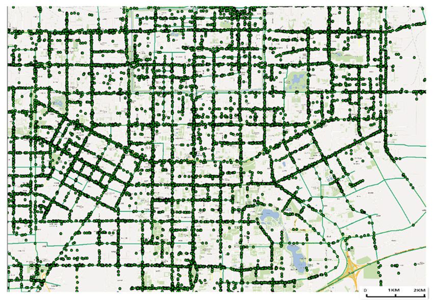
Sustainability 2019, 11, 731                                                                       2 of 19

When the amount of fleet investment is too much, the income of existing groups will decline, and lead
to the aggravation of urban traffic congestion, the increase of citizens’ travel costs, and even negative
social impact [2]. Therefore, a proper taxi fleet size management strategy that balances passengers’
benefits (measured by taxi fare and average waiting time) and operation efficiency (measured by taxi
operation cost and drivers’ income) is essential to mitigate the supply-demand mismatch, improve the
transportation environment, and increase the transportation satisfaction of residents.
      Many studies have focused on the relationship between the reasonable operation fleet scale of
the taxi and its travel rules: Douglass C. North [3] introduced an aggregation model that treated unit
time taxi operation cost as a constant. The model revealed that the passengers’ demand for a taxi
is a decreasing function of average taxi fare and expected wait time, which is in reverse correlation
to the deadhead time. Although this model did not take the spatial structure of a taxi market into
account, it was adopted by several economists since it succinctly summarized the characteristics of
this market, leading to continuous improvement of research in this field. The research on taxi fleet
size allocation and demand forecasting has been a hot spot in this field: Khaled Abbas, based on
summarizing the existing studies on taxi fleet size allocation, takes a hypothetical city as an example.
Three models, “future taxi fleet size based on taxi availability index”, “taxi fleet requirements based
on hara taxi demand model”, and “generic algorithm for estimation of taxi fleet size”, are applied
to calculate the fleet size of future taxi allocation and demand prediction [4]. Specifically, for the
optimization of the relationship between taxi fleet size and revenue, Baozhen Yao et al. [5] established
a bilevel programming model to solve this problem. The lower model is the demand function model,
which calculates the fleet size demand according to the given capacity configuration and ticket price.
The results show that the increase of vehicle configuration size can attract potential demand, but the
size of attraction mainly depends on the waiting time of passengers and taxi fares, indicating that the
three are interrelated and have an impact, which should be taken into account in the study. While
traditional taxis are impacted by emerging rental services like Uber and Lyft, Satish v. Ukkusuri and
Zhang [6] developed a model framework to study market research based on decentralized equilibrium
in order to obtain an optimal pricing and scale of taxi allocation in a given urban area. Its case study,
based on data from New York City, shows that the taxi market at the time may have been oversupplied
and underpriced, echoing other match research and the fact that New York taxi prices rose in 2012.
Based on two Stackelberg games, two different development strategies are proposed to cope with
the anticipated changes in a taxi system, such as the price and quantity elasticity of taxi demand,
demand difference level, average taxi speed, passenger waiting time value and taxi service coverage.
When the problem focuses on solving urban congestion, complying with the policy of energy saving
and emission reduction, and considering the taxi pooling efficiency of passengers and taxi driver
income, taxi pooling, and ride share are important measures to solve the problem. Some scholars
have also conducted in-depth studies on taxi pooling and ride share: Wang, etc. [7] built an analytical
model for taxi volume quantification based on urban taxi demand-supply balance theory and utility
theory. All parameters, such as taxi effective mileage, deadhead rate, average daily operation time and
average operation speed, was weighted in calculation and modeling. Yang and Sun [8,9] used entropy
weight and the weight optimization method in their traffic transportation models respectively.
      These studies rely on the statistics of distance and time gathered from residents’ travel surveys,
which oftentimes provides data that is less accurate and results in a model that is inapplicable in
practical applications in large cities. In addition, there is no complete travel data for small and
medium-sized cities to calculate the total scale of travel. When calculating the total demand of taxi
in the research method, the geographic information attributes of taxi operation trajectory and urban
residents’ travel demand are not considered. As for the use of theories and methods, as well as
the processing and mastering of data, there is no application of a GPS starting and ending point,
trajectory and other information. Additionally, the demand and total fleet size of taxis, as well as
their influencing factors, have certain differences in different times and regions. In the process of
calculation and modeling, the GPS attributes of input data and geographical information factors in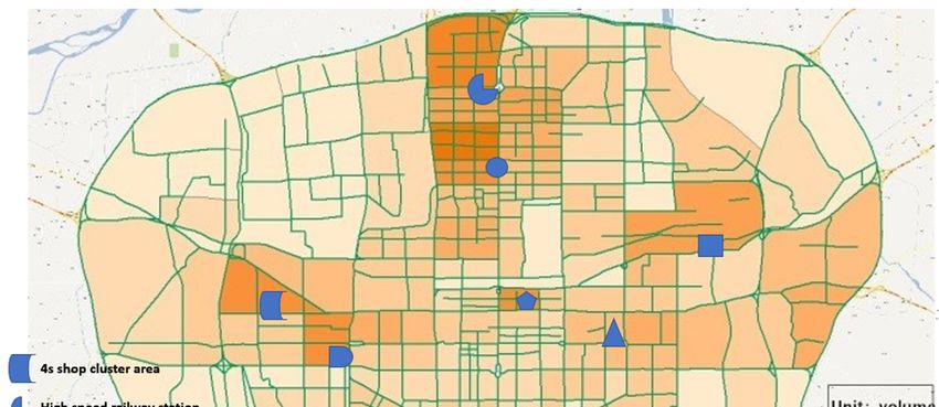
Sustainability 2019, 11, 731                                                                      3 of 19

the results should be fully considered, and the randomness and difference of the distribution of taxi
transportation demand are not considered. In the calculation process, the uniform distribution of
transport demand in the road network is usually taken as the starting point, which is prone to errors.
Additionally, those methods could not be extrapolated to larger areas, let alone nationwide application.
The complexity of the taxi industry and original data add more challenges to this problem. In addition,
these methods use historical taxi volume as input data, assuming they represent proper traffic capacity
when the legitimacy of this assumption is questioned.
      Due to the progress of mobile Internet, Internet, and other technologies, the vehicle-mounted
activity data based on individual vehicles (mainly represented by GPS data and vehicle-mounted
terminal operation data) has been widely developed and applied in the field of urban transportation
and taxi research in recent years. Ghahramani and Zhou et al. [10] proposed an exploratory spatial data
analysis algorithm based on cloud processing data analysis by cooperating with a telecom company.
The spatial analysis method was used to detect the spatial distribution of mobile phones, and the
kernel density method was used to determine these distributions. This analysis can help organizations
better implement monitoring and evaluation plans at all levels and make the necessary infrastructure
improvements to meet the needs of users. R. Tachet [11] used taxi travel data from cities such as New
York, San Francisco, Singapore, and Vienna, calculated the shareability curve of each city in the data
rather than using only some of the basic city under the premise of adjustment parameters, predicted
the carpool potential of any city under the background of the rapid development in the present city,
provided a planning engineer for the transportation company, and the society a sustainable path.
In the research of a dynamic vehicle allocation model based on dynamic data, Javier Alonso-Mora
et al. [12] studied ride-sharing services and proposed a more general real-time and large-capacity
mathematical model for ride-sharing, which could be extended to a large number of passengers
and trips, and dynamically generated optimal routes according to online requirements and vehicle
locations. The algorithm can also be used to calculate the fleet size of self-driving cars and redirect
idle vehicles to areas with high demand. Vazifeh [13] provided a web-based solution for determining
the size of a vehicle for individual travel needs. Its target is the “small vehicle fleet size operation
problem”, which is how to determine the minimum number of vehicles required for all journeys
without causing any delays to passengers. By introducing the concept of a “vehicle sharing network”,
an optimal solution of computing efficiency was proposed. This also means that in the process of
reducing urban congestion and improving the utilization rate of rental vehicles, shared travel will be
an effective measure. Paolo Santi et al. introduced the concept of a shareable network for ride-sharing
taxis, modeled the shared collective interest as a function inconvenient for passengers, and efficiently
calculated the optimal sharing strategy on a large number of data sets. Based on the data set of tens of
thousands of taxi trips in New York City, the results showed that the cumulative total travel length
can be significantly reduced under the premise of an inappropriately small increase in passengers.
The results of Paolo Santi et al. [14] showed the potential and contribution of shared taxis. Further,
Wenchao Xu and Haibo Zhou [15] studied the application of vehicle network big data in autonomous
driving technology on the basis of analyzing and processing the relationship between a network
of vehicles and big data, including vehicle geographic information. Pablo Samuel Castro et al. [16]
proposed a traffic density model building method based on the GPS data of a taxi, which can be
used to predict future traffic conditions and estimate the impact of emissions on urban air quality.
At the same time, a new method to automatically determine the traffic capacity of each section was
proposed, and its method was verified in the big data of a taxi GPS database. Zhan and Ukkusuri [17]
established a probabilistic hybrid model of urban link travel time based on the GPS data of large-scale
taxi travel in Manhattan, New York. The model regarded the taxi travel path as a potential path
and used polynomial logit distribution to model the taxi driver’s path selection behavior. Bonola
et al. [18] collected data, including its GPS from small-scale taxis in Rome over six months and made
experimental evaluations on delivery performance. The results showed that even with a relatively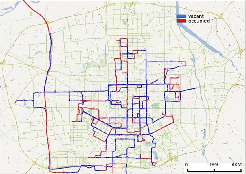
Sustainability 2019, 11, 731                                                                        4 of 19

small number of cars running in parallel in Rome, a very large and irregular city, 80% urban coverage
can be achieved in less than 24 h.
      The emerging app-based taxi service and electrical taxis raise the turnover of existing vehicles
to meet the increasing transportation demand, yet exacerbate traffic congestion. Since the operation
data from an app-based taxis are unavailable, its impact on the conventional taxi market is difficult to
quantify, decreasing the reliability and accuracy of a traditional traffic capacity calculation model. In
previous studies based on vehicles GPS big data, most of the basic data are used to study the evaluation
of urban environment, the prediction of travel time, and the service evaluation of the coverage rate of
urban areas. At present, no scholars have used the basic data information of taxi GPS to calculate taxi
fleet size and the income impact of existing operating groups.
      Based on the above research practice and progress, this paper attempts to take the typical
vehicle-mounted trajectory GPS and terminal data as the basis, under the premise of segmentation,
starting from the effective operation efficiency provided by a taxi, the total demand of residents relying
on taxi travel and the sensitivity of taxi driver’s income change. A probabilistic model of taxi-taking
based on road sections and a measurement model of the demand of unmet people are built, and a
measurement model of the taxi required fleet size is formed. Then, the income change analysis on
different transport fleet sizes is conducted through the income model. Finally, this paper takes the
on-board GPS data of taxi in Xi’an, Shaanxi Province, China in May 2014 as an example to establish
the model and verify the method.

2. Data Collection and Pre-Processing
     Xi’an is the capital of Shaanxi Province, with a total area of 10,752 square kilometers and a
population of 9,056,800. Xi’an is located at the junction of China’s land map center and two economic
regions in Central and Western China and is one of the largest node cities in the national trunk
highway network.
     This paper takes the main urban area of Xi’an City (within the ring expressway) as the case study
and takes the GPS track record of Xi’an taxis in May 2014 as the basic data for method verification
and analysis.
     Taxi GPS data uses vehicle license plate and GPS system clock as the main keys to upload
information such as the current longitude and latitude coordinates, speed value and speed direction of
the taxi as well as whether it is carrying passengers. In May 2014, Xi’an taxi track data management
system contains a total of 12,115 taxis due to vehicle maintenance, license plate replacement, suspension
and other factors. According to the statistics, the average number of vehicles in operation is 11,440,
and the amount of track data records generated is about 30 million/day. Among them, the morning
and evening peak periods (referring to relevant studies, the morning peak period in this paper is
determined as 7:00–9:00, and the evening peak period is determined as 17:00–19:00), and about 5 million
pieces of track records are recorded every day. According to the vehicle operation status reflected by
the on-off tags in the track data, the average passengers carried in the peak period are 85,083 times in
the morning peak and 81,773 times in the evening peak respectively.

2.1. GPS Trajectory Data Semantics and Travel Event Extraction
      GPS track data of a taxi is generated by vehicle terminal equipment and uploaded to data
management center by instant communication. The data content mainly includes basic information
such as vehicle license plate, driving time, driving mileage, active location (including the location
of getting on and off the vehicle) and driving speed, etc. Taking the data collected by GPS devices
of several taxis in Xi’an as an example, the trajectory data is reported at a 30-s interval, including
real-time information such as longitude and latitude (including altitude), instantaneous speed, running
direction (360 degrees), and passenger carrying status of vehicles operating on the internet. Based
on this information, more and more accurate taxi parameters can be obtained, and based on these
parameters, a more restrictive model can be established [19,20].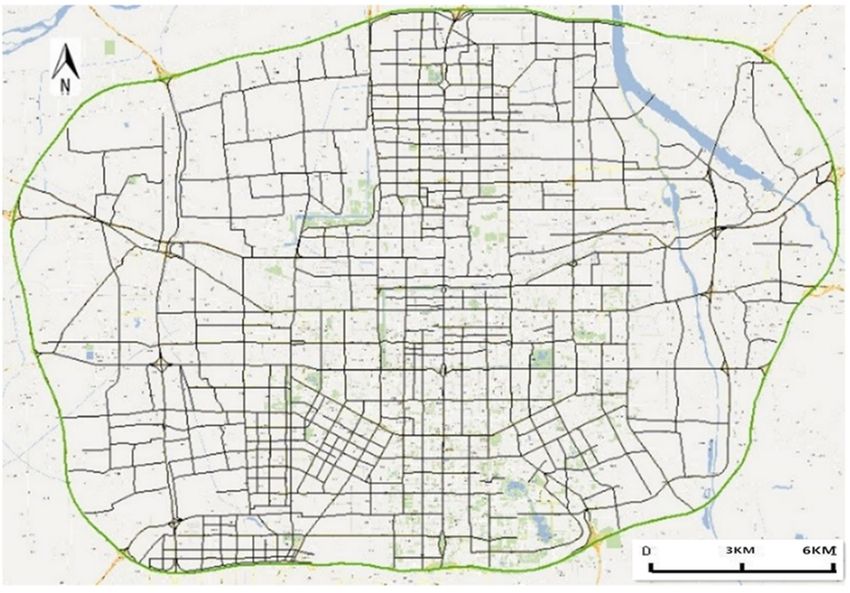
Sustainability 2019, 11, 731                                                                                        5 of 19

      The trajectory data reports the real-time information of the latitude and longitude (including
altitude), instantaneous speed, running direction (360 degrees) and passenger status of the operating
vehicle at a certain time interval. Therefore, the daily traffic activity behavior of a taxi can be considered
to be composed of multiple GPS track points, which are linearly linked in accordance with the time
series to constitute the vehicle’s driving track and reflect the information of the vehicle’s passenger
activity. Taking the data values in Table 1 as an example, the exact location of the up-down passenger
event can be considered as the two continuous points between the track state of the up-down passenger
(vehicle status from “0”→“1”) and the track state of the down-down passenger (“1”→“0”). Therefore,
the pick-up and drop-off event of a taxi can be considered as a linear event with direction and starting
and ending points from “0→1, 1→0” (Figure 1). In the figure, the solid line represents the taxi’s driving
track in the state of carrying passengers, and the dotted line represents the taxi’s driving track in the
state of vacant driving.

                                           Table 1. Research data description.

          Field                   Meaning                   Example                             Notes
   Licenseplateno       License plate number           AU1234                      Unique key
Sustainability 2019, 11 FOR PEER REVIEW                                                                     5
        in_date         Record starting time       2012/8/1 0:00:00                Unique key
      Longitude              Longitude                108.94380                   Five decimals
the time   series to constituteLatitude
       Latitude                  the vehicle’s driving34.22981
                                                        track and reflect the information    of the vehicle’s
                                                                                  Five decimals
passenger   activity. Taking the
        Height                    data values in Table 1 446
                               Altitude                   as an example, the exact location
                                                                                   No decimalof the up-down
passengerSpeed
             event can beHorizontal
                           considered speed               26
                                         as the two continuous                Unit:
                                                                 points between  thekilometer/hour
                                                                                      track state of the up-
      Direction               Direction                   90               Angle with north, clockwise
down passenger (vehicle status from “0“→ “1”) and the track state of the down-down passenger (“1
          Eff               Current status                 1                   0—invalid;1—valid
“→“0 “).Therefore, the pick-up and drop-off event of a taxi can be considered        as “1”—occupied;
                                                                           “0”—vacant;   a linear event with
       car_stat1             Car status                    1
direction and starting and ending points from “0→1, 1→0“(Figure 1). In “2”—turnedthe figure, off
                                                                                               the solid line
       car_stat3               Mileage                   1325            Cumulative  mileage,  unit: meter
represents the taxi’s driving track in the state of carrying passengers, and the dotted line represents
       car_stat4          Cumulative time           136584540000        Cumulative time, unit: millisecond
the taxi’s driving track in the state of vacant driving.

                               Figure 1.
                               Figure    Trajectory data
                                      1. Trajectory data description
                                                         description of
                                                                     of GPS
                                                                        GPS activity
                                                                            activity events.
                                                                                     events.
2.2. Trajectory Data Logic Model
                                           Table 1. Research data description.
      The linear events formed by the taxi trajectory data can be considered as the time series fed back
        Field             Meaning                         Example                              Notes
by the vehicle GPS information, which consists of a series of point sets containing time information,
                        License plate
space   information and operation information. AU1234
  Licenseplateno                                            It can be represented as a setUnique
                                                                                             {G1 ,G2 ,G
                                                                                                     key3 . . . Gm }, where
                            number
n is the total number of trajectory points formed by a taxi in a specified period of time, Gi is the locus
                                                           2012/8/1
pointin_date
       at a certain moment,
                     Record for   any Gtime
                             starting        i , we have i ∈ (1, m ). Based on the basic     composition
                                                                                           Unique    key of GPS track
                                                            0:00:00
data, according to the research needs, Gi can be designed as a one-dimensional array with six basic
    Longitude             Longitude                       108.94380                       Five decimals
items of information, Gi = {ci ,ai ,bi ,ji ,si ,vi }, where ci is the vehicle license plate, ai and bi are the longitude
      Latitude             Latitude                        34.22981                       Five decimals
and latitude values of the vehicle, si and vi are passenger carrying status and driving speed of the
       Height              Altitude                            446                         No decimal
vehicle at moment ji respectively, where si = 1 denotes occupied and si = 1 denotes vacancy.
       Speed          Horizontal speed                         26                     Unit: kilometer/hour
     Direction Information
2.3. Geographic           Direction
                             Matching                          90                 Angle with north, clockwise
          Eff          Current status                           1                      0 - invalid;1- valid
      This part mainly matches the GPS track data of taxi with the electronic map, so as to realize the
                                                                            “0”- vacant; “1“- occupied; 2“- turned
      car_stat1 betweenCar
correspondence                  status attribute of the1vehicle data and the actual geographic information.
                           the spatial
                                                                                                 off
It associates points and sections in different coordinate systems, finds the road corresponding to
      car_stat3             Mileage                           1325              Cumulative mileage, unit: meter
the vehicle’s driving track, and then determines the specific position (and driving direction) of the
      car_stat4       Cumulative time                   136584540000          Cumulative time, unit: millisecond

2.2. Trajectory Data Logic Model
     The linear events formed by the taxi trajectory data can be considered as the time series fed back
by the vehicle GPS information, which consists of a series of point sets containing time information,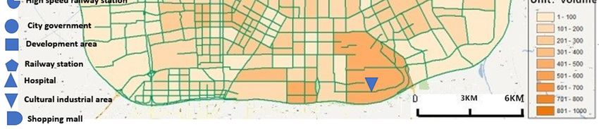
Sustainability 2019, 11, 731                                                                                     6 of 19

vehicle on a certain section of the map, so that the characteristics of vehicle travel activities and spatial
laws can be analyzed. Taking Xi’an City as an example, with the help of the electronic map of the
network (Figure 2a), based on this, the electronic map contains two parts: spatial information and
      Sustainability 2019, 11 FOR PEER REVIEW                                                                   6
attribute   information. Spatial information includes geographic location information and topological
attribute information. Spatial features are abstracted into the form of nodes, sections (lines) and traffic
      activities and spatial laws can be analyzed. Taking Xi’an City as an example, with the help of the
communities
      electronic(planes).
                    map of the network (Figure 2a), based on this, the electronic map contains two parts: spatial
      The   processand
      information       of geographic     information
                             attribute information.    matching
                                                    Spatial        method
                                                            information     usedgeographic
                                                                        includes  in this paper is asinformation
                                                                                            location  follows:
      and topological attribute information. Spatial features are abstracted into the form of nodes, sections
1.    Unified coordinate system which means that the coordinate system used to determine the vehicle
      (lines) and traffic communities (planes).
      GPSThedataprocess
                   is consistent   with the
                          of geographic      map. matching method used in this paper is as follows:
                                          information
2.    With1.the Unified
                  help of coordinate
                           ArcGIS tool    (Environmental
                                       system  which meansSystems
                                                              that the Research
                                                                       coordinateInstitute,  Inc to
                                                                                    system used  -Esri.  Redlands,
                                                                                                     determine  the CA,
      USA), the
      vehicle  GPSshortest     distancewith
                     data is consistent   method    is used to determine the road section to which GPS track
                                              the map.
     points2. belong.
                 With the help of ArcGIS tool (Environmental Systems Research Institute, Inc -Esri.
3.    Redlands,
      Match theCA,      USA), the
                     direction      shortest distance
                                information    of roadmethod
                                                        segment is used
                                                                   withtothe determine
                                                                               directionthe road sectionoftotrack
                                                                                          information        whichpoint,
      GPS track points belong.
      determine the direction of vehicle travel. Classify the track points and the information, such as
           3. Match the direction information of road segment with the direction information of track
      speed, is imported into the spatial attribute database
      point, determine the direction of vehicle travel. Classify the track points and the information, such as
      speed,
     In       is imported
          practical         into the this
                       operation,    spatial attribute
                                            paper  usesdatabase
                                                          Xi’an-1980 plane coordinate and WGS-1984 earth
           In practical operation, this paper uses Xi’an-1980 plane coordinate and WGS-1984 earth
coordinates are adopted in this paper for GPS track data. In order to ensure the consistency of
      coordinates are adopted in this paper for GPS track data. In order to ensure the consistency of the
the coordinate system, coordinate transformation is realized through ArcGIS. The result of map
      coordinate system, coordinate transformation is realized through ArcGIS. The result of map
matching    is shown
      matching          in Figure
                  is shown          2b 2b
                             in Figure  and  vehicle
                                           and vehicletrack
                                                       trackrestoration
                                                             restoration isisshown
                                                                              showninin  Figure
                                                                                       Figure 2c.2c.

                                              (a) Road network extraction.

                                                (b) Trajectory matching.

                                                   Figure 2. Cont.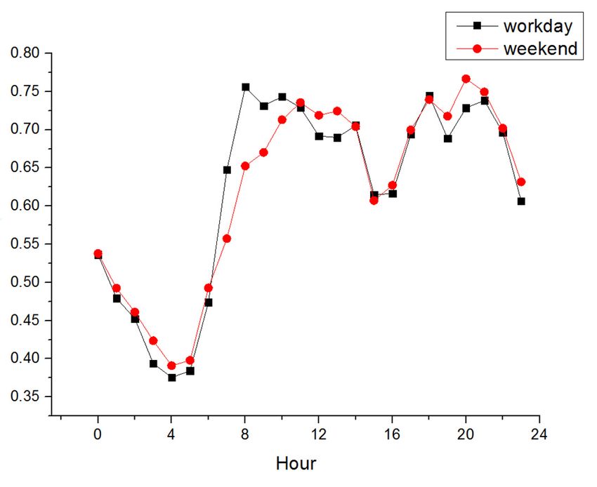
Sustainability 2019, 11, 731 7 of 19
Sustainability 2019, 11 FOR PEER REVIEW 7
(c) Vehicle track restoration (one vehicle demonstration).
Figure 2.
Figure Road network
2. Road network extraction,
extraction, trajectory
trajectory matching,
matching, and
and vehicle
vehicle track
track restoration.
restoration.
3. Methodology
3. Methodology
3.1. Ideas and Assumptions
3.1. Ideas and Assumptions
As a kind of urban traffic supply, it should be the fundamental starting point to consider the
As
reasonablea kindfleetofsize
urbanfrom traffic supply, it should
the perspective be the
of solving the fundamental
difference betweenstarting point supplytoand consider
demand. the
reasonable fleet size from the perspective of solving the difference
However, it should be noted that many factors, such as the effectiveness of urban road network, between supply and demand.
However, it should
the development be noted
degree that many
of public factors, such
transportation, theasoperating
the effectiveness
efficiency of ofurban
a taxi road network,time
(including the
development degree of
efficiency and mileage public transportation,
efficiency), the operating
the spatial distribution efficiency
of taxi travel, and the of apricetaxiof(including
a taxi will havetime
efficiency and mileage efficiency), the spatial distribution of taxi travel,
an impact on the demand scale of a taxi [21]. In addition, different modes of taxi hiring have different and the price of a taxi will
have an impact
efficiencies on thedemands.
of meeting demand scale of a taxi [21].
An important pointInisaddition, different
that the travel demand modes of of taxiishiring
a taxi have
essentially
different efficiencies of meeting demands. An important point is that the
reflected in the time and space of one or more areas “in short supply (difficult to take a taxi)”, such as travel demand of a taxi is
essentially reflected in the time and space of one or more areas “in
the peak hours in some hot areas. However, in a flat hump period, even in some remote areas (areas short supply (difficult to take a
taxi)”,
that aresuch
not as the peak
easily hoursorinnot
accessible some hot areas.
willing However,
to be reached byin a flattaxis
taxi), hump areperiod,
actuallyeven not in in some remote
short supply;
areas (areas that are not easily accessible or not willing to be reached
in essence, it can be understood as a scheduling problem. That is, when the fleet size is sufficient, by taxi), taxis are actually not
in short supply; in essence, it can be understood as a scheduling problem.
the subproblems can be solved through reasonable operation scheduling. Therefore, this situation is That is, when the fleet size
is
notsufficient,
within the the subproblems
scope can be
of this article. Insolved through
conclusion, the reasonable
reasonable operation
fleet size ofscheduling.
taxi shouldTherefore,
be carried this out
situation is not within the scope of this article. In conclusion,
under certain assumptions. The assumptions set in this paper are as follows: the reasonable fleet size of taxi should
be carried out under certain assumptions. The assumptions set in this paper are as follows:
1. 1. DuringDuringa research period,
a research residents’
period, travel habits
residents’ travel remain
habits unchanged,
remain unchanged, and thereand is nothere
significant
is no
change
significant in theinurban
change the urbancomprehensive
comprehensive transportation
transportation system
system (rail
(rail transit
transitisisnewly
newly built, etc.).
built, etc.).
The overall number of taxi trips is stable; that is, in other words,
The overall number of taxi trips is stable; that is, in other words, the number of taxi rides is generally the number of taxi rides is
generally stable.
stable.
2. 2. The The
operating
operatingpriceprice
of taxi andand
of taxi other operating
other operating prices are are
prices stable, which
stable, whichmeans means there willwill
there be no
be
transfer
no transfer oror change
change ofof
thethe traveling
traveling population
population caused
caused byby economic
economic factors.
factors.
3. 3. The The research
research object object of this
of this paperpaper
is theis the number
number of times
of times to take
to take a taxi,
a taxi, rather
rather thanthan thethe number
number of
of people
people to take
to take a taxi, which
a taxi, whichmeans oneone
means person
personor more
or more taking a taxi
taking together
a taxi togetheris considered
is considered as one as
time. one time.
4. 4. The The
fleet fleet size isthat
size that is needed
needed to be added
to be added in thisin this paper’s
paper’s discussion,
discussion, is the amount
is the amount of fleet
of fleet needed
neededforfor
unmetunmet demand
demand on on these
these “not“not supply
supply (hard(hard to take
to take a taxi)”
a taxi)” road road sections
sections or areas
or areas duringduringthe
the peak
peakhours.
hours.As Asexplained
explainedin in the
the previous paragraph,
paragraph,the theproblem
problemofof“difficulty
“difficultyinin taking
taking a taxi”
a taxi” in
in remote areas is not considered as a real lack of demand, so it is not within
remote areas is not considered as a real lack of demand, so it is not within the scope of this paper. the scope of this paper.
5. 5. Allcar-hailing
All the the car-hailing modes modes involved
involved in thisinpaper
this paper
followfollow the principle
the principle of “firstofcome, “firstfirst
come, first
served”
served” and do not consider the taxi’s no-load behavior when driving
and do not consider the taxi’s no-load behavior when driving vacant; that is, if a “vacant car” vacant; that is, if a “vacant car”
passes a road section without stopping to pick up a passenger, then the road section is deemed to
have no demand.
Sustainability 2019, 11, 731                                                                           8 of 19

       passes a road section without stopping to pick up a passenger, then the road section is deemed to
       have no demand.
6.     The service form of the taxi in this paper is traditional taxi service, which does not consider the
       use of telephone or network for lease, because this situation will make the five-hypothesis invalid.

      Based on the above assumptions, this paper takes the average effective mileage provided by a
taxi and the total demand for taxi travel in the city as the core research objects, discusses taxis under
the constraint of considering the change threshold of the taxi driver’s income change, and looks at the
relationship between the fleet size of the taxi and the total passengers transport volume when the taxi
fleet size meets the transportation demand. Steps are as follows:

1.     Divide the roads network into multiple section units, on which the passengers’ taxi-hailing
       actions were abstracted into a queuing problem, based on the random process theory to build the
       probability model of taxi [22]. Through calculating the difficulty degree of taking a taxi for each
       road section, find out the road sections with “short supply (difficult to take a taxi)”. These road
       sections are called “difficult to take a taxi areas”.
2.     Calculate the unmet demand for taxi according to queuing theory.
3.     Based on the track data, the operating efficiency of taxis in different time ranges is calculated to
       seek the effective operating efficiency provided by taxis in peak hours
4.     Through the unmet total demand and the taxi operating efficiency, seek the reasonable size range
       of taxi fleet demand.
5.     Calculate the change of taxi driver’s income under different fleet demand scale, or under the
       influence of different income, the taxi driver’s fleet size.

3.2. Taxi Operation Index

3.2.1. Mileage Utilization
      The mileage utilization rate of taxi refers to the percentage of passenger miles in the total mileage
during the operating period of the taxi, which can reflect the operating status of taxi more intuitively.
The average mileage utilization rate of the overall taxis a city can reflect, to some extent, whether taxi
fleet size in a city is reasonable; the lower the mileage utilization rate is, the greater the invalid traffic
flow caused by taxis in the urban road network and excess taxi fleet scale will be. Mileage utilization is
calculated as follows:
      The average operating mileage can be expressed as:

                                                    ∑ gij
                                            gz =            t2 ∈ T                                        (1)
                                                     N
where t2 donates unit time, T is the time range (can be taken in 24 h or taken in unit time), gz denotes
the average operating mileage in the time range of T, N denotes total amount of the taxi fleet size,
i denotes the ith taxi, j denotes that the taxi is in state j, where j = 1 denotes carrying passengers and
j = 0 denotes vacant driving.
      The average passenger mileage can be expressed as:

                                                    ∑ gi1
                                            gz0 =            t∈T                                          (2)
                                                     N

where g0 z donates the average passenger mileage in the time range of T.
    Mileage utilization can be expressed as:
                                                     gz
                                              K=            t∈T                                           (3)
                                                     gz0

where K donates the mileage utilization in the time range T.
Sustainability 2019, 11, 731 9 of 19
3.2.2. Time Utilization
The time utilization rate of taxi refers to the percentage of the passenger carrying time in the total
working time during the operating period of the taxi, which can reflect the relationship between the
working time and efficiency of taxi drivers intuitively. The working hours of taxi drivers, on the one
hand, reflects the time characteristics of urban residents who rely on taxis for travel. On the other
hand, the time utilization rate can reflect whether the taxi fleet size in this city is reasonable to some
extent; the lower the time utilization rate is, the less the effective working hours are and the higher the
surplus of the fleet size is. Time utilization is calculated as follows:
The average working time can be expressed as:
∑ tij
tg = (4)
N
where tg donates the average working time.
Average passenger carrying time can be expressed as:
∑ ti1
tc = (5)
N
where tc donates the average passenger carrying time.
Time utilization can be expressed as:
tg
K= t∈T (6)
tc
3.3. Taxi-Hailing Probability Model
Passengers may need taxi service in any segments of the urban road network, and the demand
was met randomly by any vacant taxi available on-site. With collected data, taxi utilization status and
the average time utilization rate in any given segment could be calculated to represent the operation
efficiency. The taxi arrival could be considered as a random “birth-and-death” process according to the
random theory. Poisson process was assumed, and the taxi arrival probability was presented as:
(λx )k − λx
pk = e (7)
k!
where pk denotes the probability that k taxis would arrive in x time span, λ denotes the average interval
between two consecutive taxis, and x denotes the numerical time interval.
Average taxi arrival in high demand segments could be calculated with tracking data:
∑ ni
λ= (8)
t
where t denotes research time span, ni denotes the number of taxis arriving in i status, i = 1 means the
taxi was occupied, and i = 0 means the taxi was vacant.
The probability of getting a taxi could be simplified according to the Taylor formula:
n1 + n2
p = 1 − e− t p (1− o )
(9)
where p represents numerical time interval i.e., passenger waiting time, ni denotes the number of
taxis arriving in i status, t denotes the research time span, o denotes time utilization rate, i.e., the ratio
between carrying time and total operation time, i = 1 meant the taxi was occupied, and i = 0 meant the
taxi was vacant.Sustainability 2019, 11, 731 10 of 19
The above model reflected the probability for a passenger to get taxi service in a given waiting
time. The criteria to qualify the difficulty to get taxi service was defined subjectively. In this study, for
example, the probability that a passenger can get a taxi in five minutes on a certain road section is 95%,
or the probability that a passenger can get a taxi in 10 min on a certain road section is 50%. When the
model is calculated, the standard to measure the difficulty of taking a taxi should be set according to
the actual situation. If the probability of getting taxi service in 10 min is less than 75%, that segment
would be labeled as a segment with low taxi availability.
3.4. Total Taxi Service Mileage Calculation Model
In each study road section, when the arrival rate of taxi passengers is higher than that of vacant
cars, based on the random theory, the taxi service process can be regarded as a random birth and
death process, abstracting into a queuing problem. Many researchers have agreed on viewing the
taxi service as a random “birth-and-death” process from random process [23], driver route selection
experience [24], and other perspectives. Assuming passengers arrive in Poisson flow with parameter
λ, when there is no available taxi they start waiting and would shift to other options if the waiting
time reaches a threshold and become missed taxi customers. Assume that the queuing passengers
give up following a Poisson distribution with strength 4k and the service time of vacant taxis in the
given segment obeyed negative exponential distribution with parameter µ. When 4k = kδ, δ > 0,
the following equation was used to calculate the probability when the number of waiting passengers
in a given segment was k. When k = 1:
λp0 = µp1 (10)
When k = 2:
λ2 p2 δ
p2 = p0 = p0 ( β + ) (11)
µ(u + δ) 1+β µ
where λ is the passenger arrival parameter, i.e., the passenger arrival rate, and µ was service time
parameter, i.e., the vacant taxi arrival rate in unit time in a given segment. λ could be obtained through
survey or calculated with equation. Assume that average waiting time is known, and all passengers
are transported, then the passenger arrival rate would be:
µ2 τε
λ= (12)
µ2 τε+1
where τε denotes the average waiting time.
Then the probability when k passengers were waiting in a given segment could be represented as:
p k p0
pk = (13)
(1 + β) + (1 + 2β)....[1 + (k − 1) β]
where ρ denotes the system load level or intensity, ρ = λ/µ.
Average system queue length could be presented as:
n n
kpk ρ
ms = ∑ kpk < ∑ (k − 1)!βk−1 p0 = ρ(1 − β ) p0 eρ/β (14)
k =0 k =1
In a nutshell, the average system queue length is the function of waiting time and vacant car
arrival rate. Numerically, it equals to taxi trips required to satisfy the unmet demand within a given
waiting time. The unmet transportation turnover could be calculated via multiplying it with average
trip distance. Total taxi service mileage refers to the total carrying kilometers covered by taxis when
all the transportation demand is met within a given waiting time. When the taxi-hailing probability
calculated with the above model is within a receptible range in all segments, the traffic capacitySustainability 2019, 11, 731 11 of 19
is considered to be sufficient. Otherwise, unmet demand exists, and the required total mileage is
represented as:
wt = w a + wn t ∈ T, (15)
where w denotes the required total taxi mileage within time span t, wa denotes the finished taxi mileage
within time span t, and wn denotes the unmet taxi mileage within time span t.
The unmet taxi mileage within time span t could be represented as the sum of the unmet taxi trip
distance in all segments with low taxi availability in the urban road network:
n n
wn = ∑ wi = ∑ m i l i (16)
i =1 i =1
where wn denotes the unmet taxi mileage within time span t, wi denotes the unmet taxi mileage in the
i segment, mi denotes the unmet taxi requests in the i segment, i.e., the missed trips, and l i denotes the
average trip distance in the i segment.
It is inevitable that the taxi will generate invalid mileage during the cruise, due to the difference
of taxi transportation demand in different time periods and the decrease of taxi running speed caused
by urban congestion. There are obvious differences in the mileage utilization rate of taxi, therefore,
the operating efficiency of taxis in different time periods is affected by the speed and the online rate
of vehicles (the ratio of the number of vehicles put into operation in unit time to the total number).
According to the definition of mileage utilization, it can be expressed as:
nt
h0t = uht = uK ∑ qi t∈T (17)
i =1
0
where u is taxi mileage utilization (%), ht is the sum of the effective mileage of all taxis operating
within a unit of time (km), ht is the total number of miles driven by all operating taxis per unit of time
(km), nt is the fleet size of taxi put into operation within the time range of t (unit), T is the time range,
unit operation time, i is the ith taxi, and qi is the mileage of the ith taxi in the time range of t.
The average effective mileage supplied by a taxi cycle in the time range t can be expressed as:
nt
u ∑ qi
i =1
h0a = (18)
nt
where ha 0 donates the average effective mileage supplied by a taxi cycle in the time range t (km), and
nt is the fleet size of taxi put into operation within the time range of t (unit).
3.5. Taxi Fleet Size Adjustment Model
Above all, the incremental taxi volume required in a period could be calculated [24]:
wn
χ=ϕ (19)
L0a
where ϕ denotes the satisfactory degree coefficient varying between 0 and 1, wn denotes the unmet
urban taxi passenger transportation turnover in an hour, and L0a denotes the average taxi effective
mileage in unit time.
Incremental taxi volume needed to satisfy unmet demand in each hour could be calculated with
the volume model. The final number should lie within the range defined by the value in peak hours
and that in off-peak hours, which is approximately zero. Therefore, the total incremental taxi volume
was calculated as follows:
x ∗ = ∂1 x1 , ∂2 x2 , · · · ∂ n x j
(20)the volume model. The final number should lie within the range defined by the value in peak hours
and that in off-peak hours, which is approximately zero. Therefore, the total incremental taxi volume
was calculated as follows:
x * ={ ∂1 x1 , ∂ 2 x2 , ∂ n x j } (20)
Sustainability 2019, 11, 731 12 of 19
where x* denotes the final incremental capacity, ∂ denotes the satisfactory degree coefficient
* denotes the final incremental capacity, ∂ denotes the satisfactory degree coefficient varying
varyingx between
where 0 and 1, and xj denotes the incremental capacity in each of the time unit within 24
hours. 0 and 1, and xj denotes the incremental capacity in each of the time unit within 24 h.
between
3.6. Taxi Market Supply-Demand Mechanism and Income Constraint Model
3.6. Taxi Market Supply-Demand Mechanism and Income Constraint Model
The above method was built upon the assumption that both the taxi industry and resident
The above method was built upon the assumption that both the taxi industry and resident
transportation demand would remain stable. The basic concept was to mitigate the difficulty of
transportation demand would remain stable. The basic concept was to mitigate the difficulty of
getting taxi service during the times where taxi demand is high. Demand for a taxi is difficult to
getting taxi service during the times where taxi demand is high. Demand for a taxi is difficult to
quantify, but could be reflected by the deadhead rate, which is correlated to operation cost, operation
quantify, but could be reflected by the deadhead rate, which is correlated to operation cost, operation
efficiency, and average waiting time. The vacancy rate reflects the degree of passengers’ demand for
efficiency, and average waiting time. The vacancy rate reflects the degree of passengers’ demand for
taxis from a certain perspective. The smaller the vacancy rate is, the greater the passengers’ demand
taxis from a certain perspective. The smaller the vacancy rate is, the greater the passengers’ demand
will be. [25–28]. Similarly, the operational effectiveness is also related to the vacancy rate. Under the
will be. [25–28]. Similarly, the operational effectiveness is also related to the vacancy rate. Under the
condition of constant input quantity and freight rate, the higher the vacancy rate is, the greater the
condition of constant input quantity and freight rate, the higher the vacancy rate is, the greater the
waste of resources will be and the smaller the operating profit will be. As a result of the launch of new
waste of resources will be and the smaller the operating profit will be. As a result of the launch of
transport capacity, passengers’ waiting time will be reduced, and residents’ travel choices will change.
new transport capacity, passengers’ waiting time will be reduced, and residents’ travel choices will
Accordingly, the number of trips completed by taxis will increase, and the transportation demand
change. Accordingly, the number of trips completed by taxis will increase, and the transportation
will increase. Therefore, the supply and demand mechanism of the taxi market has been in dynamic
demand will increase. Therefore, the supply and demand mechanism of the taxi market has been in
change,
dynamicaschange,
illustrated in Figure in
as illustrated 3. Figure 3.
Figure 3. Supply and demand dynamic in the taxi market.
Considering
Considering the
the dynamics
dynamics andand complexity
complexity of of the
the supply
supply and demand balance
and demand balance mechanism
mechanism of of the
the
taxi,
taxi, after
after the
the delivery of transport
delivery of transport capacity,
capacity, it
it reaches
reaches aa new
new steady
steady state
state rather
rather than
than anan equilibrium
equilibrium
state,
state, which
which can
can be
be observed
observed according
according to
to the
the calculation
calculation model.
model. When
When the
the stability
stability is
is reached
reached again
again
and the waiting time exceeds the threshold, the delivery can continue. The delivery of
and the waiting time exceeds the threshold, the delivery can continue. The delivery of taxis alsotaxis also needs
needs
to
to comply
comply withwith the
the laws
laws ofof the
the market
market and
and constrain
constrain the
the delivery
delivery of
of capacity
capacity through
through changes
changes inin
income:
income: t
∑ ci
cu it=1
ε = 1− = 1− (21)
co
cu ∑ cj
t0 c
i
ε = 1− = 1− i =1
j =1
t' (21)
co
where ε denotes the income variation index ranging between
c j 0 and 1, co denotes the average income
j =1 volume increase, c denotes the average
before volume increase, cu denotes the average income after j
income at j hour before volume increase, ci denotes the average income at i hour after volume increase,
t0 denotes average working hours before volume increase, and t denotes the average working hours
after volume increase.
4. Results and Discussion
4.1. Analysis on the Taxi Operation Characteristics
According to Equations (1)–(3), the average daily mileage utilization rate of taxis in Xi’an is 66%,
and the mileage utilization rate in morning and evening peak hours is 76% and 75%, respectively.average working hours after volume increase.
4. Results and Discussion
4.1. Analysis on the Taxi Operation Characteristics
Sustainability 2019, 11, 731 13 of 19
According to Equations (1)–(3), the average daily mileage utilization rate of taxis in Xi’an is 66%,
and the mileage utilization rate in morning and evening peak hours is 76% and 75%, respectively.
The distribution
The distribution ofof weekdays
weekdays and and non-weekdays
non-weekdays is is shown
shown in in Figure
Figure 4. 4. The
The overall
overall trend
trend in
in mileage
mileage
utilization shows
utilization shows two
two low
low peaks,
peaks, which
which are
are 3:00–4:00
3:00–4:00 and
and 15:00–16:00.
15:00–16:00. Compared with the first peak,
the mileage
the mileage utilization
utilization ratio
ratio of
of rest
rest days
days andand weekdays
weekdays presents a certain certain degree of “dislocation”
phenomenon,the
phenomenon, thefirst
firstpeak
peakofofthe
theweekdays
weekdaysoccurs
occursatat 8:00,
8:00, andand
thethe first
first peak
peak of of
thethe
restrest days
days occurs
occurs at
at 11:00,
11:00, andand
thethe
peakpeakof of
thethe rest
rest days
days mileage
mileage utilizationlags
utilization lagsbehind
behindthe theweekdays,
weekdays,the thesecond
second peak
peak
of weekdays
of weekdays and and rest
rest days
days overlaps
overlaps at at 18:00
18:00and
andremained
remainedstable
stableatat22:00.
22:00. Overall,
Overall, thethe utilization
utilization
efficiencystill
efficiency stillhas
hasaa high
high mileage
mileage utilization
utilizationrate
rateeven
even atat night,
night, which
which is is directly
directly related
related to
to the
the number
number
of passengers
of passengers and
andthe thenumber
numberof ofoperating
operatingtaxis,
taxis,as
asshown
shownin inFigure
Figure4.4.
Figure 4. Interval
Figure 4. Interval distribution
distribution of
of the
the mileage
mileage utilization
utilization rate.
rate.
According to Equations (4)–(6), the calculation results show that the utilization rate of morning
According to Equations (4)–(6), the calculation results show that the utilization rate of morning
and evening peak hours in Xi’an are 76% and 75%, respectively. At the same time, there is a strong
and evening peak hours in Xi’an are 76% and 75%, respectively. At the same time, there is a strong
correlation between mileage utilization rate and time utilization rate, the correlation coefficients are
correlation between mileage utilization rate and time utilization rate, the correlation coefficients are
all over 0.95, and the trend of time utilization efficiency and mileage utilization efficiency is basically
all over 0.95, and the trend of time utilization efficiency and mileage utilization efficiency is basically
consistent. According to the survey results of residents’ travel in Xi’an in 2008, the trend of the time
consistent. According to the survey results of residents’ travel in Xi’an in 2008, the trend of the time
utilization rate of taxis on weekdays is basically consistent with the distribution of residents’ travel
utilization rate of taxis on weekdays is basically consistent with the distribution of residents’ travel
time. The two peak periods are the commuting peak of urban residents respectively, and these two
time. The two peak periods are the commuting peak of urban residents respectively, and these two
trips account for about 25% of the total travel volume of residents, as shown in Figure 5.
trips account for about 25% of the total travel volume of residents, as shown in Figure 5.Sustainability 2019, 11, 731 14 of 19
Sustainability 2019, 11 FOR PEER REVIEW 14
Sustainability 2019, 11 FOR PEER REVIEW 14
rate.
Figure 5. Interval distribution of the time utilization rate.
Figure 5. Interval distribution of the time utilization rate.
4.2.
4.2. Taxi
Taxi Operation
Operation Space
Space Characteristics
Characteristics
4.2. Taxi Operation Space Characteristics
In
In this
this paper,
paper, the
the regional
regional taxi
taxi demand
demand scale
scale based
based onon the
the division
division of of the
the community
community is is used
used to
to
In this
illustrate paper,
the the regional
characteristics taxi
of thedemand
taxi scale
operationbased on
space, the
a division
total of 201 of the
traffic community
communities
illustrate the characteristics of the taxi operation space, a total of 201 traffic communities are divided is used
are to
divided in
illustrate
Xi’an the characteristics
within three ringringof theThe
roads. taxiArcGIS
operation space,
spatial a total tool
analysis of 201 traffic communities are divided
in Xi’an within three roads. The ArcGIS spatial analysis is used
tool to
is used study the changes
to study of hotof
the changes spots
hot
in where
Xi’an within three
residents ring
use roads.
taxis to The
travel ArcGIS
at any spatial
time. analysis
The tool
comparison is used
of to
gettingstudyon the
the changes
taxis in of hot
morning and
spots where residents use taxis to travel at any time. The comparison of getting on the taxis in
spots where residents
evening use taxis to travel at any time. The comparison ofingetting on actually
the taxismeans
in
morningpeak and hours
eveningof Xi’an
peak city
hoursis shown below
of Xi’an city as
is Figure
shown 6.below
Volumeas Figurethe maps
6. Volume the
in the maps
morning and
taxi-taking evening
times. peak hours of Xi’an city is shown below as Figure 6. Volume in the maps
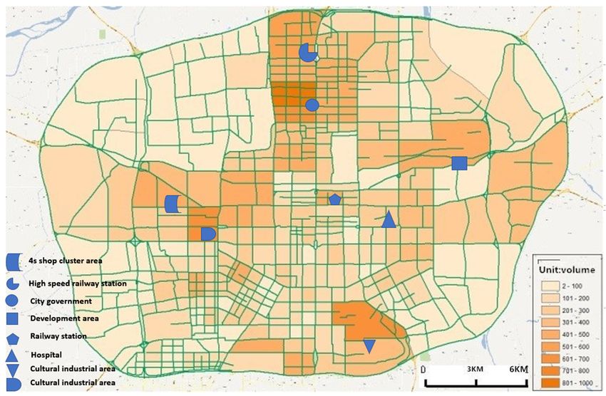
actually means the taxi-taking times.
actually means the taxi-taking times.
(a) Morning peak hours.
(a) Morning peak hours.
Figure 6. Cont.Sustainability 2019, 11, 731 15 of 19
Sustainability 2019, 11 FOR PEER REVIEW 15
(b) Evening peak hours.
Figure 6. Traffic
Figure6. Traffic zone’s pick-up
pick-upvolume
volumedistribution
distributionininpeak
peak hours.
hours.
The
Theresults
resultsshow
showthat
that the
the regions with high
regions with high demand
demandfrequency
frequencyininthethe Xi’an
Xi’an taxi
taxi network
network areare
located
locatedininthe
thenorth,
north, west, southeast,and
west, southeast, andnortheast,
northeast, respectively.
respectively. During
During peakpeak hours,
hours, the amount
the amount of
oftaxi
taxirides
ridesininhothotspots
spotstotaled
totalednearly
nearly3000
3000times.
times.After
After
map matching, it can be seen that thethe
map matching, it can be seen that
geographic
geographiclocations
locationscorresponding
corresponding to to the
the four
four regions
regionsare
arethe
themunicipal
municipalgovernment,
government, municipal
municipal
library,
library, largesupermarket,
large supermarket,shopping
shopping mall, office
office building,
building,hospital,
hospital,railway
railwaystation, and
station, other
and major
other major
functional sites in cities, which are basically consistent with the actual situation, where
functional sites in cities, which are basically consistent with the actual situation, where these “hot these “hot
spots”are
spots” arethe
thefocus
focusofofthis
thispaper.
paper.
4.3.Fleet
4.3. FleetSize
SizeCalculation
Calculationand
andAdjustment
Adjustment
Accordingtotothe
According thetaxi
taxiprobability
probabilitymodel,
model,totocalculate
calculatethe
thetaxi
taxiprobability
probabilityofofeach
eachsection,
section,due
due to
tothe
the subjective differences in the degree of difficulty in taxi taking between different
subjective differences in the degree of difficulty in taxi taking between different regions and different regions and
different
groups. In groups. In this
this study, study,
if the if the probability
probability of a passenger
of a passenger getting agetting a taxi five
taxi within within five minutes
minutes of
of a section
is aless
section
thanis75%,
less than
it is 75%, it is considered
considered as a “taxiasdifficult”
a “taxi difficult”
section.section. Bringing
Bringing the data
the taxi taxi data
into into the
the above
above calculations indicates that there are road sections that are difficult to travel in multiple time
calculations indicates that there are road sections that are difficult to travel in multiple time frames,
frames, and it is necessary to increase the fleet size to meet the transportation needs.
and it is necessary to increase the fleet size to meet the transportation needs.
Withthethe
With available
available datadataandandthe the
aboveabove methodology,
methodology, let value
let the the value
of ∂ beof1, ∂andbethe1, incremental
and the
incremental taxi volume in Xi’an to completely satisfy transportation demand
taxi volume in Xi’an to completely satisfy transportation demand for each hour from 8:00–13:00 for each hour from 8and
:00–13:00
from and from
17:00–22:00 was17:00–22:00
calculatedwas andcalculated
shown in and
Tableshown
2. in Table 2.
The results show that the required incremental volume ranged between 654 and 2237 taxis, with
Table 2. Incremental taxi volume in specific hours.
the requirement for peak hours significantly higher than that for off-peak hours. In practice, an increase
in accordance to the maximum Time1 demand would result 8:00 in excessive
9:00 10:00 11:00in 12:00
capacity off-peak 13:00
hours.
Current Mileage Utilization Rate (%) 0.76 0.73 0.74 0.73 0.69 0.69
Current Speed (km/h) 22.86 22.81 22.36 23.81 26.80 26.31
Calculated Incremental Volume (cars) 2150 2022 1126 824 658 784
Time 17:00 18:00 19:00 20:00 21:00 22:00
Current Mileage Utilization Rate (%) 0.69 0.74 0.69 0.73 0.74 0.70You can also read


