Time Series Forecasting Principles with Amazon Forecast - Technical Guide - Awsstatic
←
→
Page content transcription
If your browser does not render page correctly, please read the page content below
Time Series Forecasting
Principles with Amazon Forecast
Technical Guide

February 2020
Notices
Customers are responsible for making their own independent assessment of the
information in this document. This document: (a) is for informational purposes only, (b)
represents current AWS product offerings and practices, which are subject to change
without notice, and (c) does not create any commitments or assurances from AWS and
its affiliates, suppliers or licensors. AWS products or services are provided “as is”
without warranties, representations, or conditions of any kind, whether expressed or
implied. The responsibilities and liabilities of AWS to its customers are controlled by
AWS agreements, and this document is not part of, nor does it modify, any agreement
between AWS and its customers.

© 2020 Amazon Web Services, Inc. or its affiliates. All rights reserved.
Contents
Overview ..............................................................................................................................1
About Forecasting ...............................................................................................................1
   Forecasting System .........................................................................................................2
   Where Do Forecasting Problems Occur?........................................................................2
   Considerations Before Attempting to Solve a Forecasting Problem ..............................3
Case Study: Retail Demand Forecasting Problem for an E-Commerce Business............4
Step 1: Collect and Aggregate Data ...................................................................................6
Step 2. Prepare Data ...........................................................................................................9
   How to Handle Missing Data ...........................................................................................9
   Concepts of Featurization and Related Time Series ....................................................11
Step 3: Choose a Model ....................................................................................................13
Step 4: Evaluate Forecasts ...............................................................................................14
   Backtesting .....................................................................................................................15
   Quantile Losses and Probabilistic Forecasts ................................................................17
   Problems with MAPE and RMSE...................................................................................19
Step 5: Generate Forecasts and Use Forecasts for Decision Making.............................20
   Visualization ...................................................................................................................20
Summary of Forecasting Workflow and APIs ...................................................................21
   Using Amazon Forecast for Common Scenarios ..........................................................22
   Implementing Forecast into Production .........................................................................23
Conclusion .........................................................................................................................23
Contributors .......................................................................................................................24
Further Reading .................................................................................................................24
Document Revisions..........................................................................................................25
Appendix A: FAQs .............................................................................................................26
Appendix B: References....................................................................................................27

About this Guide
Companies today use everything from simple spreadsheets to complex financial
planning software in a bid to accurately forecast future business outcomes such as
product demand, resource needs, and financial performance. This paper introduces
forecasting, its terminology, challenges, and use cases. This document uses a case
study to reinforce forecasting concepts, forecasting steps, and references how Amazon
Forecast can help solve the many practical challenges in real-world forecasting
problems.
Amazon Web Services                      Time Series Forecasting Principles with Amazon Forecast

Overview
Forecasting is the science of predicting the future. By using data historical data,
businesses can understand trends, make a call on what might happen and when, and in
turn, build that information into their future plans for everything from product demand to
inventory planning and staffing.

Given the consequences of forecasting, accuracy matters. If a forecast is too high,
customers may over-invest in products and staff, which results in wasted investment. If
the forecast is too low, customers may under-invest, which leads to a shortfall in raw
materials and inventory; creating a poor customer experience.

Today, businesses try to use everything from simple spreadsheets to complex
demand/financial planning software to generate forecasts, but high accuracy remains
elusive for two reasons. First, traditional forecasts struggle to incorporate large volumes
of historical data, missing important signals from the past that are lost in the noise.
Second, traditional forecasts rarely incorporate related but independent data, which can
offer important context (such as sales, holidays/events, locations, marketing
promotions, etc.). Without the full history and the broader context, most forecasts fail to
predict the future accurately.

Amazon Forecast is a fully managed service that overcomes these problems. Amazon
Forecast provides the best algorithms for the forecasting scenario at hand. In particular,
it relies on modern machine learning and deep learning, when appropriate to deliver
highly accurate forecasts. Amazon Forecast is easy to use and requires no machine
learning experience. The service automatically provides the necessary infrastructure,
processes data, and builds custom/private machine learning models that are hosted on
AWS and ready to make predictions. In addition, as advances in machine learning
techniques continue to evolve at a rapid pace, Amazon Forecast incorporates these, so
that customers continue to see accuracy improvements with minimal to no additional
effort on their part.

About Forecasting
In this document, forecasting means predicting the future values of a time series: the
input or output to a problem is of a time series nature.

                                                                                              1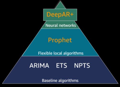
Amazon Web Services Time Series Forecasting Principles with Amazon Forecast
Forecasting System
A forecasting system includes a diverse set of users:
• End users, who query the forecast for a specific product, and decide how many
units to purchase; this may be a person or an automated system.
• Business analysts/business intelligence, who support end users, run and
organize aggregate reporting.
• Data scientists, who iteratively analyze the demand patterns, causal effects,
and add new features to deliver incremental improvements to the model or
improve the forecasting model.
• Engineers, who set up the infrastructure of the data collection, and ensure the
availability of the input data to the system.
Amazon Forecast alleviates the work of software engineers and allows businesses with
limited data science capabilities to leverage state of the art forecasting technology. For
businesses with data science capabilities, a number of diagnostic functionalities are
included so that forecasting problems are well addressed with Amazon Forecast.
Where Do Forecasting Problems Occur?
Forecasting problems occur in many of the areas which naturally produce time series
data. These include retail sales, medical analysis, capacity planning, sensor network
monitoring, financial analysis, social activity mining and database systems. For
example, forecasting plays a key role in automating and optimizing operational
processes in most businesses that enable data driven decision making. Forecasts for
product supply and demand can be used for optimal inventory management, staff
scheduling and topology planning, and are more generally a crucial technology for most
aspects of supply chain optimization.
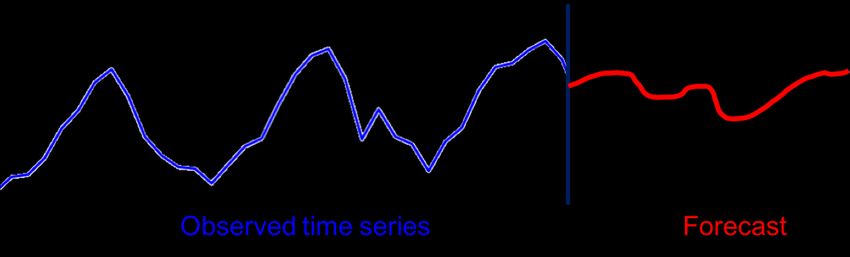
Figure 1 contains a summary of the forecasting problem when based on an observed
time series which exhibits a pattern (in this example, seasonality), a forecast is created
over a specified period. The horizontal axis represents time going from the past (left) to
the future (right). The vertical axis represents measured units. Given the past (in blue)
up to the vertical black line, identifying the future (in red) is the forecasting task.
2Amazon Web Services Time Series Forecasting Principles with Amazon Forecast
Figure 1 – Forecasting task overview
Considerations Before Attempting to Solve a
Forecasting Problem
The most important questions to understand before solving forecasting problems are: (i)
do you need to solve a forecasting problem? and (ii) why are you solving the forecasting
problem?
As a consequence of the ubiquity of time series data, it is easy to find forecasting
problems everywhere. However, a key question is whether there truly is a need for
solving a forecasting problem or whether you can circumvent it completely without
sacrificing efficient decision making in the business. Posing this question is important
because, scientifically speaking, forecasting is among the hardest problems in machine
learning.
For example, consider product recommendations for an online retailer. This product
recommendation problem can be framed as a forecasting problem where, for each
customer-stock keeping unit (SKU) pair, you forecast the number of units of a specific
item that this particular customer would purchase. This problem formulation has a
number of benefits, one benefit is that the time component is taken explicitly into
account, so you could recommend products according to the buying patterns of the
customers. However, product recommendation problems are rarely formulated as a
forecasting problem, since solving such a forecasting problem is much harder (e.g., the
sparsity of the information at the customer-SKU level and the scale of the problem) than
directly solving the recommendation problem. Therefore, as you think about a
forecasting application, it is important to consider the downstream usage of the forecast,
and whether it is possible to address this problem using an alternative approach.
Amazon Personalize can help in these cases. Amazon Personalize is a machine
learning service that makes it easy for developers to create individualized
recommendations for customers using their applications.
3Amazon Web Services Time Series Forecasting Principles with Amazon Forecast
After determining that you need to solve a forecasting problem, the next question to ask
is why are you solving the forecasting problem? In many business settings, forecasting
is usually just a means to an end. For example, for demand forecasting in a retail
context, the forecast may be used to make inventory management decisions. The
forecast problem is typically an input to a decision problem, which in turn may be
modeled as an optimization problem. Examples of such decision problems include the
number of units to be purchased or the best approach to deal with the existing
inventory. Other business forecasting problems include forecasting server capacity or
forecasting demand for raw materials/parts in a manufacturing context. These forecasts
may be used as inputs for other processes, either for decision problems as above, or for
scenario simulations, which are then used for planning without explicit models. There
are exceptions to the rule that forecasting is not an end in itself. In financial forecasting,
for example, the forecast is used directly to build up financial reserves or is presented to
investors.
To understand the purpose of the forecast, consider the following questions:
• How long into the future should you forecast for?
• How often do you need to generate forecasts?
• Are there specific aspects of the forecasts that you should dive deep into?
Case Study: Retail Demand Forecasting
Problem for an E-Commerce Business
To illustrate forecasting concepts in more detail, consider the case of an E-Commerce
business that sells products online. Optimizing decisions in the supply chain (e.g., in-
stock management) is critical to the core competitiveness of this business because it
helps having the accurate amount of products in the appropriate fulfillment locations.
This essentially means having a large selection available with shorter shipping times
and competitive prices which leads to higher customer satisfaction. The key input into
the supply chain software system is a prediction of demand or the forecast of potential
sales of every product in the catalog. This forecast enables important downstream
decisions, key among them being:
• Macro level planning (strategic forecasting): For a business as a whole,
what is the projected growth in terms of total sales/revenue? Where should the
business be (more) active geographically?
4Amazon Web Services Time Series Forecasting Principles with Amazon Forecast
• Purchase orders (operational forecasting): How many units of each product
should be purchased from the vendors and with what lead time, and also, in
what region should they be placed?
• Promotional activity (tactical forecasting): How should promotions be run?
Should products be liquidated?
The rest of the case study focuses on the second problem, which is part of the family of
operational forecasting problems (Januschowski & Kolassa, 2019). This document
follows the main concerns: data, models, improvements, and productization.
For this case study, it is important to keep in mind that the forecasting problem is a
means to an end. Although the forecasts are crucially important for the business, the
buying decisions are what is even more important. In our case study, these decisions
are taken by automated buying systems which rely on mathematical optimization
models from operations research. These systems try to minimize the expected cost for
the business. The key word here is expected, meaning that the forecasts ought to cover
not only one possible future but all possible futures, with the appropriate weighting
according to the probability of a particular outcome. To this end, the key enabler for
downstream decision making is a full distribution of the forecast values rather than just
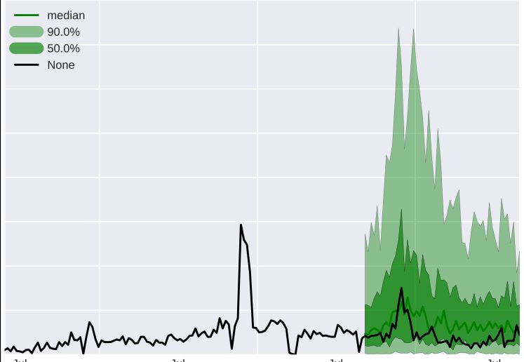
having a point forecast. Figure 2 shows a probabilistic forecast (also referred to as a
density forecast). Note that you can derive a single point forecast (e.g., the most likely
future) easily from this probabilistic forecast, but going from a point forecast to a
probabilistic forecast is more difficult.
Given a probabilistic forecast, you can obtain different statistics from it and tailor the
results to assist in the decision you want to take. The e-commerce business may have a
number of key products for which they almost never want to be out of stock. In this
case, use a high quantile (e.g., the 90-percentile) which would translate to 90% of the
time the products are going to be in-stock. For other products, such as products for
which replacements are more easily found (e.g., pencils), using a lower percentile may
be more appropriate.
In Amazon Forecast, you can obtain different quantiles from the probabilistic forecast
easily.
5Amazon Web Services Time Series Forecasting Principles with Amazon Forecast
Figure 2 – Illustration of probabilistic forecast: the black line is the actual values; the dark green
line is the median of the forecast distribution; the dark green shaded area is the prediction
interval into which you expect 50% of the values to fall; the light green area is the prediction
interval into which you expect 90% of the actual values would fall.
The following sections cover the steps involved for solving the forecasting problem for
this business, including data collection (Step 1), data preparation (Step 2), choosing a
model (Step 3), evaluating a forecast (Step 4), and automating forecast generation
(Step 5).
Step 1: Collect and Aggregate Data
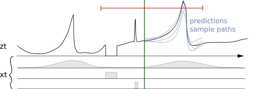
Figure 3 shows a mental model for the forecasting problem. The goal is to forecast the
time series z_t into the future (with uncertain estimation), using as much relevant
information as possible to make the forecast as accurate as possible. Therefore, the
first and most important step is to collect the right data and as much as possible of it.
6Amazon Web Services Time Series Forecasting Principles with Amazon Forecast
Figure 3 - A time series z_t together with associated features or co-variates (x_t) and multiple
forecasts (right from the green line) in blue which are samples of the probabilistic forecast
distribution (or, conversely, can be used to represent the probabilistic forecast).
The key information for a online retail business to record is:
• The transaction sales data: one possible schema is stock keeping unit (SKU),
timestamp, and units sold.
• SKU item details data: the metadata of an item. Examples include color,
department, size, etc.
• Price data: the price time series of each item with time stamps.
• Promotion information data: different types of promotions, either over a
collection of items (category) or individual items with time stamps.
• In-stock information data: for every unit of time, the information whether a
SKU was in-stock or purchasable.
Note that in-stock information is important since this problem centers on forecast
demand and not sales, but the business only records sales. When a SKU goes out of
stock, the number of sales is lower than the potential demand, so it is important to know
and record when such out-of-stock events occur.
Other datasets to consider include the number of webpage visits, details on search
terms, social media and weather information. It is often important to have data available
for the past and for the future to be able to use this data in models. The reasons for this
lies in it being a requirement of many forecasting models and in backtesting (described
in the Step 4: Evaluate Forecasts section).
For some forecasting problems, the frequency of the raw data naturally matches that of
the forecasting problem. Examples include the request of the server volume, which is
sampled by minute, and one wishes to forecast at minute frequency. Quite often, data is
7Amazon Web Services Time Series Forecasting Principles with Amazon Forecast
clocked at finer frequency or simply arbitrarily distributed across a time range, and the
forecasting problem is at a coarser granularity. This is a common occurrence in the
retail case study, where the sales data is normally recorded as event data, i.e., the
format consists of a timestamp with a fine granularity of when sales happened. In the
forecasting use case, this low granularity may not be needed and it may be more
appropriate to aggregate this data up into daily sales. Here, the level of aggregation
corresponds to the downstream problem, for example, inventory management.
Example
In Figure 4, the left graph shows an example of the raw customer sales data that can be
input to Amazon Forecast as a comma separated value (CSV) file. In this example, the
sales data is defined on a finer daily time grid, and the problem is to forecast the weekly
demand on the coarser time grid into the future. Amazon Forecast performs the
aggregation of the daily values in a given week in the create_predictor API call.
The result transforms the raw data into a collection of well-formed time series with a
fixed weekly frequency. The right graph illustrates this aggregation on the target time
series using the default summation aggregation method. Other aggregation methods
include averaging, maximum, minimum, or choosing a single point (e.g., the first) and
must be chosen such that it best matches the semantic of the data. In this example, the
aggregated value is aligned to the prior Monday of that week. Other aggregation
methods can be set by the user using the FeaturizationMethodParameters key
of the FeaturizationConfig parameter of the create_predictor API.
Figure 4 - Aggregation of raw sales data as events (left), into an equally-spaced time series
(right)
8Amazon Web Services Time Series Forecasting Principles with Amazon Forecast
Step 2. Prepare Data
Once you have raw data available, you need to handle complications, such as missing
data, and make sure that you prepare the data for the forecasting models such that the
data is amendable to them.
How to Handle Missing Data
A common occurrence in real-world forecasting problems is the presence of missing
values in the raw data. A missing value in a time series means that the true
corresponding value at every time point with the specified forecast frequency is not
available for further processing. There can be a multitude of reasons for values being
marked as missing. Missing values can occur because of no transaction, possible
measurement errors, e.g. a service that monitored certain data was not working
correctly, or because the measurement could not occur correctly. The primary example
for the latter in the retail case study is an out-of-stock situation in demand forecasting,
which means that demand does not equal the sales on that day. Similar effects can
occur in cloud computing scenarios when a service has reached a limit, e.g. Amazon
EC2 instances in a certain AWS Region are all busy. Another example of missing
values occurs when a product or service has not yet been launched or goes out of
production. Missing values can also be inserted by feature processing components, to
ensure equal lengths of the time series with padding.
Example
In Figure 5, the different strategies to handle missing values in Amazon Forecast, front,
middle and back filling, are illustrated for item 3 in a dataset of three items. The global
start date is defined as the earliest start date over the start dates of all the items. In the
below example, the global start date occurs for item 1. Similarly, the global end date is
defined as the latest end date of the time series over all items, which occurs for item 2.
Front fill fills in every value from the start of the particular time series to the global start
date. At the time of publishing this document, Amazon Forecast does not turn on any
front filling, and allows all the time series to start at different time points. Middle fill
denotes values that have been filled in the middle of the time series, and back fill fills
from the last date of that time series to the global end date.
9Amazon Web Services Time Series Forecasting Principles with Amazon Forecast
Figure 5 - Missing value handling strategies in Amazon Forecast. The global start date denotes
the earliest start date over the start dates of all the items, and the global end date denotes the
latest end date over the end dates of all items.
For middle and back fill, the default value in Amazon Forecast is zero filling. This is a
common scenario in the retail study that represents zero sales for transactional data for
available items. These values are treated as true zeros, and used in the metrics
evaluation component. Amazon Forecast also allows the user to identify values that are
actually missing and encode them as NaNs (not a number) for the algorithms to
process. Let’s examine why these two cases differ and when each is useful.
In the retail case study, the information that a retailer sold zero units of an available item
differs from the information that zero units of an unavailable item are sold either in the
periods outside its existence, e.g. before its launch or after its deprecation, or in periods
within its existence, e.g. partially out of stock, or when there was no sales data recorded
for this time range. The default zero filling is applicable in this former case. In the latter,
even though the corresponding target value is typically zero, there is additional
information conveyed in the value being marked as missing. You must preserve the
information that there was missing data and not discard this information (see the
following example for an illustration why keeping the information is important). To
encode a value that does not represent zero sales of an available product as truly
missing, Amazon Forecast allows the user to specify the filling type for middle fill and
back fill in the FeaturizationMethodParameters key of the
FeaturizationConfig parameter of the create_predictor API. To mark a
value as truly missing, the fill type for these parameters should be set to NaN. Unlike for
zero filling, the values encoded with NaN are treated as truly missing, and not used in
the metrics evaluation component.
10Amazon Web Services Time Series Forecasting Principles with Amazon Forecast
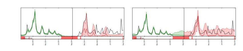
Figure 6- The effect of 0-filling vs filling by NaN on the forecasts for the same item. In the left
graph, the values left to the vertical black line are filled with 0s, leading to an under-biased
forecast (to the right of the vertical black line). In the right graph, these values are marked as
NaN, leading to appropriate forecasts
Example
Figure 6 illustrates the importance of handling missing values correctly for a linear state
space model, such as ARIMA or ETS. It plots the demand forecast for an item that is
partially out of stock. The training region is shown in the left graph in green, the
prediction range in the right panel in red and the true target in black. The median, p10
and p90 forecasts are shown in the red line and the shaded region, respectively. The
bottom shows the out of stock items (80% of the data) marked in red. In the left plot, the
out of stock regions are ignored and filled by 0. This results in the forecast models
assuming that there are a lot of zeros to predict and therefore the forecasts are too low.
In the right plot, the out of stock regions are treated as true missing observations and
the demand becomes uncertain in the out of stock region. With the missing values for
the out of stock items appropriately marked as NaN, you see no under-bias in the
prediction range in this plot. Amazon Forecast fills in these gaps in data making it easy
for the user to correctly handle missing data, without requiring the user to explicitly
modify all of their input data.
Concepts of Featurization and Related Time Series
Amazon Forecast allows users the ability to input related data to help improve the
accuracy of certain supported forecasting models. This data is broken into two cases:
related data that are time series and static data, typically metadata.
Note: Metadata is referred to as features in machine learning, and co-
variates in statistics.
Related time series are time series that have some correlation with the target value, and
should lend some statistical strength to forecast on the target value because they
11Amazon Web Services Time Series Forecasting Principles with Amazon Forecast
provide an explanation in intuitive terms (see Amazon Forecast: predicting time-series
at scale for an example). Unlike the target time series, related time series are known
values in the past that may impact the target time series, and they must have known
values in the future. Common examples in the retail case study include price,
promotions, whether a day is a weekday or weekend, and holidays.
Example
Figure 7 shows an example of how related time series can be used to predict the future
demand of a popular book. The blue line represents the demand in the target time
series. The price is shown as the green line. The vertical red line represents the
forecast start date, and two quantile forecasts are shown to the right of the red line. The
related time series aligns with the target time series at the forecasting granularity, and is
known at all times in the future in the range of the forecast start date to the forecast start
date incremented by the forecast horizon (forecast end date).
Related time series must be known for the entirety of the forecast horizon in Amazon
Forecast and must be specified at the same frequency as the forecast frequency. At the
time of writing, this is a technical prerequisite for all current models in Amazon Forecast.
In many practical scenarios, this prerequisite is not overly restrictive. Continuing the
example of prices, in the absence of future prices, you can use a simple workaround.
Instead of dealing with absolute price, it may be better to use price changes (either the
absolute difference or the relative difference to a base price) and assume the price to be
of a certain value in the future (e.g., the base price).
Figure 7 also shows that the price is a suitable feature to use, since you can see
correlations between a decrease in price with an increase in sales of the product.
Related time series can be supplied to Amazon Forecast through a separate CSV file,
containing the item SKU, timestamp and related time series values (i.e. price in this
case). Since related time series are defined to be known at every time point, unlike
target time series, missing values are not supported at the time of writing this document,
and every value must be provided in the CSV. The natural notion of aggregation, e.g.
summation, as discussed for target time series does not exist and is not supported for
related time series at the time of writing. For example, it makes little sense to sum a
daily price to a weekly price, and similarly for daily promotions. Amazon Forecast can
automatically include holidays for different countries as a related time series (see
SupplementaryFeature for the current list of supported country values). Holidays can be
especially useful to help predict retail spikes around holidays, such as Thanksgiving and
Christmas.
12Amazon Web Services Time Series Forecasting Principles with Amazon Forecast
Figure 7 - The sales of a particular item (in blue, left to the vertical red line)
Item metadata, also known as categorical variables, are other helpful features that can
be input to Amazon Forecast (see Amazon Forecast: predicting time-series at scale for
an example). The main difference between categorical variables and related time series
is that categorical variables are static, that is, they do not change over time. Common
retail examples include the colors of items, categories of books, and binary indicators of
whether a TV is a smart TV or not. This information can be picked up by deep learning
algorithms in learning similarities between SKUs assuming that similar SKUs have
similar sales. Since this metadata does not have a time dependency, each row in the
item metadata CSV file only consists of the item SKU and the corresponding category
label or description.
Step 3: Choose a Model
Most classical forecasting methods fit a single model to each individual time series, and
then use that model to extrapolate the particular time series into the future. These
models are referred to as local models because there is a local model per SKU.
Amazon Forecast provides scalable versions of the popular local models from the R
forecast package, ARIMA and ETS. Amazon Forecast also includes the Python
implementation of Bayesian structural time series model Prophet. We provide black-box
implementations of these common open-source algorithms for simple comparison and
benchmarking of the various methods, either by invoking them individually or
automatically with the AutoML feature (Amazon Forecast automatically chooses an
algorithm for you by performing model selection). NPTS (non-parametric time series) is
a local method developed at Amazon, which is similar to the simple forecasters but with
a key difference. Unlike the simple or seasonal simple forecasters (which just repeat the
last value or the value at the appropriate seasonality and hence provide point
forecasts), NPTS produces probabilistic forecasts. NPTS use a fixed-time index, that is,
the previous index T - 1 or the past season T - tau as the prediction for time step T,
13Amazon Web Services Time Series Forecasting Principles with Amazon Forecast
respectively, NPTS randomly samples a time index t in the set {0, ..., T - 1} in the past
to generate a sample for the current time step T. NPTS is another good baseline model
to benchmark the deep learning methods against. In particular for intermittent
(sometimes also called sparse) time series, that is, time series with many zeros, NPTS
can be a highly effective method.
The global deep learning algorithm, DeepAR+, trains a single model jointly over the
entire collection of the time series in the dataset. This can be beneficial in applications,
where there are similar time series across a set of cross-sectional units. Examples of
these time series groupings include demand for different products, server loads, and
requests for web pages. For these problems, DeepAR+ can outperform the standard
methods, such as ARIMA and ETS. In general, as the number of time series increases,
the efficacy of DeepAR+ increases but the same is not true for local models. The trained
model can also be used for generating forecasts for new SKUs without historical sales
(also called the cold start problem, see Forecast with Cold Start Items for an example).
Amazon Forecast allows you to choose a specific local or deep learning algorithm, or
choose AutoML, a functionality by which Amazon Forecast automatically chooses an
algorithm for you by performing model selection. Figure 8 shows a pyramid illustration of
these algorithms provided in Amazon Forecast. AWS continues to add and enhance
forecasting algorithms used in Amazon Forecast.
Figure 8 - Hierarchy of models available in Amazon Forecast
Step 4: Evaluate Forecasts
A typical workflow in machine learning consists of training a set of models or
combination of model(s) on a training set and assessing its accuracy on hold out data
sets, e.g., test and validation data sets. This section discusses how to split historic data,
and which metrics to use to evaluate models in time series forecasting. For forecasting,
14Amazon Web Services Time Series Forecasting Principles with Amazon Forecast
this backtesting is the main tool to assess forecast accuracy and given the
consequences of forecasting, accuracy really matters.
Backtesting
A proper evaluation and backtesting framework is among the most important factors in
turning a machine learning application into a success. You can rely on successful
backtests with your models to gain confidence over the models’ future predictive power.
Furthermore, you can tune models via hyper-parameter optimization (HPO), learn
model combinations, and enable meta-learning and AutoML.
The time series forecasting characteristic time makes it different, in terms of evaluation
and backtesting methodology, from other fields of applied machine learning. Usually in
ML tasks, to assess the predictive error in a backtest, you split a data set by items. For
example, for cross-validation in image-related tasks, you train on some percentage of
the pictures, and then use other parts for testing and validation. In forecasting, you need
to split primarily by time (and to a lesser degree by items) to ensure that you do not leak
information from the training set into the test or validation set, and that you simulate the
production case as closely as possible.
The split by time must be done carefully because you do not want to choose a single
point in time, but multiple points. Otherwise, the accuracy is too dependent on the
forecast start date, as defined by the splitting point. A rolling forecast evaluation, where
you do a series of splits over multiple time points, and output the average result leads to
more robust and reliable backtest results. Figure 9 illustrates four different backtest
splits.
15Amazon Web Services Time Series Forecasting Principles with Amazon Forecast
Figure 9 - Illustration of four different backtesting scenarios with increasing training set size, but
constant size of testing. All backtesting scenarios have data available during its entirety to be
able to evaluate forecasted values against actuals.
The reason that multiple backtest windows are needed is that most time series in the
real world are normally non-stationary. The e-commerce business in the case study is
based in North America and much of its product demand is driven by the Q4 peak, with
particular peaks around Thanksgiving and before Christmas. In the Q4 shopping
season, the variability of the time series is higher than the rest of the year. By having
multiple backtest windows, you can evaluate forecasting models in a more balanced
setting.
For each backtest scenario, Figure 10 shows the basic elements in the terminology of
Amazon Forecast. Amazon Forecast automatically splits the data into the train and test
datasets. Amazon Forecast decides how to split the input data by using the
BackTestWindowOffset parameter that is either specified as a parameter in the
create_predictor API or uses its default value of ForecastHorizon. In the
following figure, you see the more general former case when the
BackTestWindowOffset and ForecastHorizon parameters are not equal. The
BackTestWindowOffset parameter defines a virtual forecast start date, shown as
the dashed vertical line in Figure 10. It can be used to answer the following hypothetical
question: if the model is deployed on this day, what would the forecast be? The
ForecastHorizon defines the number of time steps from the virtual forecast start
date to predict.
16Amazon Web Services Time Series Forecasting Principles with Amazon Forecast
Figure 10 - Illustration of a single backtest scenario and its configuration in Amazon Forecast.
Quantile Losses and Probabilistic Forecasts
This section discusses which accuracy metrics are useful in evaluating the forecasts
and why the quantile losses are preferred for these probabilistic forecasts. The
discussion is mathematical and not necessary for understanding the rest of this paper.
Amazon Forecast outputs probabilistic forecasts, which contain a prediction interval.
This contrasts with point forecasts, which consist only of the forecasted values. The
result gives prediction quantiles, known as intervals, which can be used to express the
uncertainty in the forecasts. By calculating prediction quantiles, the model shows how
much uncertainty is associated with each forecast, and therefore provides further
information to the user. Without prediction quantiles, point forecasts have limited value
for downstream decision making.
Generating forecasts at different quantiles is particularly useful when the costs of under
and over predicting are different. Amazon Forecast can generate probabilistic forecasts
at any quantile. In the case study, forecasts are generated at three quantiles—p10, p50,
and p90. The weighted quantile loss (wQuantileLoss) calculates how far the forecast is
from actual demand in either direction as a percentage of demand on average in each
quantile. This metric helps capture the inherent bias in each quantile. The lower
wQuantileLoss errors indicate better overall accuracy of the forecast. The weighted
quantile loss is given as:
17Amazon Web Services Time Series Forecasting Principles with Amazon Forecast
where q(tau) is the tau - quantile that the model predicts for tau in the set {0.1, 0.2, ,...,
0.9}, and y is the exact target value at the corresponding item index i, ranging from 1 to
the total number of items n and time index t, ranging from 1 to the final time T in the
evaluation period. Amazon Forecast calculates the weighted p10, p50, and p90 quantile
losses, where tau is in the set {0.1, 0.5, 0.9}, respectively, which covers the standard
80% prediction interval region.
For the p10 forecast, the true value is expected to be lower than the predicted value
10% of the time, and the wQuantileLoss[0.1] can be used to assess its accuracy. For a
use case when there is not a lot of storage space and the cost of invested capital is
high, or the price of being overstocked on an item is of concern, the p10 quantile
forecast is useful to order a relatively low number of stock. The p10 forecast over-
estimates the demand for an item only 10% of the time, meaning that approximately
90% of the time, that item will be sold out.
For the p50 forecast (often also called the median) the true value is expected to be
lower than the predicted value 50% of the time, and the wQuantileLoss[0.5] can be used
to assess its accuracy. When being overstocked is not too concerning, and there is a
moderate amount of demand for a given item, the p50 quantile forecast can be useful.
For the p90 forecast, the true value is expected to be lower than the predicted value
90% of the time, and the wQuantileLoss[0.9] can be used to assess its accuracy. When
being understocked on an item will result in a large amount of lost revenue, that is, the
cost of not selling the item is extremely high or the cost of invested capital is low, the
p90 forecast can be useful to order a relatively high number of stock.
Example
This example combines all these quantile forecasts for the retail case study. In this
example, you want to forecast the product demand for gloves that sell well during the
fall and winter seasons. Quantiles forecasts are a tool that can help determine how
many gloves to order. If the main concern is not running out of stock, a high quantile
forecast, like the p90 or p99 quantile forecast, would be recommended. However, even
though the demand forecast would be lower for the spring season, a high percentile
may—— still lead to overstock in the spring. On the other hand, if the main concern is
not being over-stocked in the spring, the p10 quantile forecast would be recommended.
This has the associated risk of selling out during the winter. The p50 quantile forecast
gives a balance between the two.
18Amazon Web Services Time Series Forecasting Principles with Amazon Forecast
Problems with MAPE and RMSE
In most cases, the point forecasts that can be generated internally or from other
forecasting tools should match the p50 quantile forecasts. For tau = 0.5 in the
wQuantileLoss[tau] equation, both weights are equal, and the wQuantileLoss[0.5]
reduces to the commonly used Mean Absolute Percentage Error (MAPE) for point
forecasts:
where yhat = q(0.5) is the compute forecast. A scaling factor of 2 is used in the
wQuantileLoss formula to cancel the 0.5 factor to obtain the exact MAPE expression.
Note that the above definition of MAPE differs from a common interpretation for MAPE.
The difference is in the denominator. The way MAPE is defined above avoids the
problem of division by 0, a commonly occurring problem in real-world scenarios such as
the e-commerce business in the case study, which will often sell 0 units of a given SKU
on a given day.
Unlike with the weighted quantile loss metric for tau not equal to 0.5, the inherent bias in
each quantile cannot be captured by a calculation like the MAPE, where the weights are
equal. Other disadvantages of the MAPE include that it is not symmetric, has an over
inflation of percentage errors for small numbers, and is just a point-wise metric.
The RMSE is the square of the error term in the MAPE and a common error metric in
other ML applications. The RMSE metric favors a model, where the individual errors are
of consistent magnitude, as large variations in error will increase the RMSE over-
proportionally. Due to the squared error, a few poorly predicted values in an otherwise
good forecast can increase the RMSE. Also, because of the squared terms, smaller
error terms have less weight in the RMSE than in the MAPE. For the RMSE, Amazon
Forecast uses the p50 forecast to represent the predicted value, i.e. yhat = q(0.5).
19Amazon Web Services Time Series Forecasting Principles with Amazon Forecast
The above metrics allow for a quantitative assessment of the forecasts. In particular for
large scale comparisons (is method A better than method B overall), these are crucial.
However, complementing this with visuals for individual SKUs is often important.
Step 5: Generate Forecasts and Use Forecasts
for Decision Making
Once you have a model that meets the accuracy threshold required for your specific
use case (as determined via backtesting), the final step involves deploying the model
and generating forecasts. To deploy a model in Amazon Forecast, you must run the
Create_Forecast API. This action hosts a model created by training on the entire
historical dataset (unlike Create_Predictor which splits the data into a train and
test set). The model predictions generated over the forecast horizon can be then be
consumed in two ways:
• You can query the forecasts for a particular item or combination of
item/dimension using the Query_Forecast API from the AWS CLI or directly
via the AWS Management Console.
• You can generate the forecasts for all combination of items and dimensions
across all quantiles using the Create_Forecast_Export_Job API. This
API generates a CSV file that is securely stored in an Amazon S3 location of
your choice. You can then use data from the CSV file and plug them into your
downstream systems used for decision making. For example, your existing
supply chain systems can ingest the output from Amazon Forecast directly to
help inform decision making around manufacturing of specific SKUs.
Visualization
Amazon Forecast allows for the plotting of forecasts natively in the AWS Management
Console (Figure 11). Additionally, you can take advantage of the complete Python data
science stack (see Evaluating Your Forecast). Amazon Forecast allows for the
exporting of forecasts as a CSV file via the ExportForecastJob API, which allows
users to visualize the forecast in their analytic tool of choice.
20Amazon Web Services Time Series Forecasting Principles with Amazon Forecast
Figure 11: Visualization provided in the Amazon Forecast console at different quantiles
Summary of Forecasting Workflow and APIs
The following table matches each step of the forecasting workflow with the respective
Amazon Forecast API.
Table 1: Forecasting steps and Amazon Forecast APIs
Step API API Functions
Step 1: Collect and Create_Dataset_Group, 1. Establish the high level
Aggregate Data Create_Dataset, domain (e.g. Retail,
Create_Dataset_Import_Job Metrics etc.) for the
Step 2. Prepare Data problem.
2. Define the schema for the
different datasets (target,
related, item-metadata.
3. Import data from Amazon
S3 into Amazon Forecast.
Step 3: Choose a Create_Predictor 1. Performs the ETL.
Model 2. Splits data into train/test
sets and trains the model.
Step 4: Evaluate
Forecasts 3. Generates metrics to
evaluate model accuracy.
21Amazon Web Services Time Series Forecasting Principles with Amazon Forecast
Step API API Functions
Step 5: Generate Create_Forecast 1. Trains/hosts the model.
Forecasts and Use 2. Generates predictions over
Forecasts for the forecast horizon for a
Decision Making specific quantile of interest
(i.e. any integer between 1
to 99 including mean).
Query_Forecast Allows you to consume the
Create_Forecast_Export_Job forecasts created by
Create_Forecast
Using Amazon Forecast for Common Scenarios
You can also conduct what-if analysis by generating different forecasts based on
changes in external variables (e.g. price, weather etc.). For example, in the e-commerce
case study example, you can create different forecasts based on promotions that you
may be planning. You can forecast demand for a product at 10% discount and then at
20% discount to understand the quantity of product that you would need to stock to
meet demand. This can be achieved by setting up unique dataset groups and updating
the related time series in each, based on the scenario of interest. Additionally, you can
also generate forecasts for items with no prior history. This approach requires creating a
predictor using DeepAR+ along with metadata (i.e. item metadata dataset) to generate
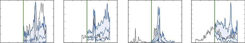
forecasts for the new item. Figure 12 shows examples of 4 different SKUs as they
appear in real-world operational forecasting problems.
Figure 12 - Examples of 4 different SKUs as they appear in real-world operational forecasting
problems. Left to the green line are the observed actuals, right to the green line is a forecast (in
blue) compared with the actuals in black. Note that each individual’s SKU’s history, left to the
green line, is not indicative of the evolution of it right to the green line.
22Amazon Web Services Time Series Forecasting Principles with Amazon Forecast
Implementing Forecast into Production
Having completed the end-to-end Amazon Forecast workflow, it is critical to identify key
differences between the Create_Predictor and Create_Forecast APIs and
when each should be used. The former is used primarily during proof of concept in
order to evaluate model accuracy/metrics, whereas the latter is used to generate
forecasts in a production environment. Once in production, Create_Predictor does
not need to be run every time a forecast needs to be generated but only when the
model needs to be retrained due to changes in data or as part of a pre-established
cadence (i.e. bi-weekly or monthly). Essentially as the datasets are updated with new
data, only Create_Forecast needs to be run to generate forecasts for the new
forecast horizon.
In production, you also need to automate your dataset imports and forecast operations
in order to generate new predictions on a rolling basis. Today, this can be achieved by
setting up cron jobs using a combination of Amazon CloudWatch Events logs, AWS
Step Functions, and AWS Lambda functions. The cron job setup in turn automates
Amazon Forecast API calls for import/re-train or forecast generation. Finally, it is also
key to manage your resources and delete them at regular intervals so that you do not
exceed system limits prescribed by the service.
Conclusion
Januschowski and Kolassa (2019) provide a classification of forecasting problems
aligned with the decisions businesses need to take, including strategic, tactical, and
operational decisions. Each decision level has corresponding forecasting tasks.
Operational and tactical forecasting problems are characterized as containing large
amounts of data, and typically require a high degree of automation. Different forecasting
methods cater for these problems. Local forecasting methods typically work well for
strategic forecasting problems, deep learning based methods for operational forecasting
problems and for the in-between, a bit of experimentation may be necessary. Although
this paper discussed operational forecasting problems, Amazon Forecast is not
opinionated about the models it offers and includes models that serve strategical as well
as operational and tactical forecasting problems.
The operational forecasting problem solving process can be broken into basic steps
starting from data collection and preparation to model building and deployment. In
general, it is most useful to regard this is an iterative, rather than a linear process. For
example, as models and use cases are better understood, it may make sense to go
23Amazon Web Services Time Series Forecasting Principles with Amazon Forecast
back to the data collection phase. Model development is also highly iterative in itself
(Figure 13).
Figure 13 - A simplified development process of bringing a forecasting model to production.
Contributors
Contributors to this document include:
• Yuyang Wang, Senior Machine Learning Scientist, AI Vertical Services
• Danielle Robinson, Applied Scientist, AI Vertical Services
• Tim Januschowski, Manager, ML Applied Science
• Rohit Menon, Senior Product Manager, AI Vertical Services
• Namita Das, Senior Product Manager, AI Vertical Services
Further Reading
For additional information on time series forecasting and deep learning methods, see:
• Amazon Forecast Documentation
• Amazon Forecast general availability blog
• Now available in Amazon SageMaker: DeepAR algorithm for more accurate
time series forecasting
24Amazon Web Services Time Series Forecasting Principles with Amazon Forecast
• Amazon SageMaker DeepAR now supports missing values, categorical and
time series features, and generalized frequencies
• Scientific papers on time series forecasting models
Document Revisions
Date Description
February 2020 First publication.
25Amazon Web Services Time Series Forecasting Principles with Amazon Forecast
Appendix A: FAQs
Q: How many data points per item combination do we need at a minimum?
This is impossible to quantify rigorously and we can only rely on rules of thumb. The
general rule is, as with most Machine Learning problems: the more the better. This
holds true in particular for deep learning based models. To answer this question more
effectively, trial-and-error is the most effective path forward.
Q: How to think about missing data? When is it too much to generate reasonable
forecasts?
If a large portion of the data is missing, this typically points to a problem in the data
collection phase. It may be the case that there are problems in the recording of data or
that the aggregation level of the data is too low.
Q: How can I improve the Forecasting Accuracy?
The most important question to answer is first, whether we indeed have a forecasting
problem and second, if we have the right data available in the right amount of quantity
and quality. If accuracy is dissatisfactory, it may make sense to understand how
predictable the problem is (or, put differently, how random/noisy/stationary is the data)
Q: For Deep Learning Models such as DeepAR, how much data is enough?
What’s the general guidance of tuning DeepAR?
The rule of thumb is 10k data points (where each point is a single point in a time series;
e.g., 1 year of daily data for 30 products) are roughly necessary, but this depends on
the predictability of the data.
Q: I have a model that works very well for my use case, and it is not offered in
Amazon Forecast, what should I do?
The Amazon Forecast team will be glad to help you with this use case. Please contact
the service team of Amazon Forecast by emailing amazonforecast-poc@amazon.com.
26Amazon Web Services Time Series Forecasting Principles with Amazon Forecast
Appendix B: References
Januschowski, Tim and Kolassa, Stephan. A classification of business forecasting
problems. Foresight: The International Journal of Applied Forecasting. 2019
Salinas, David, Flunkert, Valentin, Gasthaus, Jan and Januschowski, Tim. DeepAR:
Probabilistic forecasting with autoregressive recurrent networks. International
Journal of Forecasting. 2019
Gasthaus, Jan, Benidis, Konstantinos, Wang, Yuyang, Rangapuram, Syama Sundar,
Salinas, David, Flunkert, Valentin and Januschowski, Tim. {Probabilistic
Forecasting with Spline Quantile Function RNNs. The 22nd International
Conference on Artificial Intelligence and Statistics. 2019.
Januschowski, Tim, Gasthaus, Jan, Wang, Yuyang, Salinas, David, Flunkert, Valentin,
Bohlke-Schneider, Michael and Callot, Laurent. Criteria for classifying forecasting
methods. International Journal of Forecasting. 2019.
Januschowski, Tim, Gasthaus, Jan, Wang, Yuyang, Rangapuram, Syama and Callot,
Laurent. Deep Learning for Forecasting. Foresight: The International Journal of
Applied Forecasting. 2018
Januschowski, Tim, Gasthaus, Jan, Wang, Yuyang, Rangapuram, Syama Sundar and
Callot, Laurent. Deep Learning for Forecasting: Current Trends and Challenges.
Foresight: The International Journal of Applied Forecasting. 2018.
Bose, Joos-Hendrik, Flunkert, Valentin, Gasthaus, Jan, Januschowski, Tim, Lange,
Dustin, Salinas, David, Schelter, Sebastian, Seeger, Matthias and Wang,
Yuyang. Probabilistic demand forecasting at scale. Proceedings of the VLDB
Endowment. 2017
27You can also read