Weekly Disambiguations of US Patent Grants and Applications

Page created by Rafael Nelson

Education

English

Like
Share
Embed
Fullscreen
Slides
Download HTML
Download PDF
Abuse

←

→

Page content transcription

If your browser does not render page correctly, please read the page content below

Weekly Disambiguations of US Patent Grants and Applications

Weekly Disambiguations of US Patent Grants and Applications

                                          Gabe Fierro
                                       Benjamin Balsmeier
                                         Guan-Cheng Li
                                         Kevin Johnson
                                         Aditya Kaulagi
                                            Bill Yeh
                                          Lee Fleming

                                         January 3, 2014

Benjamin Balsmeier KU Leuven, Department of Managerial Economics, Strategy and
Innovation, Benjamin.Balsmeier@kuleuven.be

Gabe Fierro
UC Berkeley, Coleman Fung Institute for Engineering Leadership, gtfierro@berkeley.edu

Lee Fleming
UC Berkeley, Coleman Fung Institute for Engineering Leadership, lfleming@ieor.berkeley.edu

Kevin Johnson
UC Berkeley, Electrical Engineering and Computer Science, vadskye@gmail.com

Aditya Kaulagi
UC Berkeley, Electrical Engineering and Computer Science, aditya15@berkeley.edu

Guan-Cheng Li
UC Berkeley, Coleman Fung Institute for Engineering Leadership,
guanchengli@eecs.berkeley.edu

William Yeh
UC Berkeley, Electrical Engineering and Computer Science, billyeh@berkeley.edu

                                             1

Abstract
We introduce a new database and tools that will ingest and build an updated database each
week using United States patent data. The tools disambiguate inventor, assignee, law firm,
and location names mentioned on each granted US patent since 1975 and all applications
since 2001. While parts of this first version are crude, all the approaches are fully automated
and provide the foundation for much greater improvement. We describe a simple user
interface, provide some descriptive statistics, and discuss matching the disambiguated patent
data with other frequently used datasets such as Compustat. The data and documentation can
be found at http://www.funginstitute.berkeley.edu/.

JEL-Classification:
Keywords:                  Disambiguation, Patent Data, Economics of Science, Innovation
                           Policy Research

* The Authors gratefully acknowledge the Coleman Fung Institute for Engineering Leadership,
the National Science Foundation (grant # 1064182), the United States Patent and Trademark
Office, and the American Institutes for Research. Jeff Oldham and Google provided crucial help
in the location disambiguation. Balsmeier gratefully acknowledges financial support from the
Flemish Science Foundation. This paper pulls directly from technical notes by the same authors,
available from the Fung Institute website: http://www.funginstitute.berkeley.edu/publications.

                                                 2

Introduction

Patent data has been used to study invention and innovation for over half a century (see

e.g. Schmookler, 1966; Scherer, 1982; and Griliches, 1984, for early influential studies and Hall

et al., 2012 for a recent overview). The popularity of patent data stems largely from the rich,

consistent, and comparable information that can be obtained for a huge amount of entities, i.e.

organizations, individuals, and locations. Aggregating patents is, however, not straightforward

because entities (inventors, assignees, applicant law firm, and location) are only listed by their

names on each patent document and receive no unique identifier from the patent office

(essentially inconsistent text fields). Looking at these fields as they appear on the patent

document reveals various forms of misspellings or correct but different name spellings that

hinder an easy aggregation. The ambiguous names further limit the possibility to assemble patent

portfolios for research as it is difficult to foresee all the kinds of name abbreviations that can

occur. As a result, individual researchers have often spent significant amounts of time and

resources on labor-intensive manual disambiguations of relatively small numbers of patents. The

intent of this paper is to provide a working prototype for automating the disambiguation of these

entities, with the ultimate goal of providing reasonably accurate and timely (ideally, every week)

disambiguation data.

A wide variety of efforts have recently been made to disambiguate inventor names

(Fleming and Juda 2004; Singh 2005; Trajtenberg et al., 2006; Raffo and Lhuillery 2009;

Carayol and Cassi, 2009; Lai et al., 2009; Pezzoni et al., 2012, Li forthcoming). These efforts

are gaining in sophistication, accuracy, and speed, such that fully automated approaches can now

compete with smaller and hand crafted and manually tuned datasets.

Concurrent efforts have been made at the assignee level using automated and manual

methods. Hall et al. (2001) disambiguated the assignees and introduced their patent data project

under the umbrella of the National Bureau of Economic Research (NBER). These data are

widely used, partly because many assignees have also been matched to unique identifiers of

publicly listed firms, which in turn enables easy matching with various other firm level

databases, e.g. Compustat. Producing updates of the NBER patent data is costly, however, due to

the quite sophisticated but still labor-intensive assignee disambiguation process.

Many patent applications contain information about the applicant’s law firm (though an

inventor or his/her employer need not retain a law firm, many do); however, to the best of our

knowledge, this field has never been disambiguated. Identifying unique law firms could aid in

understanding patent pendency and disambiguation of other fields. Location data are available

for most inventors (their home towns in particular) and while these data have been exploited,

there does not exist a comprehensive and automated approach to disambiguating these data.

To further aid the research community, this paper also includes application data for all

these fields as well. Almost all research to date has used granted patent data, which ignores the

many applications that were denied, and might introduce bias. Application data have been

recently made available by the USPTO, but to our knowledge, not been made easily available to

the research community yet.

Here we introduce four automated disambiguation algorithms: inventor, assignee, law firm,

and location. The latter three need much further accuracy improvement but they are fast enough

to disambiguate over 6 million patents and pending applications within days, and thus enable

weekly updates on all USPTO granted patents and applications. Application data since 2001 are

included as well. A simple user interface that emails data to users is available and documented

below. Code is available from the last author to any non-profit research organization. For

updates and addresses to authors, data, tools and code, please see

http://www.funginstitute.berkeley.edu/.

Data	
  sources	
  

       We developed a fully automated tool chain for processing and providing patent data

intended for research, illustrated in Figure 1 (for technical details see Fierro, 2013). As data is

downloaded from the USPTO weekly patent releases hosted by Google, it is parsed, cleaned and

inserted into a SQL database. The output data from these processes are combined with data from

the Harvard Dataverse Network (DVN, see Li et al. forthcoming), which itself consists of data

drawn from the National Bureau of Economic Research (NBER), weekly distributions of patent

data from the USPTO, and to a small extent, the 1998 Micropatent CD product. Disambiguations

begin from this database.

                                                  5

Figure 1: Tool and data flow for weekly disambiguations of US patent grant and application data.

      Every week, the USPTO releases a file of documents the patents granted the prior week.

Since the inception of digital patent record release in 1976, the USPTO has used no less than 8

different formats for representing granted patents alone. Patents granted since 2005 are available

in various XML (Extensible Markup Language) schemas, which allows the development of a

generalized parser to extract the relevant information from the patent documents. The Fung

Institute parser transforms XML documents from the canonical tree-based structures into lookup

tables. Typical XML parsers must be tailored to the exact structure of their target documents, and

must maintain a careful awareness of contingent errors in the XML structure. The Fung Institute

parser circumvents this issue by using generalized descriptors of the desired data instead of

explicit designation. This robust approach allows the parser to handle small schema changes

without adjustment, decreasing the need for constant development.

                                                 6

As the data is extracted from USPTO documents, it is streamed into a relational database

that contains records linking patents, citations, inventors, law firms, assignees, technology

classes and locations. The database itself is MySQL, but the patent library uses an object

relational mapper (ORM) to allow database entries to be manipulated as Python objects. This

simplifies development by removing the need to write code for a specific database backend, and

facilitates use by not requiring the user to be familiar enough with relational databases in order to

query and manipulate data. The database is structured such that the data, as it is extracted from

the source files, is inserted into “raw” tables that preserve the original resolution of the data. The

unaltered records present problems when attempting to group data by common features. As the

disambiguations are run, the raw records are linked to the disambiguated records.

      Figure 2: Abstract view of relational database for patent grant and application data.

                                                  7

Algorithms	
  

Inventors	
  1	
  

           We treat inventor disambiguation as a clustering problem; to disambiguate names, we seek

high intra-cluster similarity and low inter-cluster similarity amongst patent-inventor pairs. While

conceptually simple, the challenge is to accurately and quickly cluster approximately 6 million

patents and applications and over 10 million names.

           Step 1: Vectorization

           We define a document unit of a patent as an unordered collection of that patent’s attributes.

The current version attributes are 1) inventor name 2) co-authors (implicitly, by association on

the same patent), 3) assignees, 4) patent class, and 5) location. The occurrence of each attribute

is used as a feature for training a classifier. We build a document-by-attribute incidence matrix,

which is sparse because a patent cannot use all possible attributes. Figure 3 illustrates.

           Figure 3: Document by attribute matrix.

       1
   The following is taken directly from an internal technical report by Guan-Cheng Li:
http://www.funginstitute.berkeley.edu/sites/default/files/Disambiguation%20of%20Inventors%2C%20USPTO%201
975%20%E2%80%93%202013.pdf.

                                                      8

Suppose one or more inventors named John Davis have filed five patents, A, B, C, D, E. Let

the inventors named John Davis initially be one column (depicted by the black vertical tab in

Figure 3). We look closer at the five rows that have ‘1’s along that column, namely the index of

the patents being filed by John Davis. Having formed a matrix, we can compute correlations

between rows (patents) and columns (inventors).

Step 2: Distance measurements

Distance measurements can be computed in a number of ways, e.g., Euclidean distance,

Manhattan distance or Chebyshev distance. They enable quantization of the dissimilarity that an

inventor varies from the rest of the other inventors. Here, we adopt the Euclidean distance.

(1)

Step 3: Splitting the same inventor name by inter-clustering

Common names usually represent multiple persons, e.g., John Davis. If, for example, there

were four such different people across the USPTO dataset, the algorithm should cluster and

report four unique identifiers for John Davis.

We examine the inventor block and extract a list of unique inventor names. To initialize, we

treat each individual inventor as a distinct person, e.g., by assigning initial identifiers. Then, we

cluster each inventor block that is centered by the inventor names, i.e., John Davis as an

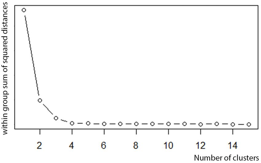
example, by applying the k-means clustering algorithm based on a bottom-up approach. When

splitting, we calculate the new means to be the centroids of the observations in the new clusters.

Figure 4: The optimal number of clusters is determined by the point of decreasing returns (5
in this example).

     We determine the cluster size by minimizing the sum of each clusters’ sum of the inter-

cluster’s squared distances. As illustrated in Figure 4, the five names, John Davis, are grouped

down to four clusters. When the sum no longer decreases, we have reached a local minimum. In

other words, increasing the cluster number to five wouldn’t decrease the objective function and

hence we stop at four clusters for John Davis.

     Step 3: Lumping different inventor names by intra-clustering

     Once splitting is done, we assign the centers of each cluster unique identifiers and augment

the matrix column-wise by their unique identifiers, as depicted in Figure 5. This results in

columns being split, and hence the number of columns in the matrix increases, as separate

inventors are identified.

                                                 10

Figure 5: Augmentation with unique identifiers: as individuals are identified, additional
columns are split out.

     By lumping, we mean to merge naming aliases into one person if, in fact, they should be

one person based on what the other factors, such as co-inventor, assignee, class, or city, suggest.

This step is designed to treat Jim and James, Bob and Robert, or, Arnaud Gourdol, Arnaud P

Gourdol, Arnaud P J Gourdol, and Arno Gourdol as same persons. The algorithm assigns

inventors to the nearest cluster by distance. Here, if an inventor not in a cluster is determined by

the algorithm to be lumped into another cluster, there are three possibilities for the naming

match.

     The last names agree, the first names disagree, and the first letter of the middle names agree

(if any), for example, Jim and James. Lumping is performed.

     The last names agree, the first names disagree, and the first letter of the first names

disagree, for example, Robert and Bob. Lumping is performed.

     The last names disagree, the first names agree, and the first letter of the middle names agree

(if any), due to marriage and last name change. Lumping is performed.

                                                 11

Step 4: Blocking and tie-breaking

     The goal of the automated K-means algorithm is to produce a high cluster quality with high

intra-cluster similarity and low inter-cluster similarity. This objective function to be optimized is

expressed in Equation (2) as:

                                                                                        (2)

     Ø(Q) represents the cluster quality. If the quality is 0 or lower, two items of the same cluster

are, on average, more dissimilar than a pair of items from two different clusters. If the quality

rating is closer to 1, it means that two items from different clusters are entirely dissimilar, and

items from the same cluster are more similar to each other. This will result in a denser k-mean.

      At this stage, the disambiguator considers each inventor's co-inventors, geographical

location, technology class and assignee to determine lumping and splitting of inventor names

across patents. One advantage of vectorizing each inventor name's attributes is that it allows for

easy expansion of new attribute blocks to be compared.

      To improve accuracy, for example, one might introduce law firms, who filed patents on

inventors' behalf, as a block to be considered. Technologies of the patents might also be

considered. This has typically been done with patent classes (see Li et al. 2013). Technology

classes evolve, however, and get abolished or established over time. Another approach would

develop a bag of words, or descriptive “tags”, that would differentiate each patent from another.

By assuming that the words, or tags, or certain keywords are statistically specific to inventors,

we may feed patent contents as another block, to aid disambiguation. Relative to previous

efforts that disambiguated the entire U.S. patent corpus (Lai et al. 2009; Li forthcoming), our

                                                  12

splitting error was 1.97% and our lumping error was 4.62%. Given that this method runs much

faster and has approximately 1/10th of the code, we believe these accuracies are reasonable.

Assignees

The assignee algorithm is much less sophisticated than the inventor algorithm; rather than

using a classifier to cluster individual entities, the assignee algorithm does a crude Jaro-Winkler

string comparison. This method will usually group bad spellings and typographical errors

correctly, but fails if the strings become too dissimilar. Unfortunately, organizations are often

misspelled or alternatively abbreviated and listed in full with little modicum of consistency.

Assignees will change their names, often within a given year, and unpredictably list name

affixes.

For a given patent, the assignees are the entities, i.e. organizations or individuals that have

the original property rights to the patent. The assignee records are used to determine the

ownership of patents at the point the patent was initially applied for. This is sometimes helpful

for studies that use archival data, but it limits the possibility to assemble patent portfolios of

firms that bought or sold ownership rights to specific patents or firms that were involved in

mergers and acquisitions (M&As) over time. Ownership changes are not tracked by the USPTO

or any other institution yet though this may change (Stuart 2013). We will outline some possible

future directions below.

To outline the problem, consider the following results from a cursory search for assignee

records that resemble General Electric:

• General Electric Company

• General Electric

• General Electric Co..

• General Electric Capital Corporation

• General Electric Captical Corporation

• General Electric Canada

• General Electrical Company

• General Electro Mechanical Corp

• General Electronic Company

• General Eletric Company

This incomplete list of some of the (mis)representations of General Electric demonstrates

the most basic challenge of getting past typos and misspellings of the same intended entity. We

provide an automated entity resolution for assignee records by applying the Jaro-Winkler string

similarity algorithm to each pair of raw assignee records (for details see Herzog et al. 2007).2

The Jaro-Winkler algorithm was developed in part to assist in the disambiguation of names in the

U.S. Census, and is the most immediately appropriate string similarity algorithm for the task of

resolving organization names. Two records with an overlap of 90% or better are linked together.

To reduce the computational demands, we group the assignees by their first letter, and then

perform the pairwise comparisons within each of these blocks. This allows us to hold a smaller

chunk of the assignees in memory at each step, and achieves almost the same accuracy. Future

assignee disambiguations will be more sophisticated and possibly implement the same algorithm

used for inventors.

We hope to provide unique and commonly used firm identifiers, e.g. those used by

Compustat, to all relevant patents. Being able to combine rich information not only about

particular inventions but also about the organizations owning them should greatly expand the

2
Other algorithms, e.g. the Levenstein distance, have been tested but yield less satisfactory results.

scope of potential analyses, as has been shown by possibly thousands of papers. It would also be

useful to train an improved version of the disambiguation algorithm with the specific

improvements identified by the NBER; this would tackle some of the specific issues that arise

when non-identical names within two datasets have to be matched. We will further incorporate

the CONAME files available from the USPTO, that contain harmonized names of the first

assignee of patent grants through 2012, but were not available to us at the time of writing.

A related well-known issue that occurs by gathering firm level patent portfolios is that

some firms file patents under the name of their subsidiaries, which do not necessarily contain the

name of the parent firm. Hence, it is worthwhile to first identify all subsidiaries of a given set of

firms at a given point of time and identify also patents filed under the name of those typically

smaller firms. The NBER patent data project used the 1989 version of ‘who owns whom’ to

identify subsidiaries and tracked changes of ownership via the SDC Platinum database that

records all mergers and acquisitions. This approach is still quite labor intensive.

Recently available databases may enable significant improvements over previous

approaches. Since 2001 Bureau van Dijk (BvD) provides data on all subsidiaries of the most

important firms around the world. BvD identifies all firms that are under capital control of a

given firm up to the tenth layer of an ownership pyramid and via multiple small equity stakes of

third firms that are under control of the parent firm. A test download of 6,000 publicly listed U.S.

firms in 2012 revealed a list of controlled subsidiaries of approximately 50,000 firms. According

to the BvD data, General Electric, for instances, controlled more than 250 smaller US based,

non-financial firms. Among those only a few have filed patents under their own name but this

picture might look differently with other firms, e.g. Siemens, which is known to often file patents

under the name of its subsidiaries.

Law
firms

The assignee and law firm disambiguation process follow the same basic model. The

unaltered records differ in structure from the inventor records because the majority of assignee

and law firm records are organizations rather than individuals. Entity resolution of personal

names suffers primarily from duplicates — people who have the same name but are not the same

individual. Organizational names are intrinsically free of this sort of false clumping. Instead, the

disambiguation of organizational names is made difficult by three common patterns: acronyms

(e.g. “IBM” for “International Business Machines”), corporate affixes (“Corporation” vs

“Corp” vs nothing at all) and general misspellings.

The primary focus of the assignee and law firm disambiguation is to correct for the

misspellings that make further resolution difficult. The disambiguation process performs a

pairwise comparison of all records using the Jaro-Winkler string similarity algorithm. Using a

modified edit distance, the Jaro-Winkler similarity is 1 if the two strings being compared are

equal. For the disambiguation process, if two strings have a Jaro-Winkler similarity within a 0.9,

they are grouped together. Once these groups are created, the most common name in the group is

assigned to be the disambiguated record.

The algorithm is rudimentary, but corrects for many of the common misspellings of large

corporations. Future approaches will take acronyms into account in order to further consolidate

records. By normalizing common organizational affixes such as “corporation” and

“incorporated,” it will be possible to increase the accuracy of the disambiguation process.

Locations
3

A variety of location data are associated with patents, though unfortunately those data are

not always consistently available. We exploit the most consistent data, that of inventors’

hometown, which provide two main challenges. First, we must identify ambiguous locations,

matching them consistently with real location. Second, we must assign latitude and longitude

information to these locations, allowing them to be easily mapped.

There are over 12 million locations present in the patent files provided by the USPTO.

Each location is split into up to five fields, depending on what information is available: street

address, city, state, country, and zipcode. When non-unique locations are filtered out, there are

roughly 900,000 unique locations to identify. However, not all of these unique locations are

relevant.

It is rare for all five fields to be present; for example, only 6.5% of locations have any

information in the street or zipcode fields. Some locations contain street-level data in the city

data field, making it difficult to understand exactly how precise the data are. However, we are

confident that the vast majority of locations are only precise to the city level. In addition, there is

relatively little value in being accurate to a street level as opposed to the city level, since most

analysis takes place at a city or state level. Therefore, we disregard all street and zipcode

information when geocoding the data. Avoiding these data also minimizes privacy concerns for

the inventors.

After disregarding the street and zipcode fields, there remain roughly 350,000 unique

locations to analyze. These locations are poorly formatted and difficult to interpret for many

reasons.

3 The following is taken from an internal technical report by Kevin Johnson:
http://www.funginstitute.berkeley.edu/sites/default/files/GeocodingPatent.pdf.

Accents are represented in many different ways in the data. Often, HTML entities such as

Å are used. However, not all representations are so straightforward. For example, all of

the following strings are intended to represent the letter Å, often referred to as an angstrom:

“.ANG.”, “.circle.”, “&angst;”, “dot over (A)”, and “acute over (Å)”. These must be

cleaned and converted into single characters.

Some foreign cities contain additional information that must be identified and dealt with

consistently. For example, many cities in South Korea end include the suffix “-si”, which

indicates that the location is a city – as opposed to a county, which ends with the suffix “-gun”.

These suffixes are represented in a variety of ways, and should be interpreted consistently.

In some cases, data is recorded incorrectly on a consistent basis. For example, locations

in the United Kingdom are often recorded with the country code “EN,” and locations in Germany

can be recorded as “DT.”

In some cases, correct data for one field may be incorrectly assigned to a different field.

For example, there are seven entries for a location with a city field of San Francisco and a

country field of CA. There is no city named “San Francisco” in Canada; instead, “CA” was

erroneously placed into the country field instead of the state field. This problem is especially

prevalent with foreign names. The state and zipcode fields only contain information for US

locations. When such information exists for foreign locations, it is added to the city field – either

in addition to or instead of the actual city.

All manner of creative and potentially ambiguous spellings can be found within the data.

For example, all 31 of the following spellings are intended to refer to the “San Francisco” in

California:

• San Francais • San Francesco • San Francico

•   San Francicso                  •   San Franciscso                  •   San Franicsco

•   San Francis                    •   San Francisico                  •   San Franisco

•   San Francisc                   •   San Franciso                    •   San Franscico

•   San Franciscca                 •   San Francisoc                   •   San Franscisco

•   San Franciscio                 •   San Francisoco                  •   San Fransciso

•   San Francisco                  •   San Francsco                    •   San Fransico

•   San Francisco County           •   San Francsico                   •   San Fransicso

•   San Francisco,                 •   San Francsicso                  •   San Fransisco

•   San Francisco, both of         •   San Frandisco

•   San Franciscos                 •   San Franicisco

This is by no means an exhaustive overview of the many ways that “San Francisco” can be

spelled. Identifying and correcting these misspellings is an important challenge.

       Converting location names from languages with different alphabets is a difficult task. To

use a simple example, the city “Geoje” in South Korea is represented in six different ways:

Geojai-si, Geojae-si-Gyungnam, Geoje, Geoje-si, and Geoji-si. The more complex the name, the

more ways it can be converted into English, and the more difficult it is to identify what the name

of the city is supposed to be from a given romanization.

       Before performing any disambiguation work, we first focus on cleaning the raw location

data. After cleaning, each location consists of a comma-separated string of the format “city, state,

country”.

                                                19

Because the format used to identify accents is so idiosyncratic, we individually identify

and replace many accent representations using a handcrafted list of replacements. In addition, we

automatically convert HTML entities to their corresponding Unicode characters.

We make some corrections for consistent error patterns that are difficult for our

disambiguation method to decipher automatically.4 Though the list of corrections is small, this

will be a major area of development going forward as we learn what kinds of locations are most

difficult to interpret.

We deal with mislabeled states by using a format for cleaned locations that does not

explicitly label the state and country fields. Though this slightly increases ambiguity, our

disambiguation method is capable of interpreting the information. For our purposes, is better to

have slightly ambiguous data than unambiguously false and misleading data. In addition, we

automatically remove house numbers and postal code information from the city field.

In addition to the above, we perform a variety of minor alterations and corrections –

pruning whitespace, removing extraneous symbols, and formatting the locations into a comma-

separated format.

After cleaning the data, approximately 280,000 unique locations remain that must be

disambiguated. For this process, we consulted with Jeffrey Oldham, an engineer at Google. He

used an internal location disambiguation tool similar to that used by Google Maps and gave us

the results. For each location, Google's API returns six fields:

• city, the full name of the city. For example, “San Francisco” or “Paris.”

4
On the Github site, see lib/manual_replacements.txt.

• region, the name or two-letter abbreviation of a state, province, or other major

institutional subdivision, as appropriate for the country. For example, “TX” or “Île-de-

France.”

• country, the two-letter country code corresponding to the country. For example, “US” or

“FR.”

• latitude and longitude, the latitude and longitude of the precise location found,

depending on how much information is available.

• confidence, a number ranging from 0 to 1 that represents how confident the

disambiguation is in its result. If no result is found, the confidence is given as -1.

Because the latitude and longitude data provided are more precise than we want them to

be, we run the results of the disambiguation through the geocoding API again, giving each

location a consistent latitude and longitude. Preliminary results suggest that we will be able to

geocode more than 95% of all locations with reasonable accuracy. The most recent version of

our code can be found online at Github (Johnson 2013).

Application data

Treatment of application data since 2001 is similar to that of grant data, demonstrating

the ease with which the current preprocessing framework handles new formats. To gather data

from the six SGML and XML patent application formats released by the USPTO within the past

decade, we have developed three new application data format handlers which conform raw

application data to a database schema similar to the one already defined for patent grants.

Application parsing also fits the patterns established for gathering grant data: the same

processes of parsing, cleaning, and eventually, full disambiguation, are automated for

applications. In addition to the old configuration options that allowed users to specify which

processes to run and which data files to use for patent grants, there are new options to process

either grants or applications, or both. Therefore, the same commands and programs previously

used only for grants can now process grants and applications, with minimal configuration

changes.

The result is that raw application data is ingested into a database table separate from

grants. Applications which are granted will be flagged and their records linked. While there are

a few differences between the application schema and the grant schema—grants have references

to their application documents, for example, while applications, of course, do not—the crucial

tables involving inventors, assignees, lawyers, and locations remain the same, in both their raw

and cleaned forms. The uniformity of application data and grant data ensures that our current

means of disambiguation and access are easily adapted to the new application data, simply by

changing the schema from which our ORM, for example, draws its data.

Results

We will post a simple diagnostic readout for basic descriptive statistics and some graphs

(please search the Fung Institute Server). This section highlights some of those diagnostics.

Table 1 lists the raw and disambiguated data for each disambiguation where available. Figure 6

illustrates yearly grants since 1975; as can be seen, 2013 appears to be on track to match or

exceed all previous years. Figure 7 provides a histogram over the time period of the number of

inventors on a patent.

Number of observations in        Number of observations in
                                 raw data                         disambiguated data
Patents                          5,037,938                        same

Applications                     4,968,084                        same

Inventors                        10,857,398                       3,421,276

Assignees                        6,704,808                        507, 510

Law Firms                        3,610,120                        Not yet run on Nov. data –
                                                                  probably proportional to
                                                                  Assignee decrease
Locations (U.S. cities)          332,645                          66,007

Table 1: Descriptions of raw and disambiguated data.

Figure 6: US utility patent grants by year, from January 1 of 1975 through November 13 of 2013.

                                               23

Figure 7: Number of inventors per patent, from January 1 of 1975 through November 13 of 2013.

A simple database access tool

       To allow non-technical researchers access to the data, we provide a simple tool that

constructs Structured Query Language (SQL) queries from a Hyper Text Markup Language

(HTML) form and emails the data in tabular form to the user. The goal was to make a user

friendly web interface which allowed 1) row selection from the tables in the database, 2)

specification of any wanted filters for these rows, 3) email address entry, and 4) specification of

format (CSV, TSV, or SQLITE3). To do this, we selected the Django

(https://www.djangoproject.com/) framework for ease of use and an external python file that

imported Django settings and ran jobs if any were available (or sleep for some specific amount

of seconds if no jobs were available). The application is available on github at

https://github.com/gtfierro/walkthedinosaur and consists of three services: 1) the django app that

parses user input and turns it into a query, 2) a python file that executes the query, gets the result

                                                  24

from the remote MySQL database, writes it to a file and emails a notification with download link

to the file, and 4) a fileserver that serves files to the user. Figure 8 provides a block diagram of

the process.

Figure 8: Block diagram of database access tools.

Converting HTML Form to Queries:

       All of the conversion from HTML form to a SQL query is done in batchsql/models.py.

All of the form variables are given to the TestQuery class through the post variable from django.

In post, all the values entered by the user are stored as a dictionary in the form {“field-

name”:”value”}. All form elements are broadly categorized into three types:

   1. Field Variables: These are the columns that the user wants information from. For
      example, Name of a Patent, or Name of the Inventor of the Patent.
   2. Filter Variables: These are the filters specified by the user. They are mostly textboxes or
      select lists. If a user enters ‘TX’ under the Inventor’s location filter, then all the rows (in

                                                  25

the columns specified by field variables) that have the inventor’s location as ‘TX’ will be
returned.
3. Miscellaneous: The csrf token, the email address, the file type that the user wants the
information in are considered as miscellaneous fields as models.py does not use these
fields to make queries.

In models.py, we have a dictionary which maps the form elements’ names to

(table,column) which they represent. For example, the Patent Title represents the patent table and

the title column, and hence one of the entries in this dictionary will be ‘pri-title’:(‘patent’,

‘title’)(where ‘pri-title’ is the name of the field for Patent Title). All fields have a prefix of ‘f’ to

separate them from filters. Converting the form elements is a 4-step process:

1. Get columns that the users want in their results and store it in a set. This is generated from
the Field Variables.
2. Get the names of tables to be searched and store it in a set. This is generated from both the
Field Variables and Filter Variables.
3. Get the filter conditions and store it in a set. This is generated from both the Field
Variables (for cross-referencing between tables) and Filter Variables.
4. Loop through the above sets and construct a query of the structure
SELECT {table.columns} FROM {tables} WHERE {filters};

Once this query is generated, it is stored in a local database that stores the queued and completed

job information, and then the run_jobs.py file gets this query from this database and runs the jobs

that have not yet been completed. It uses sqlalchemy (http://www.sqlalchemy.org/) to connect to

and execute queries at the remote MySQL database (http://www.mysql.com/).

An example

To get the title of all the patents that had been invented in Texas between the period

January 2005 and February 2005, one should select the check besides “Title of Patent” in

primary information. In the filters section, set From as 2005-1-1 and To as 2005-2-1. Also, type

‘TX’ in inventor’s state textbox. Also, type ‘TX’ in inventor’s state textbox. Finally, type in

your email address on the bottom of the page, choose the filetype, and click on “Submit”. Figure

9 illustrates the Filter interface. This form is translated into the SQL query:

SELECT patent.title FROM patent, rawinventor, rawlocation WHERE (patent.date BETWEEN
‘2005-1-1’ AND ‘2005-2-1’) AND (patent.id = rawinventor.patent_id) AND ((rawlocation.state
LIKE ‘%TX%’) AND rawlocation.id = rawinventor.rawlocation_id);

       Figure 9: Screenshot of filter request form.

                                                 27

In

       Figure 10: Screenshot of filter request form.

       To get the names (first and last) of the law firms that prosecuted a patent in Michigan

between January 2005 and February 2005, for inventors and assignees that were also in

Michigan, select First Name of Law firm and Last Name of Law firm under Law firm

Information (see Figure 10). In the filters section, make sure to fill in dates as before, and this

time, fill in the textbox for Inventors with State with ‘MI’ and same for the Assignee’s State

textbox. Finally, just as before, fill in your email, choose your filetype, and click on “Submit”.

This form is translated into the SQL query:

SELECT rawlaw firm.name_first, rawlaw firm.name_last FROM patent, rawlocation,
rawinventor, rawassignee, rawlaw firm WHERE (patent.date BETWEEN ‘2005-1-1’ AND
‘2005-2-1’) AND (patent.id = rawinventor.patent_id) AND (rawassignee.patent_id =
rawinventor.patent_id) AND (rawlaw firm.patent_id = rawinventor.patent_id) AND
((rawlocation.state LIKE ‘%MI%’) AND rawlocation.id = rawinventor.rawlocation_id) AND
((rawlocation.state LIKE ‘%MI%’) AND rawlocation.id = rawassignee.rawlocation_id);

                                                 28

Currently, jobs take anywhere between 2 minutes and an hour based on how much

information matches the records in the database. This is mainly because the database is huge

(more than a million rows in every table, and there are about 20 tables). Also, the jobs are run in

a single queue. Thus, one improvement would include changing structure of the database from

MySQL to a NoSQL type which supports fast lookup for a huge dataset using distributed

computing (for example, elasticsearch), or by running multiple threads (maximum up to as many

as are optimal for the hardware we run this app on) so we have one thread per job instead of one

thread for every jobs executing jobs in a serialized way.

Conclusion	
  

       Weekly updates and disambiguations of U.S. patent data would greatly facilitate

fundamental and policy research into innovation, innovation policy, and technology strategy.

We provide an initial set of fully automated tools aimed at accomplishing this goal. Some of

the tools are crude but provide a platform for future improvement. When functional, these

tools will provide inventor, original assignee, law firm, and geographical location

disambiguations. Application data for all these fields will also be available. All data will be

accessible with a public interface that emails requested data.

                                                29

References	
  

      Carayol N., and Cassi L., 2009. Who's Who in Patents. A Bayesian approach. Cahiers du

GREThA 2009-‐‑07.

      Fleming, L. and A. Juda, 2004. A Network of Invention. Harvard Business Review 82: 6.

      Hall, B. H., A. B. Jaffe, and M. Trajtenberg, 2001. The NBER patent Citations Data File:

Lessons Insights and Methodological Tools, NBER.

      Herzog, T., F. Scheuren and W. Winkler, 2007. Data Quality and Record Linkage

Techniques. New York, Springer Press.

      Johnson, K. 2013. “Inferring location data from United States Patents,” Fung Institute

Technical note.

      Johnson, K. 2013. “USPTO Geocoding,” https://github.com/Vadskye/uspto_geocoding

Github

      Li, G. and Lai, R. and A. D’Amour, D. Doolin, Y. Sun, V. Torvik, A. Yu, and L. Fleming,

“Disambiguation and Co-authorship Networks of the U.S. Patent Inventor Database (1975-

2010),” forthcoming, Research Policy.

      Pezzoni, M. and F. Lissoni, G. Tarasconi, 2012. “How To Kill Inventors: Testing The

Massacrator© Algorithm For Inventor Disambiguation.” Cahiers du GREThA n° 2012-29.

http://ideas.repec.org/p/grt/wpegrt/2012-29.html.

      Raffo, J. and S. Lhuillery, 2009. How to play the “Names Game”: Patent retrieval

comparing different heuristics. Research Policy 38, 1617–1627.

      Trajtenberg, M., G. Shiff, and R. Melamed, 2006. The Names Game: Harnessing Inventors

Patent Data for Economic Research. NBER.

                                               30

You can also read