A Spatial Analytics Framework to Investigate Electric Power-Failure Events and Their Causes
←
→
Page content transcription
If your browser does not render page correctly, please read the page content below

International Journal of
           Geo-Information

Article
A Spatial Analytics Framework to Investigate Electric
Power-Failure Events and Their Causes
Vivian Sultan * and Brian Hilton
 Center for Information Systems and Technology, Claremont Graduate University, Claremont, CA 91711, USA;
 brian.hilton@cgu.edu
 * Correspondence: vivian.sultan@cgu.edu

 Received: 11 December 2019; Accepted: 13 January 2020; Published: 16 January 2020

 Abstract: The U.S. electric-power infrastructure urgently needs renovation. Recent major power
 outages in California, New York, Texas, and Florida have highlighted U.S. electric-power unreliability.
 The media have discussed the U.S. aging power infrastructure and the Public Utilities Commission
 has demanded a comprehensive review of the causes of recent power outages. This paper explores
 geographic information systems (GIS) and a spatially enhanced predictive power-outage model to
 address: How may spatial analytics enhance our understanding of power outages? To answer this
 research question, we developed a spatial analysis framework that utilities can use to investigate
 power-failure events and their causes. Analysis revealed areas of statistically significant power
 outages due to multiple causes. This study’s GIS model can help to advance smart-grid reliability
 by, for example, elucidating power-failure root causes, defining a data-responsive blackout solution,
 or implementing a continuous monitoring and management solution. We unveil a novel use of spatial
 analytics to enhance power-outage understanding. Future work may involve connecting to virtually
 any type of streaming-data feed and transforming GIS applications into frontline decision applications,
 showing power-outage incidents as they occur. GIS can be a major resource for electronic-inspection
 systems to lower the duration of customer outages, improve crew response time, as well as reduce
 labor and overtime costs.

 Keywords: spatial analytics; power-failure; GIS; smart-grid

1. Introduction & Problem Definition
      Electric power, in a short time, has become a necessity of modern life. Our work, healthcare,
leisure, economy, and livelihood depend on the constant supply of electrical power. Even a temporary
power outage can lead to relative chaos, financial setbacks, and the loss of life. Our cities depend on
electricity and without the constant supply from the power grid, pandemonium would ensue. Power
outages can be especially tragic for life-support systems in hospitals and nursing homes or systems in
synchronization facilities such as in airports, train stations, and traffic control. The economic cost of
power interruptions to U.S. electricity consumers is $79 billion annually in damages and lost economic
activity [1]. In 2017, the Lawrence Berkeley National Laboratory provided an update and estimated a
power-interruption cost increase of more than 68% per year since their 2004 study [2].
      Many reasons underlie power failures we are facing today. Among these reasons are severe
weather, damage to electric transmission lines, shortage of circuits, and the aging of power-grid
infrastructure. In examining some of these reasons, we found that severe weather is the leading cause
of power outages in the United States [3]. Last year, weather events as a whole cost U.S. utilities $306
billion, the highest figure ever recorded by the federal government [4].
      The aging of the grid infrastructure is another noteworthy cause of power failure. In 2008,
the American Society of Civil Engineers gave the U.S. power-grid infrastructure an unsatisfactory

ISPRS Int. J. Geo-Inf. 2020, 9, 54; doi:10.3390/ijgi9010054                          www.mdpi.com/journal/ijgi
ISPRS Int. J. Geo-Inf. 2020, 9, 54                                                                2 of 22

grade [5]. They stated that the power transmission system in the United States requires immediate
attention. Furthermore, the report mentioned that the U.S. electric power grid is similar to those
of third-world countries. According to the Electric Power Research Institute, equipment such as
transformers controlling power transmission need to be replaced, as they have exceeded their expected
lifespan considering the materials’ original design [6].
      Electrical outages have three main causes [7], namely: (1) hardware and technical failures,
(2) environment-related, and (3) human error. Hardware and technical failures (1) are due to
equipment overload, short circuits, brownouts, and blackouts, to name a few [8–10]. These failures
often align with unmet peak usages, outdated equipment, and malfunctioning back-up power systems.
The environment-related (2) causes for power outages comprise weather, wildlife, and trees that
come into contact with power lines. Lightning, high winds, and ice are common weather-related
power interruptions. Also, squirrels, snakes, and birds that come in contact with equipment such as
transformers and fuses can cause equipment to momentarily fail or shut down completely [8]. As for
the third main cause for electrical outages, human error (3), the Uptime Institute estimated that human
error causes roughly 70% of the problems that plague data centers. Hacking can be included in the
human error category [11].
      Analytics have been a popular topic in research and practice, particularly in the energy field.
The use of analytics can help advance smart grid reliability through, for example, elucidating a root
cause of power failure, defining a solution for a blackout through data, or implementing the solution
with continuous monitoring and management. In this research paper, we unveil the novel use of
analytics to investigate power failure events and their causes. As the objective in this research is to
advance smart grid reliability, we specifically explore spatial analytics to offer a spatially enhanced
predictive model for power outages.

2. Literature Review
      The economic cost of power interruptions to U.S. electricity is $79 billion annually [1]. 2017 was
particularly bad for outages with wildfires in California and a number of hurricanes that plagued
Texas, the Southeast, and Puerto Rico [12]. According to a report by the Electric Reliability Council of
Texas [13], when Hurricane Harvey struck the Gulf Coast, about 280,000 people were without electricity
at one point. The report specified that the storm caused six transmission lines and 91 circuits to fail,
knocking out about 10,000 MW of generation.
      When Hurricane Irma hit Florida, it impacted about five million customers in districts where
Florida Power & Light operates [14]. Peter Maloney commented that “Miami-Dade County was hit
hardest. At one point, more than 815,000 people, or 80% of FPL accounts in the county, were without
power” [15]. According to Maloney, other jurisdictions in Florida, such as Palm Beach and Broward
County, also showed loss of power in about 68–70% of accounts, due to the hurricane [15]. Figure 1
sketches the yearly total number of outages in the United States and people affected since 16 February
2008 [16] (p. 3).
      In addition, Eaton’s Blackout Tracker offered the following pie chart to breakdown 2017 reported
power-outage incidents by cause [16] (p. 17). In the annual report, Easton’s Blackout Tracker grouped
power-outage incidents into one of eight possible causes. The number next to the pie piece in Figure 2
is the number of outages associated with that cause.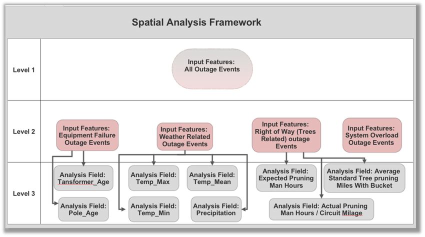
ISPRS
ISPRSInt.
Int.J.J.Geo-Inf. 2019,9,8,54
Geo-Inf.2020, x FOR PEER REVIEW 3 of
of 22
22
ISPRS Int. J. Geo-Inf. 2019, 8, x FOR PEER REVIEW 3 of 22
Figure1.1. U.S.
Figure U.S. reported
reportedpower
poweroutages
outagesby
byyear.
year.Source:
Source: Eaton’s
Eaton’s Blackout
BlackoutTracker
Tracker[16].
[16].
Figure 1. U.S. reported power outages by year. Source: Eaton’s Blackout Tracker [16].
Figure 2. U.S. reported power outages by cause in 2017. Source: Eaton’s Blackout Tracker [16].
Figure 2. U.S. reported power outages by cause in 2017. Source: Eaton’s Blackout Tracker [16].
Figure 2. U.S. reported power outages by cause in 2017. Source: Eaton’s Blackout Tracker [16].
After looking into the Eaton’s Blackout Tracker and other similar reports that investigate
After looking
power-outage into thewe
incidents, Eaton’s Blackout
identified Tracker
three key and otherunderlying
factors similar reports
these that investigate
outages power-
(Figure 3):
After
outage lookingwe
incidents, intoidentified
the Eaton’s Blackout
three key Tracker
factors and other these
underlying similar reports(Figure
outages that investigate
3): (1) power-
hardware
(1) hardware and technical failures, (2) environment-related, and (3) operation-related failures.
outage incidents,
and Environment-related
technical we identified
failures, three key factors
(2)incidents
environment-related, andunderlying
(3)portion these outages
operation-related (Figure 3): (1) hardware
failures.
comprise the largest of power-outage causes. Environment-
and technical failures,
Environment-related (2) environment-related,
incidents comprise andthe(3) operation-related
largest portion failures.
of power-outage causes.
related incidents can be classified into three distinct categories: weather, wildlife, and trees. Wisconsin
Environment-related
Environment-related incidents
incidents can be comprise into
classified thethree
largest portion
distinct of power-outage
categories: weather, causes.
wildlife, and
Public Service [17] delineated the weather-related causes of power outages; a 2005 study by Davies
Environment-related
trees. Wisconsin Public incidents
Service can
[17] be classifiedthe
delineated intoweather-related
three distinct categories:
causes of weather,
power wildlife,
outages; a and
2005
Consulting for the Edison Electric Institute stated that 70% of power outages in the United States
trees.
study Wisconsin
by Davies Public
Consulting Service
for [17] delineated
the Edison the weather-related
Electric causes
70%ofofpower outages; ain2005
are weather-related [18]. Kenward and Raja [19]Institute
analyzedstated that
power-outage power
data outages
over a 28-year the
study
United by Davies
States are Consulting for
weather-related the Edison
[18]. Electric
Kenward Institute
and Raja stated
[19] that
analyzed70% of power
power-outage outages
data in thea
over
period and pointed out that between 2003 and 2012, 80% of all outages were caused by weather.
United
28-yearStates
period areandweather-related
pointed [18].between
out that Kenward andand Raja2012,
[19] analyzed
of allpower-outage data overby a
Similarly, Campbell [20] highlighted the damage 2003to the electrical 80%caused
grid outages
by seasonalwere caused
storms, rain,
28-year
weather. period and pointed out that between 2003 and 2012, 80% of all outages
Similarly, Campbell [20] highlighted the damage to the electrical grid caused by seasonal were caused by
and high winds.
weather.
storms, Similarly,
rain, and Campbell
winds. [20] highlighted the damage to the electrical grid caused by seasonal
According to high
the President’s Council of Economic Advisers and the U.S. Department of Energy’s
storms, rain, andtohigh winds.
OfficeAccording
of Electricitythe President’s
Delivery CouncilReliability
and Energy of Economic[3], Advisers and theisU.S.
severe weather the Department
leading causeofof Energy’s
power
Office of Electricity Delivery and Council
According to the President’s of Economic
Energy Reliability [3],Advisers and the is
severe weather U.S.
theDepartment
leading causeof Energy’s
of power
Office of Electricity Delivery and Energy Reliability [3], severe weather is the leading cause of power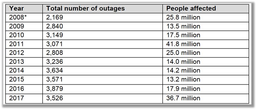
ISPRS Int. J. Geo-Inf. 2020, 9, 54 4 of 22
ISPRS Int. J. Geo-Inf. 2019, 8, x FOR PEER REVIEW 4 of 22
outages
outages in in the
the United
United States.
States. “Between
“Between 2003 2003 and
and 2012,
2012, an
an estimated
estimated 679679 widespread
widespread power
power outages
outages
occurred
occurred due to severe weather” [3] (p. 3). Likewise, annual costs changed significantly and
due to severe weather” [3] (p. 3). Likewise, annual costs changed significantly and were
were
greater
greater due
due to to ofof major
major storms
storms such
such asas Hurricane
Hurricane IkeIke in
in 2008. “Data from
2008. “Data from the U.S. Energy
the U.S. Energy Information
Information
Administration
Administration show show that
that weather-related
weather-related outages
outageshave
have increased
increasedsignificantly
significantlysince
since1992”
1992”[3][3](p.
(p. 8).
8).
In addition to weather, other external forces cause power outages.
In addition to weather, other external forces cause power outages. Falling tree branches, forFalling tree branches,
for example,
example, is another
is another important
important cause
cause forforpower
powerdisruption
disruption[21].
[21].Animals
Animalscoming
coming into
into contact
contact with
with
power lines, such as large birds, are also important culprits of power outage in
power lines, such as large birds, are also important culprits of power outage in the United States the United States [16].
[16].
Furthermore,
Furthermore, human-error
human-error incidents
incidents cause
cause power
power outages.
outages. Chayanam
Chayanam [7] [7] indicated
indicated that
that training
training isis
essential for technicians and staff to battle outages with proper maintenance
essential for technicians and staff to battle outages with proper maintenance procedures. procedures.
Figure 3. Causes of Power Failure/Prepared by Vivian
Vivian Sultan/Date
Sultan/Date Printed
Printed 77 January
January 2018.
2018.
Interrupted
Interruptedpower
powersupply
supplyis isnonolonger deemed
longer deemed a mere inconvenience.
a mere inconvenience.As theAs duration and spatial
the duration and
extent
spatialofextent
electricity-system outages outages
of electricity-system increase,increase,
costs and inconvenience
costs grow. Critical
and inconvenience grow. social services
Critical social
such as medical
services such ascare, police,
medical andpolice,
care, other andemergency services and
other emergency communications
services systems depend
and communications on
systems
electricity
depend ontoelectricity
function toat function
a minimum at a level.
minimumFailures
level.can bring about
Failures can bringcatastrophic outcomes,outcomes,
about catastrophic and lives
can
andbe lost.can
lives Grid
be reliability
lost. Grid is an area of
reliability is research that
an area of will help
research better
that willexplain the causes
help better explainofthe
outages
causesand
of
prescribe interventions that will improve the reliability of the smart grid.
outages and prescribe interventions that will improve the reliability of the smart grid. In thisIn this manuscript, we use
various spatial
manuscript, weanalytics toolsspatial
use various to investigate
analytics U.S. power
tools concerns and
to investigate U.S.topower
answer the research
concerns and toquestion:
answer
How may spatial
the research analytics
question: Howenhance
may spatial our understanding
analytics enhance of power outages?
our understanding of power outages?
To
To date,
date, there
there are
are several
several studies
studies thatthat delve
delve into
into several
several causes
causes of offailure.
failure. For
For instance,
instance, Reed
Reed
evaluated how powerpower delivery
delivery system
system dealtdealt with
with hurricanes
hurricanes [22].
[22]. Sun
Sun et
et al.
al. discussed
discussed social
social media
media
data in detecting
detecting power
power outages
outages [23]
[23] and
and Guven
Guven et et al.
al. discussed how a GIS could help to analyze an
electric
electric distribution
distributionnetwork
network[24].
[24].These
Thesestudies
studiesshow
showthatthatthere
thereisisa apalpable
palpableinterest
interestininusing
usingGIS inin
GIS a
data-driven
a data-driven wayway
to deal with with
to deal powerpower outages. Our research
outages. is different
Our research and noveland
is different in that we in
novel provided
that we a
general framework to help researchers and practitioners deal with the multitude
provided a general framework to help researchers and practitioners deal with the multitude of data of data in analyzing
power outagespower
in analyzing and integrated
outages and several outage events
integrated severaltooutage
detect events
regionstowhere
detect outage
regionsevents should
where outagebe
investigated
events should further.
be investigated further.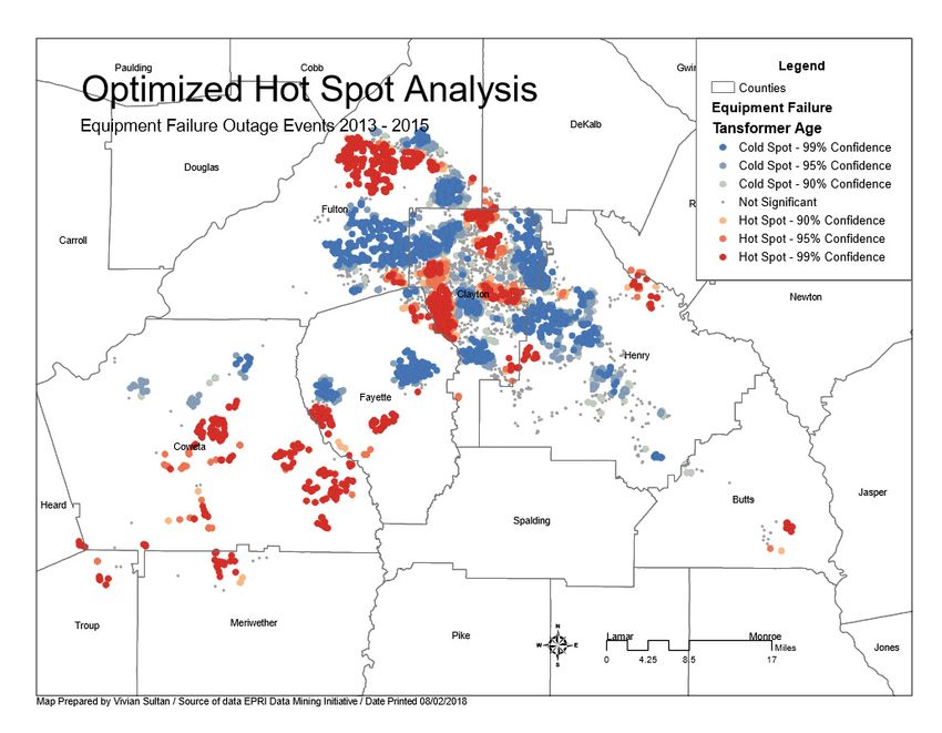
ISPRS Int. J. Geo-Inf. 2019, 8, x FOR PEER REVIEW 5 of 22
ISPRS Int. J. Geo-Inf. 2020, 9, 54 5 of 22
3. Data Selection and Acquisition
3. Data Selection and Acquisition
3.1. Infrastructure Data
3.1. Infrastructure Data Research Institute (EPRI) data repository includes the primary datasets we
The Electric Power
usedThe to Electric
conduct Power
this analysis.
ResearchThe datasets
Institute include
(EPRI) data from includes
data repository advanced themetering
primary systems,
datasets
supervisory control, and data acquisition (SCADA) systems,
we used to conduct this analysis. The datasets include data from advanced metering geospatial information systems (GIS),
systems,
outage-management systems (OMS), distribution-management systems
supervisory control, and data acquisition (SCADA) systems, geospatial information systems (GIS),(DMS), asset-management
systems, work-management
outage-management systems,distribution-management
systems (OMS), customer-information systems, systems and
(DMS), intelligent electronic-
asset-management
device databases. Access to datasets was provided as part of EPRI’s data-mining
systems, work-management systems, customer-information systems, and intelligent electronic-device initiative to provide
adatabases.
test bed for datatoexploration
Access datasets wasand innovation
provided as partand to solve
of EPRI’s the top challenges
data-mining initiative tofaced by the
provide utility
a test bed
industry [25].
for data exploration and innovation and to solve the top challenges faced by the utility industry [25].
When combined with
When combined clever analytical
with clever analytical techniques,
techniques, data
data provide
provide the potential to
the potential to transform
transform thethe
world into
world into aa smarter
smarterworld,
world,wherewherethe prevention
the prevention of of
power
power outages
outagesmaymaybecome
become a true reality,
a true not
reality,
merely
not merely a prediction. The SCADA/OMS/DMS archives at a power utility offer the required data to
a prediction. The SCADA/OMS/DMS archives at a power utility offer the required data to
identify
identify the
the parts
parts of
of the
the system
system that
that contribute
contribute most
most to
to overall
overall system
system downtime.
downtime. OMS, OMS, for for example,
example,
provides the
provides the data
data needed
needed to to calculate
calculate measurements
measurements of of system
system reliability.
reliability. OMS
OMS also
also provide
provide historical
historical
data
data that can be mined to find common causes, failures, and damages. Since OMS have become
that can be mined to find common causes, failures, and damages. Since OMS have become moremore
integrated with other operational systems such as GIS at the utility side, analysis
integrated with other operational systems such as GIS at the utility side, analysis has become more has become more
feasible, so this
feasible, so this research
research maymay aim
aim toto improve
improve gridgrid reliability.
reliability.
In
In general, EPRI’s data consist of one main GIS data
general, EPRI’s data consist of one main GIS file, where
data file, where this
this data
data isis linked
linked with
with seven
seven
databases withinthe
databases within the EPRI’s
EPRI’s information
information systems.
systems. WhileWhile somearelinks
some links basedareon based
uniqueon keyunique key
association,
association, several are linked spatially, via latitude and longitude. For example,
several are linked spatially, via latitude and longitude. For example, the GIS data can be linked with the GIS data can be
linked with the outage management system allowing for the analysis
the outage management system allowing for the analysis of the root cause of outages. of the root cause of outages.
3.2. Weather
Weather Data
1. Georgia
Georgiaspatial
spatialdata
datainfrastructure
infrastructure(GaSDI)
(GaSDI)andandthe
theGeorgia
Georgia GIS
GIS Clearinghouse
Clearinghouse is the data source
for
forthe
themonthly
monthlytemperature
temperatureandandprecipitation
precipitationdata
data we
we employed
employed in
in this
this study. “This dataset
contains
contains contours that represent the average monthly temperatures (1960–1991) for
contours that represent the average monthly temperatures (1960–1991) for the
the state of
Georgia
Georgia[and]
[and]display
displayappropriate
appropriateatatleast
leastat
atregional
regional scales
scales and
and above”
above” [26]. The
The data
data repository
repository
isisdisplayed in Figure 4.
displayed in Figure 4.
Figure 4.4. Monthly
Monthly Temperature Precipitation Data
Temperature and Precipitation Data Files.
Files. Source: Georgia
Georgia Spatial
Spatial Data
Infrastructure [26].
2. The
TheNational
NationalOceanic
Oceanicand
andAtmospheric
AtmosphericAdministration
Administrationwebsite
website(NOAA)
(NOAA) is
is the
the data
data source for
the
the storm and storm
storm events and stormdetails.
details.The
Thelink
link to the
to the NOAA
NOAA StormStorm Events
Events Database
Database is
is https:
//www.ncdc.noaa.gov/stormevents/. According
https://www.ncdc.noaa.gov/stormevents/. According to National
to NOAA’s NOAA'sCenters
National Centers for
for Environmental
Environmental Information [27], this database contains records used to create the official NOAA
Storm Data publication, detailing: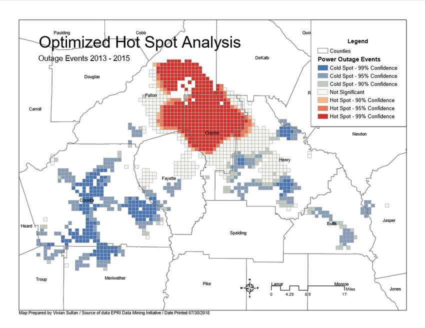
ISPRS Int. J. Geo-Inf. 2020, 9, 54                                                                            6 of 22

       Information [27], this database contains records used to create the official NOAA Storm Data
       publication, detailing:

       a.      The event of storms and other noteworthy weather phenomena;
       b.      Odd, scarce, weather phenomena that generate media attention; and
       c.      Other important meteorological events, such as record maximum or minimum temperatures
               or precipitation that occurs in connection with another event.

4. Methodology
      After the data has been obtained, preliminarily, data should be checked for inconsistencies, errors,
and omissions. Since this type of analytical project requires data to be analyzed spatially, any tool
used needs to be suitable for location analytics. One such tool is the ArcGIS platform, provided by the
Environmental Systems Research Institute (ESRI). Therefore, we opt to use this tool as a demonstration
of the analytical framework that others could adopt. In addition, the analytical framework needs a
way to make sure that the steps are reusable. Thus, the ModelBuilder tool in the ArcMap software is
utilized to create three models that could be exported and use in other similar analyses.
      The following subsections detailed the creation of the geodatabase to store all acquired data, and
the necessary steps to combine, sort, clean, and integrate data to arrive at the final processed sets of
data, ready for analysis.

4.1. Data Preparation
     First, we crated one geodatabase where all related data will reside with the WGS 1984 map
projection, suitable for the study site in Georgia, United States. The geodatabase was then fed with all
the aforementioned data and more general data, including (1) the imported data files from the EPRI’s
data repository, (2) Georgia’s Topologically Integrated Geographic Encoding and Referencing (TIGER)
road shapefile, (3) 2010 Georgia’s county shapefile, (4) NOAA’s storm and storm detail maps from
2013 to 2015, (5) 48 unzipped weather shapefiles, monthly temperatures, and precipitation data from
GaSDI and the Georgia GIS Clearinghouse (four total files showing the maximum, minimum, and
average temperature and the precipitation for each month of the year).
     Second, we perused the outage data, and realizing that about 5% of the data (3992 records out of
80,839 records) were not spatially-enabled, we excluded them from the analysis. The final outage data
has 76,848 records. Then, for each record, we create dummy variables to indicate the type of outage.
Overall, there are four major types of outages have been identified: right of way, weather, equipment
failure, and system overload, as shown in Table 1. With each of the outage events, we iteratively
separate each outage into its own map layer. To associate the outages events, we utilize the average
nearest-neighbor to identify the likelihood of data-forming clusters throughout the study sites.

                                 Table 1. Four types of outages and their associate events.

                 Outage Type                                     Outage Events
                 Right of Way         Wind/Tree, Limb online, Tree Fell on Line, Tree Grew into Line, Vines
                    Weather                            Wind, Ice, Major Storm, Lightning
                  Equipment                              Failed in Service, Deterioration
              System Overload                       Thermal Overload, Overload, Load Shed

     Third, to prepare the data, we convert the date time field in the NOAA’s storm and storm event
datasets into the day of the year so that the date component in all the data is synchronized.
     Fourth, after setting up the data, we create data processing steps via the ArcMap ModelBuilder
tool so that the steps could systematically go through all weather data layers within the geodatabase.
We separate the steps into three models. The result of the models is an outage table with an additional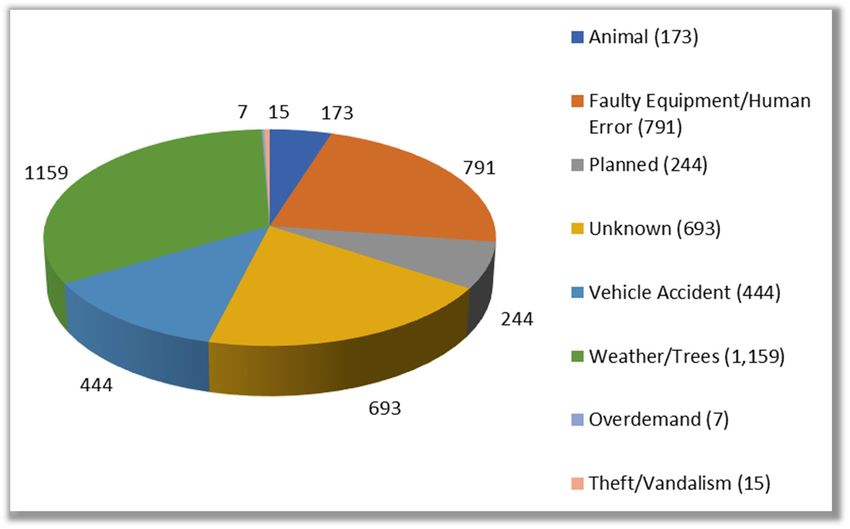
ISPRS Int. J. Geo-Inf. 2020, 9, 54 7 of 22
48 columns (four columns for each month displaying the maximum, mean, and minimum temperature,
ISPRS
and Int. J. Geo-Inf.
another field2019, 8, x FOR
for the PEER REVIEW
precipitation for each outage event location). 7 of 22
4.1.1. Interpreting
4.1.1. Interpreting aa Model
Model in
in ModelBuilder
ModelBuilder
First, ModelBuilder
First, ModelBuilder isis aagraphical
graphicalworkflow
workflowthat thathelps
helpsto to
streamline
streamlineall all
geoprocessing
geoprocessing steps. All
steps.
input
All data,
input geoprocessing
data, geoprocessing tools, intermediary
tools, intermediaryresulting
resultingdata,
data,andandoutput
output data
data are displayed with
are displayed with
specificcolors
specific colorsand
andshapes.
shapes. The
The blue
blue oval
oval in
in the
the ModelBuilder
ModelBuilder depictsdepicts input
input data
data and
and the
the green
green oval
oval
depictsresultant
depicts resultantdata.
data. The
The teal
teal oval
oval depicts
depicts resultant
resultant value,
value, the
the rectangle
rectangle shows
shows aa specific
specific processing
processing
tool, and the hexagon depicts an iterator, which is used to go through a specific list
tool, and the hexagon depicts an iterator, which is used to go through a specific list of items within of items withinaa
repository. The arrows are used to connect each component of a model within
repository. The arrows are used to connect each component of a model within ModelBuilder. As ModelBuilder. As aa
convention,the
convention, themodel
modelworkflow
workflowstarts
startsfrom
fromleftlefttotoright.
right.
4.1.2.
4.1.2. Model
Model 11
Model
Model1,1,depicted
depictedin in
Figure 5, shows
Figure that that
5, shows the workflow starts starts
the workflow from selecting each weather
from selecting feature
each weather
iteratively, and spatially
feature iteratively, joins with
and spatially thewith
joins combined outageoutage
the combined data file.
dataThis
file.results in a new
This results in afeature that
new feature
contains data from
that contains each weather
data from file and
each weather filethe
andoutage eventevent
the outage file. file.
Figure 5. ArcMap ModelBuilder (Model 1) to spatially join the outage events with the weather data.
Figure 5. ArcMap ModelBuilder (Model 1) to spatially join the outage events with the weather data.
4.1.3. Model 2
4.1.3. Model 2
The results of the Model 1 are 48 files corresponding to each weather dataset combined with the
outageThe results
events. of the Model
Therefore, 1 are
Model 2 is48 filestocorresponding
used to each
rename the output fieldweather datasettocombined
appropriately reflect thewith the
month
outage
and typeevents. Therefore,
of weather Model max,
data (whether 2 is used to rename
min, mean the output
temperature, field appropriately
or average precipitation).toThereflect the
process
month and type of weather data
of Model 2 is displayed in Figure 6. (whether max, min, mean temperature, or average precipitation).
The process of Model 2 is displayed in Figure 6.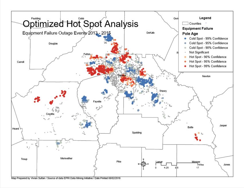
ISPRSInt.
ISPRS Int. J.J. Geo-Inf.
Geo-Inf. 2020,
2019,9,
8,54
x FOR PEER REVIEW 88 of 22
22
ISPRS Int. J. Geo-Inf. 2019, 8, x FOR PEER REVIEW 8 of 22
Figure
Figure 6.
6. ArcMap
ArcMap ModelBuilder
ModelBuilder (Model
(Model 2)
2) to
to rename
rename the
the output
output field
field (contour
(contour field)
field) from Model 1.
from Model 1.
Figure 6. ArcMap ModelBuilder (Model 2) to rename the output field (contour field) from Model 1.
4.1.4.
4.1.4. Model
Model 33
4.1.4. Model 3
The
The last
last model,
model, Model
Model 33 (Figure
(Figure 7),
7), made
made sure
sure that
that the
the processed
processed data
data from
from the
the previous
previous two
two
models
models The last model,
contained
contained Model
ininone 3 (Figure
oneunified
unified feature 7),
feature made
layer. For
layer. sure
each
For that
each thethe
of the
of processed
48 joined data from
features,
48 joined the the
features, previous
model selects
model two
the
selects
models
the contained
appropriate infield
join field
appropriate join one and
and unified feature
iteratively layer.
joinsjoins
iteratively allFor
all data each
into
data theof
into theoutage
outage
the 48event
joined features,
layer. the model selects
layer.
event
the appropriate join field and iteratively joins all data into the outage event layer.
Figure 7. ArcMap ModelBuilder (Model 3) to join outage-events data with the 48 fields of weather data.
Figure 7. ArcMap ModelBuilder (Model 3) to join outage-events data with the 48 fields of weather
Figure 7. ArcMap ModelBuilder (Model 3) to join outage-events data with the 48 fields of weather
data.
Fifth, after the data is processed through the ModelBuilder, we continue to enrich the data by
data.
creating four additional columns to the outage map attribute table to show the weather data for each
Fifth, after the data is processed through the ModelBuilder, we continue to enrich the data by
outage event, considering the month of the year. For each outage event, we showed data for the
Fifth,
creating after
four the datacolumns
additional is processed
to thethrough the ModelBuilder,
outage map attribute table we continue
to show to enrichdata
the weather the for
data by
each
maximum, mean, and minimum temperature, and precipitation. We followed this step by joining
creatingevent,
outage four additional
consideringcolumns to theofoutage
the month mapFor
the year. attribute table to event,
each outage show thewe weather
showed datadataforforeach
the
three additional data sources to the combined layer, namely the storm event and storm event details
outage event,
maximum, considering
mean, the month
and minimum of the year.
temperature, andFor each outage
precipitation. We event, we showed
followed this stepdata for the
by joining
via the data transformation in the processing steps. Additionally, we added the following forestry
maximum,
three mean,
additional andsources
data minimum temperature,
to the and precipitation.
combined layer, namely the storm We event
followed
andthis
stormstep by joining
event details
data, showing how EPRI has maintained its infrastructure: “Forestry Expected Pruning Man Hours,”
three
via additional
the data sourcesintothe
data transformation theprocessing
combined layer,
steps. namely the storm
Additionally, we event
addedandthestorm eventforestry
following details
“Average Standard Tree Pruning Miles with Bucket,” “Average Mechanical Tree Pruning Miles,”
via the data transformation in the processing steps. Additionally, we added the
data, showing how EPRI has maintained its infrastructure: “Forestry Expected Pruning Man Hours,” following forestry
“Average Climbing Tree Pruning Miles,” and “Actual Pruning Man Hours/Circuit Mileage.” Finally,
data, showing
“Average how EPRI
Standard Tree has maintained
Pruning Miles its infrastructure:
with “Forestry
Bucket,” “Average Expected Pruning
Mechanical Man Hours,”
Tree Pruning Miles,”
we derived several equipment data, specifically transformer’s age and pole’s age to show how long a
Standard Tree
“Average Climbing TreePruning
PruningMiles,”
Miles with Bucket,”Pruning
and “Actual “Average ManMechanical TreeMileage.”
Hours/Circuit Pruning Finally,
Miles,”
transformer and pole last since its first installation to its demise, respectively.
“Average Climbing Tree Pruning Miles,” and “Actual Pruning Man Hours/Circuit
we derived several equipment data, specifically transformer’s age and pole’s age to show how long Mileage.” Finally,
awe derived several
transformer equipment
and pole last sincedata, specifically
its first transformer’s
installation agerespectively.
to its demise, and pole’s age to show how long
a transformer and pole last since its first installation to its demise, respectively.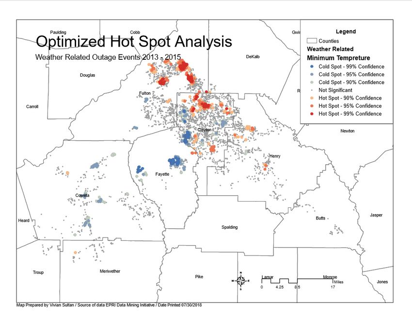
ISPRS Int. J. Geo-Inf. 2020, 9, 54                                                                         9 of 22

4.2. Analysis Framework
     After making sure that data are properly processed, we start the analysis process. The analysis
consists of two types: non-spatial and spatial. First, the non-spatial analysis follows the traditional
exploratory and confirmatory analysis. For instance, we explore the statistical relationships within
the data using descriptive statistics and correlation analysis. Within this step, other analysis could be
included, namely factor analysis or exploratory data analysis. This capability does not exist in the
ArcGIS platform, so we opt to use SPSS for this task. In fact, any statistical tool would suffice. This step
essentially provides an initial understanding of the data and how each component of the data could
relate to one another in a non-spatial way.
     Subsequently, a spatial analysis is conducted, showing how the outage could be analyzed through
location analytics. In this instance, we select two analysis methods: hotspot analysis to show an initial
analysis through space and emerging hotspot analysis to show how outage events are related to one
another through space and time.

5. Results and Findings

5.1. Initial Exploration
     Initial data exploration indicated inadequate data for analysis and many null fields, as shown
in Table 2. For example, the asset management folder showed inspection data for only two types
of equipment. As for the age of asset data embedded in the GIS maps, analyses showed that “last
date installed” and “original date installed” fields for equipment, but these were mostly null values.
For instance, of the 4600 records for switches, only 106 records showed original date installed, which is
equivalent to 2% of the total records. Thus, we decided to use pole-age data as a proxy for the rest of
the equipment data in the analysis.
     Not all files in the data set appeared useful considering the scope of this project work. For example,
the Jets data file is about the field jobs. Another example is the circuit “load” data that do not include
longitude/latitude data or any other georeferencing method to bring into ArcGIS. “load” data appeared
to be overall feeder data and because distribution feeders are highly branched, data are not useful to
draw conclusions on which branch is loaded and which is not. As for other data collections, such as
SCADA data files, research indicated that it is only helpful if we need to dig into one of the operations
that caused outage events.

                                           Table 2. Power-outage cause category.

             Outage Type             Percent of Outage Events Duration    Percent of Outage Events Count
              Equipment                           10.19%                              6.03%
             Right of Way                         12.35%                              7.02%
           System Overload                         1.00%                              0.52%
               Weather                            16.97%                              4.57%
                Total                             40.51%                             18.13%

5.2. Descriptive Statistics
      In the final resultant dataset, the data contains the duration of the outage event, the number of
notifications from the customer, the mean temperature, the precipitation, several forestry data attributes
concerning tree pruning and maintenance, and age of the equipment, namely transformers and poles.
The descriptive statistics in Table 3 show that there is a wide range of values between each data point.
For instance, with the outage event customer calls, the mean is at 11.19, but the standard deviation is
85.07, with the max of 4888. This shows that, while there are many low call volumes, there are several
instances whereby the notifications are numerous, thus skewing the data. It is also interesting to note
that the equipment could fail as early as three years, and the transformers last up to eight years while
poles can sustain for 93 years until succumbing to outage events.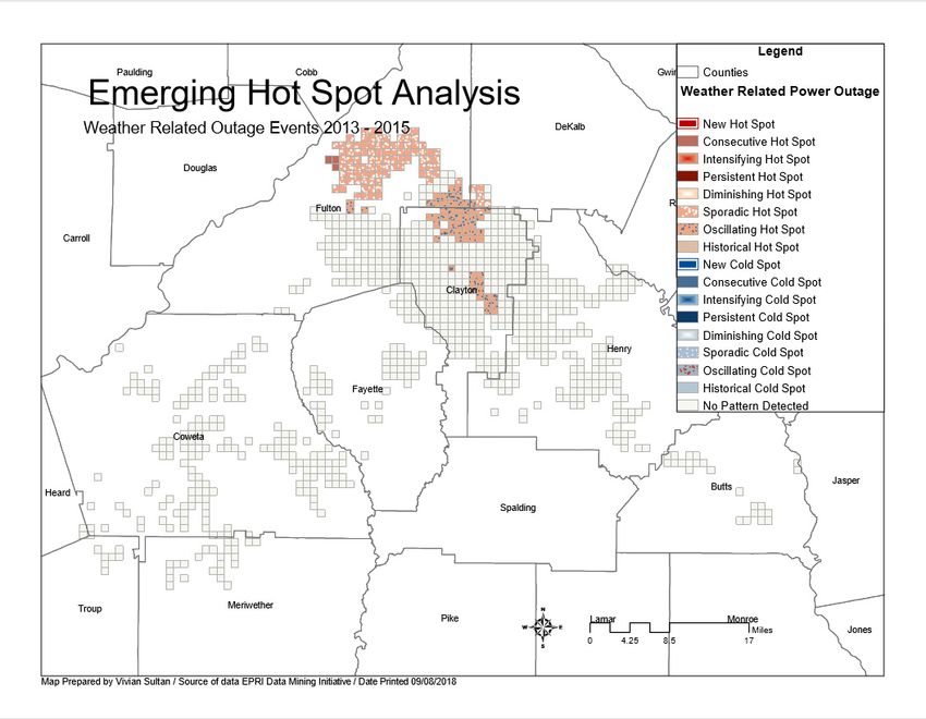
ISPRS Int. J. Geo-Inf. 2020, 9, 54                                                                           10 of 22

                                     Table 3. Descriptive statistics of study variables.

                                      Variable.                             M        SD      Min     Max
                           Outage event duration                          89.15     204.81     0     3589
                         Outage event customer calls                       11.18     85.07     0     4888
                             Temperature (mean)                           62.52      13.72   40.25   80.75
                                 Precipitation                             4.29       0.66    2.8     5.80
                    Forestry expected pruning man hours                   858.01    882.24     0     3300
               Average standard tree pruning miles with bucket             6.63       6.48     0     20.49
                   Average mechanical tree pruning miles                    3.00      2.94     0     9.28
                    Average climbing tree pruning miles                    0.75       0.73     0      2.32
                   Actual pruning man hours/circuit mile                  42.18      36.80     0      157
                               Transformer age                             4.50       1.86     3        8
                                   Pole age                               23.90      16.76     3       93
                                                      Note: n = 76,847.

5.3. Correlation Results
       To further explore the relationships between the variables, we ran the correlation analysis.
The result is shown in Table 4. The correlation matrix shows that the duration of an outage event is
significantly correlated with most of the variables in the dataset except whether the event is part of the
forestry management route. Outage event duration is negatively correlated with temperature. While
the relationship is significant, it is not strong. As for the number of calls from the customer, a somewhat
opposite result could be observed. There are only four variables that are statistically significant with
outage event customer calls: forestry management, actual pruning staff hours/circuit mile, transformer
age, and pole age. In addition, the relationships are trivial.
       It is interesting to observe that pole age is statistically significant with all other variables, indicating
the importance of the age of the pole when it comes to perusing outages data. However, the relationship
is minimally correlated. Meanwhile, transformer age is also statistically significant with all variables
except temperature. Intriguingly, there is no relationship between transformer age and temperature.
It is also expected to see that the forestry-related variables are highly positively correlated, with a high
statistical significance power.
       Overall, the correlation matrix shows that there are notable relationships between the variables.
However, despite their statistical significance, the correlation relationships are marginal. Therefore,
this creates a need to analyze data spatially. In the next section, we present the spatial analysis
framework, and then perform several analyses to highlight the importance of incorporating a spatial
component into any analysis task.
ISPRS Int. J. Geo-Inf. 2020, 9, 54 11 of 22
Table 4. Correlation results.
Average
Outage Forestry Average Average Actual
Outage Storm Forestry Standard
Event Temperature Expected Mechanical Climbing Pruning Staff Transformer Pole
Variable Event Event (1 Precipitation Management Tree-Pruning
Customer (mean) Pruning Tree-Pruning Tree-Pruning Hours/Circuit Age Age
Duration = yes) (1 = yes) Miles with
Calls Staff Hours Miles Miles Mile
Bucket
Outage event duration 1.00
Outage event
0.09 ** 1.00
customer calls
Storm event (1 = yes) 0.08 ** 0.01 1.00
Temperature (mean) −0.13 ** 0.01 0.14 ** 1.00
Precipitation 0.08 ** 0.00 −0.06 ** −0.37 ** 1.00
Forestry management
0.01 −0.02 ** −0.01 0.00 −0.03 ** 1.00
(1 = yes)
Forestry expected
0.01 ** 0.00 0.00 0.00 −0.02 ** 0.77 ** 1.00
pruning staff hours
Average standard
tree-pruning miles 0.01 ** 0.00 0.00 0.00 −0.02 ** 0.81 ** 0.96 ** 1.00
with bucket
Average mechanical
0.01 ** 0.00 0.00 0.00 −0.02 ** 0.81 ** 0.96 ** 1.00 1.00
tree-pruning miles
Average climbing
0.01 ** 0.00 0.00 0.00 −0.02 ** 0.81 ** 0.96 ** 1.00 ** 1.00 1.00
tree-pruning miles
Actual pruning staff
0.01 * −0.01 ** −0.01 −0.01 ** −0.02 ** 0.91 ** 0.85 ** 0.79 ** 0.79 ** 0.79 ** 1.00
hours/circuit mile
Transformer age 0.01 * 0.01 ** 0.01 ** 0.00 0.02 ** −0.13 ** −0.11 ** −0.12 ** −0.12 ** −0.12 ** −0.11 ** 1.00
Pole age 0.02 ** −0.01 ** 0.02 ** −0.01 ** 0.03 ** 0.02 ** 0.04 ** 0.03 ** 0.03 ** 0.03 ** 0.03 ** −0.03 ** 1.00
NOTE: * p < 0.05; ** p < 0.01, two-tailed tests.ISPRS Int. J. Geo-Inf. 2020, 9, 54 12 of 22
5.4. Spatial Pattern Analysis in ArcGIS
Based on ArcGIS average nearest neighbor analyses reports displayed in Figure 8, the observed
mean distance is the largest between system-overload outage events (727 m) compared to
weather-related events (171 m), equipment failure (207 m), and right-of-way outage events (210 m).
Weather-related outage showed the shortest mean distance between events. A clustered pattern
appeared for all four outage-event types. Additionally, based on the analysis results, there is less
than 1% likelihood that this clustered pattern could be the result of random chance, indicating
statistical ISPRS
significance.
Int. J. Geo-Inf. 2019, 8, x FOR PEER REVIEW 12 of 22
Figure 8. ArcGIS average
Figure 8. ArcGIS nearest
average neighbor
nearest analyses
neighbor resultsforfor
analyses results four
four types
types of outages:
of outages: weather weather
(top (top
left), system overload
left), (top right),
system overload equipment
(top right), equipment(bottom and
left),and
(bottom left), right
right of way
of way (bottom
(bottom right). right).ISPRS Int. J. Geo-Inf. 2020, 9, 54 13 of 22
ISPRS Int. J. Geo-Inf. 2019, 8, x FOR PEER REVIEW 13 of 22
5.4.1.
5.4.1. Spatial
Spatial Analysis
Analysis Framework
Framework
We
Wedeveloped
developedthe thefollowing
followingframework
framework (Figure(Figure 9)9) to
toguide
guidethetheinvestigation
investigation and
and illustrate
illustrate the
the
various
various levels
levels of
ofanalysis.
analysis. AtAt the
the first
first level,
level, all
all features
features inin the
the outage
outage events
events are
are analyzed
analyzed toto provide
provide
aa general
general sense
sense ofof where
where inin space
space thethe clusters
clusters ofof outages
outages might
might be.be. As wewe get
get more
more refined
refined in
in the
the
granularity
granularityofofthe
thedata,
data,Level
Level22 indicates
indicates aa more
more specific
specific group
groupinput
input features,
features,namely
namelytypes
typesof
of outage
outage
events. this case,
events. In this case,there
thereare
arefour:
four:equipment
equipment failure,
failure, weather,
weather, right
right of of way,
way, and and system
system overload.
overload. As
As
thethe analysis
analysis drills
drills downdown to finer
to finer details,
details, Level
Level 3 approaches
3 approaches eacheach individual
individual feature
feature in each
in each typetype
and
and in turn,
in turn, provides
provides the analysis
the analysis for a particular
for a particular feature. feature.
Using thisUsing this framework,
framework, the subsequent
the subsequent sections
sections
provide provide the implementation
the implementation and theand the results
results of eachoflevel.
each level. Specifically,
Specifically, we useweoptimized
use optimized hot
hot spot
spot analysis
analysis forlevels
for all all levels
andand emerging
emerging hothot spot
spot analysis
analysis forforLevel
Level1 1and
andLevel
Level 2.
2. These
These are meant
meant toto
demonstrate
demonstratehow howsuch
suchaaframework
frameworkcould couldapply
applyto toother
othersimilar
similarscenarios.
scenarios.
Figure 9. Spatial Analysis Framework.
Figure 9. Spatial Analysis Framework.
5.4.2. Level 1 Spatial Analysis—Optimized Hot Spot Analysis
5.4.2. Level 1 Spatial Analysis—Optimized Hot Spot Analysis
Based on Level 1 of the spatial analysis framework, we used ArcGIS optimized hot spot analysis
tool toBased on Level
generate a map 1 of the spatial
(Figure 10) ofanalysis framework,
statistically we used
noteworthy ArcGIS
hot and coldoptimized
spots using hotthe
spot analysis
Getis-Ord
toolstatistic.
Gi* to generate a map
Since we did(Figure 10) of statistically
not identify an analysis noteworthy hot and
field, this tool cold spots
assessed using the Getis-Ord
the characteristics of the
input feature class (power outage events) to produce optimal results [27]. The tool showed one of
Gi* statistic. Since we did not identify an analysis field, this tool assessed the characteristics the
large
input feature class (power outage events) to produce optimal results [27]. The tool
area of hot spots in Clayton and Fulton County where power outage was statistically significant due to showed one large
area of hot
multiple spotsAs
causes. in Clayton and Fulton
for cold spots, County where
they appeared powersuch
in counties outage was statistically
as Coweta, mid andsignificant due
South Fayette,
to multiple causes. As for cold spots, they
Butts, North Meriwether, and a majority of Henry County. appeared in counties such as Coweta, mid and South
Fayette,
WithButts, Northcell
a polygon Meriwether,
size of 1319andm,athere
majority of Henry
are 1296 County.
weighted polygons on the study site. For each
With a polygon cell size of 1319 m, there are 1296
of the cells, there are an average of 59.29 incident counts, with weighted polygons on the deviation
the standard study site. of
For81.23.
each
of the cells, there are an average of 59.29 incident counts, with the standard
The minimum and maximum of incidents counts are 1 and 598, respectively. Correspondingly, deviation of 81.23. The
minimum
the optimal and maximumband
fixed-distance of incidents
based on the counts are distance
average 1 and 598,to 30respectively. Correspondingly,
nearest neighbors is 5738 m. There the
optimal fixed-distance band based on the average distance to 30 nearest neighbors
are 984 statistically significant output features, based on a false-discovery-rate correction for multipleis 5738 m. There
are 984and
testing statistically significant output
spatial dependence. features,only
Additionally, based on of
0.5% a false-discovery-rate
features had fewer than correction for multiple
eight neighbors.
testing and spatial dependence. Additionally, only 0.5% of features had fewer than eight neighbors.ISPRS Int. J. Geo-Inf. 2020, 9, 54 14 of 22
ISPRS Int. J. Geo-Inf. 2019, 8, x FOR PEER REVIEW 14 of 22
Figure 10. ArcGIS optimized hot-spot analysis Level 1 output map.
Figure 10. ArcGIS optimized hot-spot analysis Level 1 output map.
5.4.3. Level 1 Spatial Analysis—Emerging Hot Spot Analysis
5.4.3. Level 1 Spatial Analysis—Emerging Hot Spot Analysis
In addition to optimized hot spot analysis, emerging hot spot analysis is another candidate of
In addition
the type of spatialtoanalysis
optimized
thathot
couldspotbeanalysis, emerging
run. Emerging hot hot
spotspot analysis
analysis is another
is similar candidate
to optimized of
hot
the type
spot of spatial
analysis, with analysis
an addedthat could beof
dimension run. Emerging
time. hot spot
As a result, analysis
hot and cold is similar
spot to optimized
categories expandhotto
spot types,
new analysis, with annew,
including added dimension intensifying,
consecutive, of time. As a persistent,
result, hot and cold spotsporadic,
diminishing, categoriesoscillating,
expand to
newhistorical.
and types, including new, consecutive,
The categories are defined as intensifying,
follows: persistent, diminishing, sporadic, oscillating,
and historical. The categories are defined as follows:
• New: the most recent time step interval is hot/cold for the first time
• • New: the most
Consecutive: recent uninterrupted
a single time step intervalrunisofhot/cold
hot/coldfor the firstintervals,
time-step time comprised of less than
• 90%Consecutive: a
of all intervalssingle uninterrupted run of hot/cold time-step intervals, comprised of less than
90% of all intervals
• Intensifying: at least 90% of the time-step intervals are hot/cold, and becoming hotter/colder
• Intensifying: at least 90% of the time-step intervals are hot/cold, and becoming hotter/colder over
over time
time
• Persistent: at least 90% of the time-step intervals are hot/cold, with no trend up or down
• Persistent: at least 90% of the time-step intervals are hot/cold, with no trend up or down
• Diminishing: at least 90% of the time-step intervals are hot/cold and becoming less hot/cold
• Diminishing: at least 90% of the time-step intervals are hot/cold and becoming less hot/cold over
over time
time
• • Sporadic:
Sporadic:lesslessthan
than90%
90%of ofthe
thetime-step
time-stepintervals
intervalsare
arehot/cold
hot/cold
• • Oscillating:
Oscillating: the most recent time step interval is hot/cold,less
the most recent time step interval is hot/cold, lessthan
than90%
90%of ofthe
thetime-step
time-stepintervals
intervals
are
arehot/cold
hot/coldand anditithas
hasaahistory
historyofofreverse
reversefrom
fromhothottotocold
coldand
andvice
viceversa.
versa.
• • Historical:
Historical: at at least
least 90%
90% ofof the
the time-step
time-step intervals
intervals are
are hot/cold,
hot/cold, but
but the
the most
most recent
recent time-step
time-step
interval
intervalisisnot
not
The
Thefollowing
followingsection
sectionrecaps
recapsArcGIS
ArcGISemerging
emerginghot
hotspot analysis
spot results,
analysis and
results, thethe
and interpretation of
interpretation
the results.
of the results.
In Figure 11, the space–time cube aggregated 76,847 points into 6000 fishnet grid locations over
32 time-step intervals. Each location is 1319 m by 1319 m square. The entire space–time cube spansISPRS Int. J. Geo-Inf. 2020, 9, 54 15 of 22
ISPRS Int. J. Geo-Inf. 2019, 8, x FOR PEER REVIEW 15 of 22
In Figure 11, the space–time cube aggregated 76,847 points into 6000 fishnet grid locations over 32
time-step intervals.
an area 131,900 Each
m west tolocation
east andis79,140
1319 m mby 1319tomsouth.
north square. Thetime-step
Each entire space–time
interval iscube spans
1 month soanthearea
131,900 m west
entire time to east
period and 79,140
covered by themspace–time
north to south.
cubeEach
is 32time-step
months. interval is 1 month
Of the 6000 so the entire
total locations, 1296time
period covered by the space–time cube is 32 months. Of the 6000 total locations, 1296 (21.60%)
(21.60%) contain at least one point for at least one time-step interval. These 1296 locations comprise contain
at leastspace–time
41,472 one point for
binsatof
least one18,973
which time-step interval.
(45.75%) haveThese
point 1296 locations
counts comprise
greater than zero. 41,472 space–time
No statistically
bins of which
significant 18,973 or
increase (45.75%) have
decrease point counts
emerged greater
in point thanover
counts zero.time.
No statistically
The summary significant increase
of results is
or decrease emerged
displayed in Table 5. in point counts over time. The summary of results is displayed in Table 5.
Figure 11. ArcGIS Emerging Hot Spot Analysis Level 1.
Figure 11. ArcGIS Emerging Hot Spot Analysis Level 1.
Overall, the emerging hot spot analysis elucidates a more drill-down look at the cold and hot
Overall, the emerging hot spot analysis elucidates a more drill-down look at the cold and hot
spots observed in the optimized hot spot analysis. With the addition of time, another dimension,
spots observed in the optimized hot spot analysis. With the addition of time, another dimension, we
we can observe that there are many areas are persistent hot and cold spots, indicating where chronic
can observe that there are many areas are persistent hot and cold spots, indicating where chronic
issues and stability are respectively. Persistent hot spots cluster in the north west of Clayton county
issues and stability are respectively. Persistent hot spots cluster in the north west of Clayton county
while persistent cold spots can be found in Henry, Butte, Merriweather, Troup, Fayette, and Coweta
while persistent cold spots can be found in Henry, Butte, Merriweather, Troup, Fayette, and Coweta
counties. Thesespots
counties. These spotsindicate
indicatethat,
that,through
through90% 90%ofofthe
the time,
time, the
the locations
locations areare identified
identified as as
hothot
andand
cold spots consistently.
cold spots consistently. Furthermore,
Furthermore,there
thereare
aresome
someintensifying
intensifyinghothot spots
spots near
near north
north of Clayton
of Clayton andand
Fulton county, signifying a need for further investigation. In the west of Fayette county,
Fulton county, signifying a need for further investigation. In the west of Fayette county, we can find we can find
some oscillating cold spots, the locations where they used to be hot spots but have
some oscillating cold spots, the locations where they used to be hot spots but have now transitionednow transitioned
to cold spots.
to cold spots.These
Theseareare fascinating
fascinating because
because it could
it could be studied
be studied further
further to seetowhat
see what has supported
has supported the
the improvement of reducing outage events. Such understandings
improvement of reducing outage events. Such understandings could be used to improvecould be used to improve other
other
locations, especially those
locations, especially thosewhich
whichare areclassified
classifiedasaspersistent
persistenthot
hotspots
spotsandand intensifying
intensifying hot
hot spots.
spots.ISPRSInt.
ISPRS Int. J.J. Geo-Inf.
Geo-Inf. 2020,
2019, 9,
8, 54
x FOR PEER REVIEW 16 of 22
16 of 22
Table 5. Analysis summary of emerging hot spot level 1 results.
Table 5. Analysis summary of emerging hot spot level 1 results.
HOTCOLD
New HOT 0 0COLD
Consecutive
New 00 0 0
Intensifying
Consecutive 169
0 57 0
Persistent 169
Intensifying 86 29857
Diminishing 860
Persistent 16298
Sporadic 227
Diminishing 0 11316
Sporadic
Oscillating 227
37 17113
Oscillating
Historical 370 21 17
Historical 0 21
5.4.4. Level 2 Spatial Analysis—Optimized Hot Spot Analysis
5.4.4. Level 2 Spatial Analysis—Optimized Hot Spot Analysis
Based on Level 2 of the spatial analysis framework, we generated an additional four map layers
Based
(Figure 12)on Level
using the2 of the spatial
optimized hot analysis framework,
spot analysis tool by weconsecutively
generated an additional
selecting the four mapfeature
input layers
(Figure 12) usingoverload
classes “System the optimized hot spot
power outage analysis
events,” tool by consecutively
“equipment failure outage selecting
events,”the input feature
“weather related
classes
outage“System
events,” overload
and “right power
of way outage
outage events,”
events.”“equipment failure outage events,” “weather related
outage Theevents,”
map on andthe“right
top leftof way outage
of Figure 12events.”
indicated the outages based on system overload. There is
onlyTheone map
smallon the top
region leftsouth
in the of Figure 12 indicated
of Clayton countythe thatoutages basedas
is identified ona system
hot spot.overload. There is
The relationships
only
of allone small
other region
spots in the south ofsignifying
are insignificant, Clayton county that is identified
a uniformity in outage as a hotbased
events spot. The relationships
on system issues.
of
Asall other spots
a result, arespot
this hot insignificant, signifyingfurther
should investigate a uniformity
and making in outagesure events
to bringbased
downon system
the issues.
high level of
As a result, this hot spot should investigate
outages in this region due to system overloading. further and making sure to bring down the high level of
outagesTheinmapthis on
region dueright
the top to system overloading.
of Figure 12 provided the result of an optimized hot spot analysis for
The map
equipment on theAs
failure. topweright
can of Figure
see, there 12
is aprovided
large hotthe result
spot of aninoptimized
resided hot spotlocated
Clayton county, analysis in for
the
equipment
middle to the failure.
northAs ofwethecan see, there
county, is a large further
and extended hot spotnorth resided intoinFulton
Clayton county,
county. locatedlike
It seems in the
the
middle
equipment to the north
used of the
in this county,
region andfail
would extended further
faster than the north
rest ofintothe Fulton county. Itmore
state. Therefore, seemsresources
like the
equipment used intothis
should be placed region check
routinely wouldand fail maintain
faster than the rest
a high level of of
theoperationality
state. Therefore, andmore resources
redundancy to
should
make surebe placed
that the to routinely
equipmentcheck andismaintain
failure brought adown.high level of operationality
Furthermore, there areand redundancy
several cold spots to
make
observedsureinthat
thisthe
map. equipment failure isHenry
More specifically, brought down.
county hasFurthermore,
a cold spot in there are several
the north, cold spots
and sporadic cold
observed
spots around in this map. and
middle More specifically,
south HenryAdditionally,
of the county. county has a Coweta cold spotcounty
in the has
north, and sporadic
a cluster cold
of cold spots
spots
in thearound
southeastmiddlewhileandMeriwether
south of thecountycounty. hasAdditionally,
a cold spot Coweta
in thecounty
north.has a cluster
These locationsof cold spots
provide
in the southeast
another while Meriwether
good location county hasThese
for investigation. a cold spot in the north.
investigations Thesereveal
could locations
bestprovide
practicesanother
and
good location
standards thatfor investigation.
could These investigations
be used to improve the equipment could reveal
failure best
event inpractices
the hot spotandlocations.
standards that
couldCoincidently,
be used to improve the equipment
the optimized hot spot failure event
analysis forinweather
the hot spot locations.
(bottom left of Figure 12) is almost
Coincidently,
identical with thethe oneoptimized
for equipmenthot spot analysis
failure. Thisforfinding
weathershould (bottom beleft of Figure 12)
investigated is almost
further, and
identical
authoritieswith the one
could for equipment
formulate a plan to failure.
battleThis finding
weather should
related be investigated
issues while also further, and authorities
addressing equipment
could
failureformulate
ones. a plan to battle weather related issues while also addressing equipment failure ones.
Figure 12. Cont.You can also read