The Sleep Loss Insult of Spring Daylight Savings in the US Is Observable in Twitter Activity - Research Square
←
→
Page content transcription
If your browser does not render page correctly, please read the page content below
The Sleep Loss Insult of Spring Daylight Savings in the US Is Observable in Twitter Activity Kelsey Linnell ( klinnell@uvm.edu ) Vermont Complex Systems Center, UVM Michael Arnold Vermont Complex Systems Center, UVM Thayer Alshaabi Vermont Complex Systems Center, UVM Thomas McAndrew University of Massachusetts Amherst Jeanie Lim MassMutual Data Science Peter Sheridan Dodds Vermont Complex Systems Center, UVM Christopher M. Danforth Vermont Complex Systems Center, UVM Research Article Keywords: Sleep loss, heart disease, diabetes, cancer, Daylight Savings Time Posted Date: February 18th, 2021 DOI: https://doi.org/10.21203/rs.3.rs-198809/v1 License: This work is licensed under a Creative Commons Attribution 4.0 International License. Read Full License
The sleep loss insult of Spring Daylight Savings in the US is
observable in Twitter activity
Kelsey Linnell1* , Michael Arnold 1 , Thayer Alshaabi1 , Thomas McAndrew2 , Jeanie
Lim3 , Peter Sheridan Dodds1 , Christopher M. Danforth1 ,

1 Computational Story Lab, Vermont Complex Systems Center, MassMutual Center of
Excellence for Complex Systems & Data Science, University of Vermont
2 Department of Biostatistics & Epidemiology, School of Public Health & Health
Sciences, University of Massachusetts at Amherst
3 MassMutual Data Science

* corresponding author: klinnell@uvm.edu, chris.danforth@uvm.edu

Abstract
Sleep loss has been linked to heart disease, diabetes, cancer, and an increase in
accidents, all of which are among the leading causes of death in the United States.
Population-scale sleep studies have the potential to advance public health by helping to
identify at-risk populations, changes in collective sleep patterns, and to inform policy
change. Prior research suggests other kinds of health indicators such as depression and
obesity can be estimated using social media activity. However, the inability to
effectively measure collective sleep with publicly available data has limited large-scale
academic studies. Here, we investigate the passive estimation of sleep loss through a
proxy analysis of Twitter activity profiles. We use “Spring Forward” events, which
occur at the beginning of Daylight Savings Time in the United States, as a natural
experimental condition to estimate spatial differences in sleep loss across the United
States. On average, peak Twitter activity occurs 15 to 30 minutes later on the Sunday
following Spring Forward. By Monday morning however, activity curves are realigned
with the week before, suggesting that the window of sleep opportunity is compressed in
Twitter data, revealing Spring Forward behavioral change.

Introduction                                                                                 1

The American Academy of Sleep Medicine recommends adults sleep 7 or more hours per           2

night [1]. However, studies show only 2/3 of adults sleep for this length of time            3

consistently. In 2014, the Centers for Disease Control and Prevention’s (CDC’s)              4

Behavioral Risk Factor Surveillance System suggested that between 28% and 44% of the         5

adult population of each state received less than the recommended 7 hours of sleep [2].      6

Despite the scientific consensus that adequate sleep is essential to health, many adults     7

are sleeping less than 7 hours a night on average—a state referred to as short sleep.        8

Results from the most recent National Health Interview Survey determined that since          9

1985, the age-adjusted average sleep duration has decreased, and the percentage of          10

adults who experience short sleep, on average, rose by 31% [3].                             11

   Because adequate sleep is necessary for optimal cognition, short sleep is adverse to     12

productivity and learning, and reduces the human capacity to make effort- related           13

choices such as whether to take precautionary safety measures [4–6]. Short sleep’s          14

                                                                                    1/19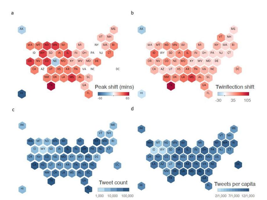
impact on human cognition is harmful in the workplace, and poses a pronounced and              15

distinct threat to public safety when operating a vehicle [7–10]. Short sleep is linked to     16

increased risk of serious health conditions, including heart disease, obesity, diabetes,       17

arthritis, depression, strokes, hypertension, and cancer [2, 11, 12], and a recent study       18

found that disrupted sleep is also associated with DNA damage [13]. The link between           19

sleep loss and cancer is so strong that the World Health Organization has classified           20

night shift work as “probably carcinogenic to humans” [14]. Socio-economic status is           21

positively correlated with quality of sleep [15–18]. Due to such detrimental effects, and      22

high prevalence among the population, insufficient sleep accounts for between $280 and         23

over $400 billion lost in the United States every year [19].                                   24

    Accurately measuring short sleep in a large population is difficult, and there is often    25

a trade-off between accuracy and the size of the study. Polysomnography—considered             26

the most accurate way to measure sleep—can only measure an individual’s sleep                  27

patterns in a controlled laboratory setting [20, 21]. Large studies have relied on             28

participants recording their own sleep, but suffer from reporting bias [2, 22, 23].            29

    Wearable technology can measure short sleep at the population scale, and has the           30

potential to measure short sleep accurately enough to study its association with adverse       31

health risks [4, 20, 24]. One recent large sleep study enrolled 31,000 participants and        32

used sleep data from wearable devices along with participant’s interactions with a web         33

based search engine to compare sleep loss and performance [4]. The authors [4] showed          34

that measurements of cognitive performance (including keystroke and click latency) vary        35

over time, follow a circadian rhythm, and are related to the duration of participant’s         36

sleep, results that closely mirrored those from laboratory settings and validated their        37

methodology.                                                                                   38

    While promising in the long run, present studies that use wearable devices have            39

limitations. To infer from wearables that individuals are sleeping, data must first go         40

through a pipeline of preprocessing, feature extraction and classification. The pipeline       41

for processing sleep data is typically proprietary and dependent on the specific wearable      42

used, and changes to how data is processed can impact results [25]. Moreover,                  43

validation studies have yet to explore the effectiveness of these devices across genders,      44

ages, culture, and health [25].                                                                45

    Social media may be an alternative way to measure sleep disturbances in a large            46

population, for example by studying the link between screen time and sleep [26, 27].           47

Researchers have found that Tweeting behavior can reveal ”sleep-wake” behavior for             48

individuals as well as cities [28, 29]. In particular, the correlation between sustained low   49

activity on Twitter and sleep time as measured by conventional surveys has been                50

validated against data collected from the CDC on sleep deprivation [26]. The                   51

relationship between time of onset of Twitter activity and wake time has been used to          52

explore and demonstrate social jetlag - the discrepancy between weekend and weekday            53

sleep behavior [26, 30]. Other work has shown evidence of an increase in a user’s smart        54

phone screen time as being associated with an increase in short sleep [27]. Other mental       55

and physical characteristics have been measured from sociotechnical systems. Several           56

instruments developed by members of our research group including the                           57

Hedonometer [31], which measures population sentiment through tweets, and the                  58

Lexicocalorimeter [32], which measures caloric balance at the state level, have                59

demonstrated an ability to infer population-scale health metrics from Twitter data.            60

Circadian rhythms in mood and cognitive processes have also been inferred from tweets          61

[33, 34]. Twitter data has also been used to identify users who experience sleep               62

deprivation and study the ways their social media interactions differ from others [35].        63

    In urban, industrialized societies where social timing is synced to clock time,            64

Daylight Savings- a biannual sudden upset to clock time- creates behavioral stability          65

across seasons [36, 37]. The onset of DST, Spring Forward, is associated with a one hour       66

                                                                                       2/19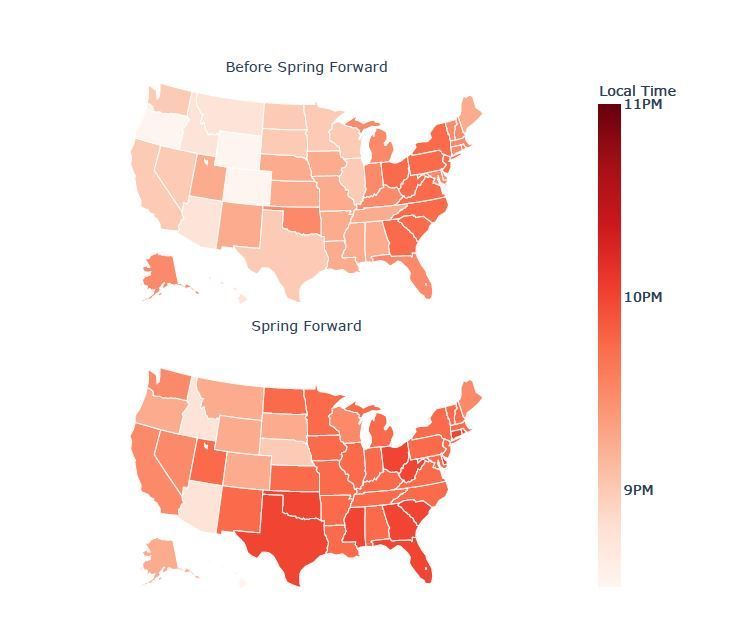
sleep disruption due to the disconnect between the ”human clock” and the mechanical            67

clock [38]. Past work has used Daylight Savings as a natural experiment to show that a         68

one hour collective sleep loss event has large and quantifiable effects on health, safety,     69

and the economy [39–42], with two striking findings being a one day increase in heart          70

attacks by 24% and a loss of $31 billion on the NYSE, AMEX, and NASDAQ exchanges               71

in the United States [39, 43].                                                                 72

    We hypothesize here that sleep loss is measurable in behavioral patterns on Twitter,       73

and changes in population-scale sleep patterns due to Spring Forward can be observed           74

through changes in these behavioral patterns. In what follows we first outline our             75

methodology for estimating sleep loss from tweets, describing the data and study design.       76

Then, we visualize and describe the results before concluding with a discussion of             77

limitation and implications.                                                                   78

Materials and methods                                                                          79

Data                                                                                           80

We collected a 10% random sample of all public tweets—offered by Twitter’s Decahose            81

API—for Sundays and Mondays in the four weeks leading up to, the week of, and the              82

four weeks following Spring Forward events during the years 2011-2014. Spring Forward          83

is defined as the instantaneous clock adjustment from 2 a.m. to 3 a.m. on the second           84

Sunday of March each year. We included tweets in the study if the user who created the         85

tweet reported living in the U.S. in their bio, or if the tweet was geo-tagged to a GPS        86

coordinate within the U.S. [44]. With these conditions, we ended up selecting                  87

approximately 7% of the messages in the Decahose random sample for analysis [45].              88

The sample was composed of 13.1 million tweets.                                                89

    Twitter provided the time-zone from which each message was posted during the               90

period from 2011 to 2014 (for privacy purposes, Twitter discontinued publication of            91

time zone information in 2015). We used the time-zone to determine the local time of           92

posting for each tweet. Tweets for which the time-zone was incompatible with the               93

assigned location were discarded. We binned tweets by 15 minute increments according           94

to the local time of day they were posted.                                                     95

Experimental setup                                                                             96

To estimate behavioral change associated with Daylight Savings, we partitioned tweets          97

 into various groups, primarily a “Before Spring Forward” (BSF) group and a “Spring            98

 Forward” (SF) group. To establish a convenient ‘control’ pattern of behavior, all tweets      99

 posted on any of the four Sundays before the Spring Forward event were classified as         100

“Before Spring Forward” tweets. We classified the ‘experimental’ set of tweets posted on      101

 the Sunday coincident with the Spring Forward event as “Spring Forward”. The above           102

 classification created, for every year, a 4:1 matching of before to week of Spring Forward   103

 activity. We analyzed tweets posted 1-4 weeks following Spring Forward separately to         104

 quantify relaxation to the original behavior.                                                105

Analysis                                                                                      106

We binned tweets by time in 15 minute intervals starting at the top of the hour, and          107

normalized their frequencies by dividing by the total number of tweets posted on the          108

corresponding day. In this way, we establish a discrete description of the posting volume     109

over the course of a typical 24-hour period.                                                  110

                                                                                      3/19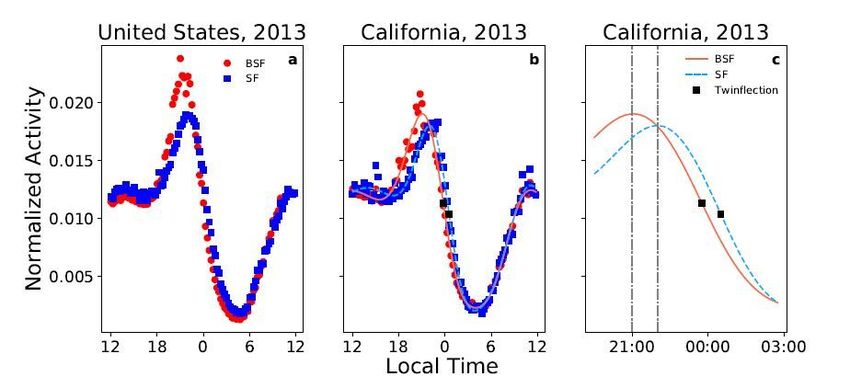
We averaged the Before Spring Forward tweets over the four Sundays, and the four
years as follows:
                                           2014   4
                                        −1
                                           X X       CY S (k)
                     TBSF (k) = (4 × 4)                       ,
                                                      CY S
                                                      Y =2011 S=1

where CY S (k) is the number of tweets in the k 15 minute interval of the S th Sunday
                                                         th
                                                                                              111

of year Y , CY S is the total number of tweets posted on that Sunday and year, and            112

TBSF (k) is the average fraction of tweets posted in the k th 15 minute interval of a         113

Sunday prior to Spring Forward,                                                               114

    We also normalized the Spring Forward tweets against daily activity:
                                                       2014
                                                 −1
                                                       X        CY (k)
                                 TSF (k) = (4)                         .
                                                                 CY
                                                      Y =2011

    These averages enabled us to aggregate more data, building a more reliable pattern
of daily activity, and decrease the susceptibility to daily variation. To reduce noise that
could depend on our choice of bin size and spatial scale, we smoothed normalized tweet
activity using Gaussian Process Regression (GPR) [46, 47]. We fit a GPR with a squared
exponential kernel and characteristic length scale of 150 minutes (a total of 10 bins of
size 15-minutes) to normalized tweets. We chose a characteristic length of 150 minutes
for consistency with previous work [26]. Tikhonov regularization with an α penalty
tuned manually to 0.1 was included when finding weights ωk to prevent overfitting [47].
GPR yielded a smooth behavioral curve, B(t), of the functional form:
                                 96
                                           "                 2 #
                                 X             1      t    tk
                         B(t) =     ωk exp − k           ,         ,
                                               2     150 150
                                   k=1

where ωk is a weight determined by the regression process, k is the squared-exponential       115

kernel (commonly called a radial basis), t is the time in minutes since midnight (00:00),     116

and tk is the k th 15 minute interval of the day, i.e. t5 corresponds to 75 minutes past      117

midnight, or 1:15 a.m. The sum to 96 refers to the number of 15 minute intervals in a         118

single 24 hour period.                                                                        119

    We generated behavioral curves B(t) for the BSF and SF groups by state, and for
the U.S. in aggregate. To estimate behavioral change induced by a Spring Forward
event, we calculate two quantities from the behavioral curves: (i) the time of peak
activity and (ii) the time of the inflection point between the peak and trough. The
inflection point is referred to as a ‘twinflection’ point, and represents a point of
diminishing losses in Twitter activity for the night. Peak shift is defined as:
                         arg max {BSF (t)} − arg max {BBSF (t)}
                             t                            t

and twinflection shift is defined as:
                                   ′                   ′
                         arg min {BSF (t)} − arg min {BBSF (t)},
                           t∈N                          t∈N

where N = {t : arg maxt B(t) < t < arg mint B(t)}. We were able to reliably measure           120

peak activity and twinflection because behavioral curves exhibited a consistent diurnal       121

wave structure: a rise in the evening corresponding to peak Twitter posting activity,         122

followed by a trough during typical sleeping hours, and a plateau throughout the day.         123

Contraction of the trough associated with sleeping hours is considered to be reflective of    124

lost sleep opportunity, and may indicate sleep loss itself.                                   125

    We measured the loss of sleep opportunity by calculating the peak and twinflection        126

times for the four weeks Before Spring Forward and the week of Spring Forward itself.         127

We then characterize differences between the BSF and SF measures for each state, and          128

for the total U.S., as a proxy for sleep loss.                                                129

                                                                                     4/19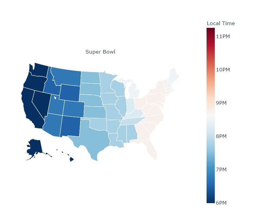
Results                                                                                                   130

Our overall finding is that peak Twitter activity occurs 15-30 minutes later on the                       131

Sunday evening immediately following Spring Forward for most states, with this shift                      132

varying among states. By Monday morning, activity is back to normal, suggesting that                      133

the window of sleep opportunity is visibly compressed in Twitter behavior.                                134

   In Fig 1, we plot B(t) for the subset of posts containing the words ‘breakfast’, ‘lunch’,              135

and ‘dinner’ for the period beginning 6 a.m. on Sunday and ending 9 p.m. on Monday,                       136

both before (solid) and after (dashed) Spring Forward events. These curves were                           137

constructed for states observing Eastern Time (top row) and Pacific Time (bottom row).                    138

These regions were chosen as they are the zones with the greatest spatial difference                      139

among zones with significant data density. Observing a shift in behavior for each assures                 140

us that these shifts are not limited to a particular geographic region of the country.                    141

                                           breakfast

                                                                                         Eastern
                         0.02                          dinner
   Normalized Activity

                                               lunch
                         0.01
                         0.00

                                                                                         Pacific
                         0.02
                         0.01
                         0.00
                              6       12          18        0         6   12   18
                             Sunday                      Local Time             Monday
Fig 1. Diurnal collective attention to meals quantified, by normalized usage
of the words ‘breakfast’, ‘lunch’, and ‘dinner’ for states observing Eastern
Time (top) and Pacific Time (bottom), for the weeks before (solid), and of
(dashed) Spring Forward. The x-axis represents the interval between 6 a.m. Sunday
and 9 p.m. Monday local time. Counts for tweets containing each individual word were
tallied in 15 minute increments, normalized by the total number of tweets mentioning
that word, and smoothed using Gaussian Process Regression. Each day has a clear
pattern for frequency of meal name appearance in tweets, with the peak for breakfast,
lunch, and dinner occurring in the respective order of the meals themselves. For each of
the meals, we observe a slight forward shift in the peak following Spring Forward,
suggesting that meals are taking place later than usual on the corresponding Sunday.
By Monday, the peak for each meal name appears to be aligned with the week before,
with the exception of ’dinner’ on the west coast, which is still a bit later.

   Meal-related language reveals a daily pattern of behavior in which peak volume                         142

occurs around the time that meal typically takes place. On an average Sunday,                             143

breakfast is most mentioned at 10:30 a.m., lunch at 1:15 p.m., and dinner at 6:45 p.m.                    144

in Eastern Time Zone states (see Fig 1). On the average Monday, breakfast mentions                        145

peak at 10:45 a.m., lunch peaks at 1:30 p.m., and dinner at 7:15 p.m. Breakfast and                       146

Lunch are mentioned more often on Sunday than on Monday.                                                  147

   There is essentially no discussion of meals during the period from 2 a.m.-6 a.m.                       148

These plots also exhibit a small forward shift in time following Spring Forward,                          149

suggesting that each meal was tweeted about, and probably eaten, later in the day on                      150

Sunday. The effect is greater on the East Coast, and disappears on both coasts by                         151

Monday.                                                                                                   152

                                                                                                   5/19
Broadening from messages mentioning specific meals to all messages, daily activity 153
plots of BBSF and BSF reveal a regular diurnal pattern of behavior that is consistently 154
shifted forward in time the evening following Spring Forward events. Fig 2 shows this 155
shift for the year 2013, but the results were similar for other years. 156
United States, 2013 California, 2013 California, 2013
BSF a b BSF c
SF SF
Twinflection
0.020
Normalized Activity
0.015
0.010
0.005
12 18 0 6 12 12 18 0 6 12 21:00 00:00 03:00
Local Time
Fig 2. Twitter activity behavioral curves B(t). (a) Normalized count of tweets
posted from a location within the United States between 12 p.m. Sunday and 12 p.m.
Monday before (red) and the week of (blue) the 2013 Spring Forward Event. The time
recorded for the tweet is that local to the author. Though the pattern of behavior is
preserved following Daylight Savings, peak activity is translated forward in time. (b)
The same plot, with location of tweet origin restricted to the state of California.
California is the state for which we have the most data, and therefore the most
representative behavior profile after smoothing with Gaussian Process Regression (lines).
We note that Fig 5 shows behavioral curves for all states. (c) The smoothed behavioral
pattern for California during the hours of 9 p.m. to 3 a.m. Pacific Time. Activity peaks
are denoted by vertical dashed lines, and twinflection points are marked by squares. To
estimate the behavioral shift in time, we compute the distance along the temporal axis
between these pairs of lines/points. California’s BSF peak is one hour earlier than the
SF peak.
Panel (a) suggests overall activity across the U.S. peaks around 9 p.m. on Sundays 157
before Spring Forward (red circles), and experiences a minimum around 5am. The peak 158
shifts approximately 45 minutes later on the Sunday of Spring Forward (blue squares) 159
before synchronizing again by early morning Monday. In panel (b) California is used as 160
an illustrative example of these patterns existing at the state level, and the smooth 161
behavioral pattern constructed using Gaussian Process Regression. The pattern is 162
similar to that observed for the entire country, with the exception of a slightly reduced 163
amplitude. Twinflection points are illustrated by black squares in panels (b) and (c). 164
Fig 2 demonstrates evidence that there is a shift in the peak time spent interacting 165
with Twitter on Sunday evening following Spring Forward, relative to prior Sundays. 166
Given the absence of a corresponding delay in interaction Monday morning, we infer an 167
decrease in sleep opportunity experienced on Sunday night. 168
To explore the spatial distribution of the behavioral changes induced by Spring 169
Forward, in Fig. 3 we map the time of peak Twitter activity on Sunday night for each 170
state before (top) and the week of (bottom) Spring Forward, averaged across the years 171
2011-2014. On the Sundays leading up to Spring Forward (top), peak twitter activity 172
occurs near either 10 p.m. for states on the East Coast, or 9:15 p.m., for most of the 173
other states. After Spring Forward, nearly all states exhibit peak activity later in the 174
6/19night. 175
Before Spring Forward
Local Time
11PM
10PM
Spring Forward
9PM
Fig 3. Time of peak Twitter activity on Sunday night for each state before
(top) and after (bottom) Spring Forward for the four events observed
between 2011 and 2014. Before Spring Forward, the time of peak activity occurs
around 10 p.m. most states in the Eastern Time Zone, and around 9:15- 9:30 p.m. for
most of the other states. After Spring Forward, peak Twitter activity occurs between 0
and 60 minutes later for each state, with the exception of Alaska, Nebraska, and Hawaii
for which the peak occured earlier. Texas has the latest peak at 10:15 p.m. local time, a
shift of 60 minutes forward compared with prior Sundays. We note again that the BSF
estimates are based on the aggregation of four Sundays prior to Spring Forward, while
the ASF estimates are based on the Sunday coincident with Spring Forward, and are
therefore estimated using roughly 1/4 the data. [48]
Looking at Texas as an individual example, before Spring Forward we see peak 176
activity around 9:15 p.m. local time, and after Spring Forward it occurs at 10:15 p.m. 177
local time. While Texas is one of the latest peaks observed on the evening following 178
Spring Forward, several other states are up late including Oklahoma, Georgia, and 179
Mississippi each peaking around 10:15 p.m as well. 180
In the Supplemental Information, we show maps estimating the time of peak activity 181
for each of the individual 9 weeks centered on Spring Forward (see Supplemenatry Fig 182
S1 online). There is some week-to-week variation, most notably in the second week prior 183
to Spring Forward, which was the night of the Academy Awards for three of the four 184
years. By four weeks after Spring Forward, the peak activity map has relaxed to 185
7/19roughly the same pattern as BSF. 186
The magnitude of the forward shift in behavior illustrated in Fig 3 is considered a 187
proxy for the loss of sleep opportunity on the Sunday night following Spring Forward. 188
We used two distinct methods to estimate this magnitude, namely the peak shift and 189
the twinflection shift. A comparison of the spatial estimates made using each method 190
are shown in Fig 4. 191
Panel (a) illustrates the average shift in peak activity observed for 2011-2014 by 192
computing the difference between the pair of maps in Fig 3 (bottom minus top). There 193
is clear spatial variation in the shift in time on the night of Spring Forward, while most 194
states exhibit a positive forward shift some exhibit none, and Alaska, Hawaii, and 195
Nebraska show a negative shift. The peak in Twitter behavior for the east and west 196
coasts occurred 0-30 minutes later Sunday night, while it occurred 30-60 minutes later 197
for the central U.S. (Fig 4 panel a). 198
Fig 4 panel (b) estimates the change using twinflection, namely the change in 199
concavity of the behavior activity curve from down to up. Every state except Hawaii, 200
Alaska, and Wyoming exhibits a shift forward in time, and with similar spatial 201
regularity. When measured with twinflection shift, Texas and Mississippi are seen to 202
have the greatest temporal shift following Spring Forward. Texans were tweeting 105 203
minutes later than usual following a Spring Forward event. Most of the east and west 204
coast states were measured as tweeting 15 to 30 minutes later (Fig 4 panel b). Both 205
measures agreed on a positive shift for the country as a whole. However, the two 206
measures yielded different results for the magnitude of these shifts, with twinflection 207
shift generally estimating a more positive shift. 208
Fig 4 panels (c) and (d) illustrate the amount of data contributing to calculations for 209
the behavioral curves, and the density of this data with respect to each state’s 210
population. Idaho, Alaska, Hawaii, Montana, Wyoming, North Dakota, South Dakota, 211
and Vermont were the states offering the smallest amount of data, and subsequently 212
have the highest potential for a poor behavioral curve model fit. Wyoming was unique 213
in that in 2013 for the 24 hour observation window on the week of spring forward there 214
were no tweets meeting inclusion requirements, making conclusions about this state 215
particularly tenuous. 216
Though the amount of data available for California and Texas is much greater than 217
the other states, when considering their large population size we find their twitter 218
activity per capita to be similar to most other states. Based on our estimate of tweets 219
per capita, we expect behavioral curves for most states to be more or less equally 220
representative of their tweeting populations. 221
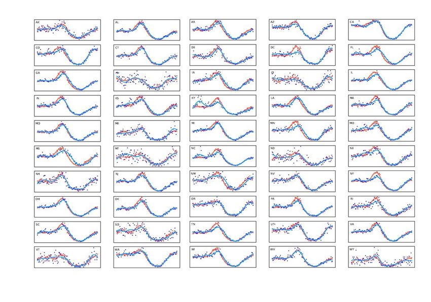
Looking at the diurnal cycle of Twitter activity for each individual state, we see 222
remarkable consistency. Fig. 5 shows the 24 hour period spanning noon Sunday to noon 223
Monday local time for the year 2012. Plots for the other 3 years exhibit similar 224
behavior. Before Spring Forward (red), most states show a peak between 9:15 and 10:00 225
p.m., local time. After Spring Forward (blue), nearly all states have a peak after 9:30 226
p.m. While states differ slightly in the time of peak, and magnitude of shift in the peak, 227
most exhibit a clear positive shift (see Supplementary Fig. S3 online). By Monday 228
morning, nearly all curves have re-aligned. We also consistently observe higher peaks for 229
the BSF curves which we believe to be driven by televised events such as the Oscars. 230
The Sunday of Spring Forward does not have a regularly scheduled popular television 231
event, and as a result the SF curves have lower amplitude. 232
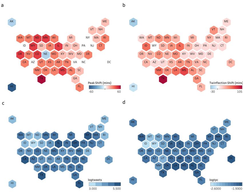
8/19Peak shift (mins) Twinflection shift
-30 35 105
Tweet count Tweets per capita
1,000 10,000 100,000 2/1,000 7/1,000 12/1,000
Fig 4. The magnitude of Twitter behavioral shift following a Spring
Forward event, averaged for the four years from 2011 to 2014. (a) Shift
measured using behavioral curve peaks, the difference between the pair of maps in
Figure 3 (bottom minus top). Texas is estimated to have experienced the greatest time
shift. The effect of Spring Forward is more pronounced in the South, and center of the
country. Alaska, Nebraska, and Hawaii have negative shifts. (b) The same map, but
with measurements calculated using twinflection shift instead. The states most affected
are Texas and Mississippi, where the shift was 105 and 75 minutes respectively. Hawaii
and Alaska are estimated to have negative shifts (15, and 30 minutes respectively).
Twinflection shift produces similar spatial results to peak shift, with greater shift
estimates. (c) The number of tweets posted from each state in the period after Spring
Forward. California and Texas both contributed over 200,000 tweets, while Alaska,
Hawaii, Idaho, Wyoming, Montana, North Dakota, South Dakota, Wyoming, Delaware,
New Hampshire, Maine and Vermont each produced less than 10,000 tweets. (d) The
density of data used to establish the experimental pattern of behavior, as measured by
tweets per capita. This measurement reflects the ability of the data to capture the
behavior of the tweeting population of each state. While Idaho, Wyoming, Montana,
Utah and South Dakota have relatively little data compared to their populations, the
remaining states have similar data density, with somewhere between five and eleven
tweets per thousand residents, with the exception of the District of Columbia which has
35. Note: both panels (c) and (d) use logarithmically spaced colorbars
9/19AK AL AR AZ CA
CO CT DE DC FL
GA HI IA ID IL
IN KS KY LA MA
MD ME MI MN MO
MS MT NC ND NE
NH NJ NM NV NY
OH OK OR PA RI
SC SD TN UT VA
VT WA WI WV WY
Fig 5. Normalized Twitter activity between 12 p.m. Sunday and 12 p.m. Monday prior to and following the 2012 Spring Forward
event for each state. Red indicates an aggregation of data from the specified period over four weeks before the Spring Forward Event. Blue indicates data
from the single 24 hour period after Spring Forward has occurred. Dots are indicative of ‘raw’ data, while the corresponding curves demonstrates Gaussian
smoothing. Texas exhibits the largest change following Spring Forward. Curves for nearly all states have aligned by Monday morning. The BSF peaks are
slightly higher than the SF peaks in some states, largely due to televised events Before Spring Forward such as the Oscars. The Sunday of Spring Forward does
not have a regularly scheduled popular television event, and as a result the SF curves have lower amplitude.Both the peak and twinflection demonstrate that it is possible to observe a 233
measurable decrease in the amount of sleep opportunity people in the United States 234
receive on average due to Spring Forward. They also both demonstrate uneven 235
geographic distribution of the effect of Spring Forward, and therefore the ability to 236
determine geographic disparity in sleep loss. 237
We also discovered that the Super Bowl occurred exactly 5 weeks prior to Spring 238
Forward in each of the years studied. This annual event watched by over 100 million 239
individuals in the U.S. caused peak Twitter activity to synchronize at roughly the same 240
time nationally, around 9 p.m. Eastern, during the second half of the football game. 241
The map in Fig 6 shows the time of peak activity for each state on Super Bowl Sunday, 242
averaged over the years 2011 to 2014. The colormap is the same as the scale used for 3, 243
with the additional cooler range brought in capture the time of peak relative to the 244
usual times. 245
The map bears a remarkable resemblance to the timezone map, demonstrating a 246
synchronization of collective attention across the country. Data from Super Bowl 247
Sunday was not included in the Before Spring Forward data, as it does not accurately 248
reflect the spatial distribution of typical posting behavior on a Sunday evening. 249
Discussion 250
Technically speaking, Spring Forward occurs very early Sunday morning, and the 251
instantaneous clock adjustment from 2 a.m. to 3 a.m. is witnessed by very few waking 252
individuals. In addition, we speculate that the majority of individuals do not set an 253
alarm clock for Sunday morning. As a result, we expect that the hour lost to Spring 254
Forward will be felt by our bodies most meaningfully on Monday morning. Indeed, we 255
are likely to experience the Monday morning alarm as occurring an hour early, as 256
Spring Forward shortens the time typically reserved for sleep opportunity Sunday night 257
by one hour. 258
Considering the correlation between screen time and lack of sleep, the Sunday 259
evening shift, and the corresponding Monday morning re-synchronization, we observe 260
evidence that sleep opportunity is lost in some states on the evening of Spring Forward. 261
By estimating the magnitude and spatial distribution of the shift in Twitter behavioral 262
curves, we have approximated a lower bound on sleep loss at the state level. 263
Our pair of measurement methodologies have a Pearson correlation coefficient of 264
0.575, and a Spearman correlation coefficient of 0.467 (See Supplementary Fig S3 online 265
While they produced slightly different estimates of the magnitude of temporal shift in 266
behavior, the resulting geographic profiles of sleep loss were similar. Both suggest that 267
states along the coast are least affected by Spring Forward, while Texas and the states 268
surrounding it to the North and East are the most affected. 269
Peak shift suggests the temporal shift in behavior due to Spring Forward generally 270
less than the actual clock shift (1 hour). California, the state for which we have the 271
most data and therefore the most representative behavior profile after smoothing, was 272
found to have a peak shift of 30 minutes. 273
Considering the clock adjustment of exactly one hour, both measurements are 274
plausibly directly representative of sleep lost, however the differing magnitudes of the 275
measurements indicate that future work should clarify the relationship between these 276
measurements and actual shifts. Twinflection measured similar shifts for most states, 277
but for a few estimated larger effects. While California was measured as having the 278
same 30 minute shift, Texas, the state for which we have the second most data, was 279
estimated by twinflection to be delayed by an additional 45 minutes. 280
Twinflection measured a small forward shift for the state of Arizona, which does not 281
observe DST. This could indicate that the twinflection method overestimates the 282
11/19Local Time
11PM
Super Bowl
10PM
9PM
8PM
7PM
6PM
Fig 6. Peak activity time (local) for Super Bowl Sunday, 5 weeks prior to
Spring Forward, averaged over the years 2011 to 2014. Activity exhibits a
clear resemblance to the U.S. timezone map, with a peak near 9 p.m. Eastern Time just
following the halftime performance. The data suggests a national collective
synchronization in attention. Green Bay Packers d. Pittsburgh Steelers (2011), New
York Giants d. New England Patriots (2012), Baltimore Ravens d. San Francisco 49ers
(2013), and Seattle Seahawks d. Denver Broncos (2014). Performers included The Black
Eyed Peas, Usher, and Slash (2011), Madonna, LMFAO, Cirque du Soleil, Nicki Minaj,
M.I.A., and Cee Lo Green (2012), Beyoncé, Destiny’s Child (2013), and Bruno Mars,
Red Hot Chili Peppers (2014). We note that the colormap here the same as the scale
used for 3, with blue colors included to reflect the relatively early times of the peaks
relative to the other weeks.
behavioral shift. It is also possible that a shift in behavior could occur for residents of 283
Arizona, as a result of their connections to those in neighboring states, and in their 284
former timezone. In example, some residents likely work in bordering states, and are 285
forced to observe DST, and some will likely engage in more online activity and 286
discussion when their peers are present- those peers being initially established by a 287
shared time of activity. This we believe to be an important distinction between Arizona 288
and Hawaii, which also does not observe DST. 289
Hawaii is measured to have gained sleep opportunity by both accounts. Lacking the 290
observation of DST, neighboring states, and other states in the same timezone, it is 291
plausible that behavior in Hawaii would be unlike any other state, and be more 292
12/19independent of behaviors in other states. However, Hawaii’s results should be 293
considered tentative at best, given the sparsity of data available. This sparsity of data 294
and relative independence from other states is shared with Alaska, the other state with 295
a measured sleep opportunity gain by both measures. Caution should likewise be 296
extended to measurements ascribed to South Dakota, North Dakota, Wyoming, Idaho, 297
Montana, Vermont, New Hampshire, Rhode Island, Delaware, and Maine. These states 298
have smaller populations, less population density, and lower volume of tweets. As a 299
result, the behavioral curves associated with these states are less reliable. 300
Discrepancies in available data were determined to be largely accounted for by 301
differences in population. Thus, we expect results for each state (exclusive of those 302
mentioned earlier) to be comparably reliable in their representation of sleep loss for the 303
state as a whole. 304
Incremental future work in this area could investigate state specific sleep loss related 305
to Spring Forward events, which would allow further clarification of the relationship 306
between the magnitude of behavioral shifts on Twitter and population sleep loss. Other 307
directions might include looking at other sleep opportunity interruption events such as 308
the end of Daylight Savings in November, where we are ostensibly given an additional 309
hour of sleep opportunity. Our findings suggest that the sleep behavior associated with 310
other annual events including New Year’s Eve and Thanksgiving ought to be visible 311
through tweets. This and other works would also benefit from exploration of the 312
relationship between measurements of sleep opportunity as given by social media 313
activity and actual sleep duration. More ambitiously, proxy data such as this could be 314
verified by matching wearable measurements of sleep (e.g. Fitbit) with social media 315
accounts. 316
Our study suffers from several limitations associated with our data source, we 317
describe a few such examples here. The geographic location users provide in their 318
Twitter bio is static and unlikely to be updated when traveling. As a result, user 319
locations (time zone, state) inferred from this field will not always reflect their precise 320
location. The GPS tagged messages included in our analysis will not suffer from this 321
same uncertainty. Furthermore, the tweeting population of each state is likely to have 322
complicated biases with respect to their representation of the general population [49]. 323
Our dataset likely contains automated activity. Indeed, an entire ecology of 324
algorithmic tweets evolved during the period in which we collected data for this study. 325
However, we expect the majority of this activity to be scheduled using software that 326
updates local time automatically in response to Daylight Savings. As such, this ‘bot’ 327
type activity should largely serve to reduce our estimate of the time shift exhibited by 328
humans. 329
As we showed for the Super Bowl, live televised events (e.g. sports, awards shows) 330
have the potential to be a forcing mechanism to synchronize our collective attention 331
throughout the week, and especially on Sunday evenings. Indeed, many individuals take 332
to Twitter as a second screen during such events to interact with other viewers. In 333
addition, streaming services such as Netflix and HBO often release new episodes of 334
popular shows on Sunday night to align with peak consumption opportunity. These 335
cultural attractions exert a temporal organizing influence on our leisure behavior, and 336
the Spring Forward disturbance translates this synchronization forward in time. 337
It is worth noting that early March is a rather dull time of year for popular 338
professional sports in the United States. While the National Basketball Association and 339
National Hockey League are finishing up their regular seasons, the National Football 340
League is in its off-season and Major League Baseball beginning pre-season exercises. 341
Arguably the most engaging live-televised sporting contests taking place in early March 342
are the NCAA College Basketball Conference Championship games, with March 343
Madness happening weeks after Spring Forward. 344
13/19In 2014, the Academy Awards were hosted by Ellen DeGeneres on Sunday March 2. 345
Her famous selfie tweet containing many famous actors was posted that evening, a 346
message which held the record for most retweeted status update for several years [50]. 347
The event happened the week before Spring Forward, and led to anomalous behavior 348
compared with all other Sundays we looked at. 349
Since Spring Forward only occurs once per year, the specific language of the tweets 350
is highly dependent on events occurring on that specific day. The variability in daily 351
events and susceptibility of affect to these daily events makes study of the actual 352
language in the tweets unreliable. 353
Finally, Twitter (and other social media companies) have access to much higher 354
fidelity information regarding user activity than we have analyzed here. We are not able 355
to analyze consumption activity on the site, e.g. when individual messages are 356
interacted with via views, likes, or clicks. These forms of interaction with the Twitter 357
ecosystem are likely to occur chronologically following the final posting of a message in 358
the evening, and prior to the initial posting of a message in the morning. As a result, 359
we expect our estimate of the sleep opportunity lost due to Spring Forward to be a 360
lower bound. 361
Conclusion 362
Privacy preserving passive measurement of daily behavior has tremendous potential to 363
transform population-scale human activity into public health insight. The present study 364
demonstrates a proof-of-concept along the path to a far more ambitious goal: 365
construction of an ‘Insomniometer’ capable of real-time estimation of large-scale sleep 366
duration and quality. Which cities in the U.S. slept well last night? Which states are 367
increasingly suffering from insomnia? Answers to questions like these are not available 368
today, but could lead to better public health surveillance in the near future. For 369
example, communities exhibiting disrupted sleep in a collective pattern may be in the 370
early stages of the outbreak of the flu or some other virus. Current methodologies for 371
answering these questions are not scalable, but social media, mobile devices, and 372
wearable fitness trackers offer a new opportunity for improved monitoring of public 373
health. 374
Acknowledgements 375
KL, TA, PSD, and CMD thank MassMutual for contributing funding in support of this 376
research. The authors thank Adam Fox, Marc Maier, Jane Adams, David Dewhurst, 377
Lewis Mitchell, and Henry Mitchell for helpful conversations. 378
Author Contributions 379
Research question was formulated by KL, CMD, PSD, and JL. Data manipulations were 380
performed by KL and MA. Figures were generated by KL.Data analysis was performed 381
by KL, and CMD. Writing was done by KL, TM, and CMD. Revisions were made by 382
KL, TA, TM, CMD, PSD, and JL. 383
Competing Interests 384
The authors are unaware of any competing interests at this time. 385
14/19Data Availability 386
Message counts used to construct behavioral curves are available at the paper’s 387
associated GitLab repository: (to be built). We used Twitter’s gardenhose stream (10% 388
of all tweets); we do not share messages for privacy reasons, and our data products and 389
results are population-scale artifacts. Using samples of tweets from the same time 390
periods will generate similar results. 391
15/19References
1. Panel CC, Watson NF, Badr MS, Belenky G, Bliwise DL, Buxton OM, et al.
Joint consensus statement of the American Academy of Sleep Medicine and Sleep
Research Society on the recommended amount of sleep for a healthy adult:
Methodology and discussion. Sleep. 2015;38(8):1161–1183.
2. Short Sleep Duration Among US Adults; 2017.
3. Ford ES, Cunningham TJ, Croft JB. Trends in self-reported sleep duration
among US adults from 1985 to 2012. Sleep. 2015;38(5):829–832.
4. Althoff T, Horvitz E, White RW, Zeitzer J. Harnessing the Web for
Population-Scale Physiological Sensing: A Case Study of Sleep and Performance.
WWW ’17 Proceedings of the 26th International Conference on World Wide Web.
2017; p. 113–122.
5. Curcio G, Ferrara M, De Gennaro L. Sleep loss, learning capacity and academic
performance. Sleep Medicine Reviews. 2006;10(5):323–337.
6. Engle-Friedman M. The effects of sleep loss on capacity and effort. Sleep Science.
2014;7(4):213–224.
7. Rosekind MR, Gregory KB, Mallis MM, Brandt SL, Seal B, Lerner D. The cost
of poor sleep: Workplace productivity loss and associated costs. Journal of
Occupational and Environmental Medicine. 2010;52(1):91–98.
8. Dean B, Aguilar D, Shapiro C, Orr WC, Isserman JA, Calimlim B, et al.
Impaired health status, daily functioning, and work productivity in adults with
excessive sleepiness. Journal of Occupational and Environmental Medicine.
2010;52(2):144–149.
9. Owens J, Dingus T, Guo F, Fang Y, Perez M, McClafferty J, et al. Prevalence of
drowsy-driving crashes: Estimates from a large-scale naturalistic driving study.
AAA Foundation for Traffic Safety. 2018;.
10. Anderson C, Ftouni S, Ronda JM, Rajaratnam SM, Czeisler CA, Lockley SW.
Self-reported drowsiness and safety outcomes while driving after an extended
duration work shift in trainee physicians. Sleep. 2018;41(2):zsx195.
11. Medic G, Wille M, Hemels ME. Short-and long-term health consequences of sleep
disruption. Nature and Science of Sleep. 2017;9:151.
12. Nagai M, Hoshide S, Kario K. Sleep duration as a risk factor for cardiovascular
disease-a review of the recent literature. Current cardiology reviews.
2010;6(1):54–61.
13. Cheung V, Yuen V, Wong G, Choi S. The effect of sleep deprivation and
disruption on DNA damage and health of doctors. Anaesthesia.
2019;74(4):434–440.
14. Fox M. Shift work may cause cancer, world agency says. Reuters. 2007;.
15. Patel NP, Grandner MA, Xie D, Branas CC, Gooneratne N. “Sleep disparity” in
the population: Poor sleep quality is strongly associated with poverty and
ethnicity. BMC Public Health. 2010;10(1):475.
16/1916. Chattu VK, Chattu SK, Spence DW, Manzar MD, Burman D, Pandi-Perumal
SR. Do Disparities in Sleep Duration Among Racial and Ethnic Minorities
Contribute to Differences in Disease Prevalence? Journal of Racial and Ethnic
Health Disparities. 2019;6(6):1053–1061.
17. Ruiter ME, DeCoster J, Jacobs L, Lichstein KL. Normal sleep in
African-Americans and Caucasian-Americans: A meta-analysis. Sleep Medicine.
2011;12(3):209–214.
18. Curtis DS, Fuller-Rowell TE, El-Sheikh M, Carnethon MR, Ryff CD. Habitual
sleep as a contributor to racial differences in cardiometabolic risk. Proceedings of
the National Academy of Sciences. 2017;114(33):8889–8894.
19. Hafner M, Stepanek M, Taylor J, Troxel WM, Van Stolk C. Why sleep
matters—the economic costs of insufficient sleep: A cross-country comparative
analysis. Rand Health Quarterly. 2017;6(4).
20. Bianchi MT. Sleep devices: Wearables and nearables, informational and
interventional, consumer and clinical. Metabolism. 2018;84:99–108.
21. Douglas NJ, Thomas S, Jan MA. Clinical value of polysomnography. The Lancet.
1992;339(8789):347–350.
22. Harvey AG, Tang NK. (Mis) perception of sleep in insomnia: A puzzle and a
resolution. Psychological Bulletin. 2012;138(1):77.
23. Lauderdale DS, Knutson KL, Yan LL, Liu K, Rathouz PJ. Self-reported and
measured sleep duration: How similar are they? Epidemiology. 2008; p. 838–845.
24. Marino M, Li Y, Rueschman MN, Winkelman JW, Ellenbogen J, Solet JM, et al.
Measuring sleep: Accuracy, sensitivity, and specificity of wrist actigraphy
compared to polysomnography. Sleep. 2013;36(11):1747–1755.
25. Roomkham S, Lovell D, Cheung J, Perrin D. Promises and challenges in the use
of consumer-grade devices for sleep monitoring. IEEE Reviews in Biomedical
Engineering. 2018;11:53–67.
26. Leypunskiy E, Kıcıman E, Shah M, Walch OJ, Rzhetsky A, Dinner AR, et al.
Geographically resolved rhythms in Twitter use reveal social pressures on daily
activity patterns. Current Biology. 2018;28(23):3763–3775.
27. Christensen MA, Bettencourt L, Kaye L, Moturu ST, Nguyen KT, Olgin JE,
et al. Direct measurements of smartphone screen-time: Relationships with
demographics and sleep. PLOS ONE. 2016;11(11).
28. Rios M, Lin J. Visualizing the Pulse of World Cities on Twitter. Proceedings of
the Seventh International AAAI Conference on Weblogs and Social Media; p. 4.
29. Roenneberg T. Twitter as a means to study temporal behaviour. Current
Biology. 2017;27(17):R830–R832. doi:10.1016/j.cub.2017.08.005.
30. Scheffler T, Kyba CCM. Measuring Social Jetlag in Twitter Data. Proceedings of
the Tenth International AAAI Conference on Web and Social Media (ICWSM
2016); p. 4.
31. Dodds PS, Harris KD, Kloumann IM, Bliss CA, Danforth CM. Temporal
patterns of happiness and information in a global social network: Hedonometrics
and Twitter. PLOS ONE. 2011;6(12).
17/1932. Alajajian SE, Williams JR, Reagan AJ, Alajajian SC, Frank MR, Mitchell L,
et al. The Lexicocalorimeter: Gauging public health through caloric input and
output on social media. PLOS ONE. 2017;12(2).
33. Dzogang F, Lightman S, Cristianini N. Circadian mood variations in Twitter
content. Brain and Neuroscience Advances. 2017;1:2398212817744501.
doi:10.1177/2398212817744501.
34. Dzogang F, Lightman S, Cristianini N. Diurnal variations of psychometric
indicators in Twitter content. PLOS ONE. 2018;13(6):e0197002.
doi:10.1371/journal.pone.0197002.
35. McIver DJ, Hawkins JB, Chunara R, Chatterjee AK, Bhandari A, Fitzgerald TP,
et al. Characterizing sleep issues using Twitter. Journal of Medical Internet
Research. 2015;17(6):e140.
36. Martı́n-Olalla JM. the long term impact of Daylight Saving time regulations in
daily life at several circles of latitude. Scientific Reports. 2019;9(1):1–13.
37. Martı́n-Olalla JM. Scandinavian bed and rise times in the Age of Enlightenment
and in the 21st century show similarity, helped by Daylight Saving Time. Journal
of Sleep Research. 2019;doi:10.1111/jsr.12916.
38. Kantermann T, Juda M, Merrow M, Roenneberg T. The Human Circadian
Clock’s Seasonal Adjustment Is Disrupted by Daylight Saving Time. Current
Biology. 2007;17(22):1996–2000. doi:10.1016/j.cub.2007.10.025.
39. Sandhu A, Seth M, Gurm HS. Daylight Savings Time and myocardial infarction.
Open Heart. 2014;1(1):e000019.
40. Sipilä JO, Ruuskanen JO, Rautava P, Kytö V. Changes in ischemic stroke
occurrence following Daylight Saving Time transitions. Sleep Medicine.
2016;27:20–24.
41. Varughese J, Allen RP. Fatal accidents following changes in Daylight Savings
Time: The American experience. Sleep Medicine. 2001;2(1):31–36.
42. Martı́n-Olalla JM. Traffic accident increase attributed to Daylight Saving Time
doubled after Energy Policy Act. Current Biology. 2020;30(7):R298–R300.
doi:10.1016/j.cub.2020.03.007.
43. Kamstra MJ, Kramer LA, Levi MD. Losing sleep at the market: The Daylight
Saving anomaly. American Economic Review. 2000;90(4):1005–1011.
44. Gray TJ, Reagan AJ, Dodds PS, Danforth CM. English verb regularization in
books and tweets. PLOS ONE. 2018;13(12).
45. Twitter. Developer application program interface (API); 2020.
https://developer.twitter.com/en/docs/tweets/sample-
realtime/overview/decahose.
46. Rasmussen CE. Gaussian processes in machine learning. In: Summer School on
Machine Learning. Springer; 2003. p. 63–71.
47. Pedregosa F, Varoquaux G, Gramfort A, Michel V, Thirion B, Grisel O, et al.
Scikit-learn: Machine learning in Python. Journal of Machine Learning Research.
2011;12(Oct):2825–2830.
18/1948. Inc PT. Collaborative data science; 2015. Available from: https://plot.ly.
49. Wojcik S, Hughes A. Sizing up Twitter users; 2019.
50. DeGeneres E; March 2, 2014.
https://twitter.com/theellenshow/status/440322224407314432.
19/19Figures Figure 1 Diurnal collective attention to meals quanti ed, by normalized usage of the words breakf ′ , lunch', and `dinner' for states observing Eastern Time (top) and Paci c Time (bottom), for the weeks before (solid), and of (dashed) Spring Forward. The x-axis represents the interval between 6 a.m. Sunday and 9 p.m. Monday local time. Counts for tweets containing each individual word were tallied in 15 minute increments, normalized by the total number of tweets mentioning that word, and smoothed using Gaussian Process Regression. Each day has a clear pattern for frequency of meal name appearance in tweets, with the peak for breakfast, lunch, and dinner occurring in the respective order of the meals themselves. For each of the meals, we observe a slight forward shift in the peak following Spring Forward, suggesting that meals are taking place later than usual on the corresponding Sunday. By Monday, the peak for each meal name appears to be aligned with the week before, with the exception of 'dinner' on the west coast, which is still a bit later.
Figure 2

Twitter activity behavioral curves B(t). (a) Normalized count of tweets posted from a location within the
United States between 12 p.m. Sunday and 12 p.m. Monday before (red) and the week of (blue) the 2013
Spring Forward Event. The time recorded for the tweet is that local to the author. Though the pattern of
behavior is preserved following Daylight Savings, peak activity is translated forward in time. (b) The
same plot, with location of tweet origin restricted to the state of California. California is the state for
which we have the most data, and therefore the most representative behavior pro le after smoothing with
Gaussian Process Regression (lines). We note that Fig 5 shows behavioral curves for all states. (c) The
smoothed behavioral pattern for California during the hours of 9 p.m. to 3 a.m. Paci c Time. Activity
peaks are denoted by vertical dashed lines, and twin ection points are marked by squares. To estimate
the behavioral shift in time, we compute the distance along the temporal axis between these pairs of
lines/points. California's BSF peak is one hour earlier than the SF peak.
Figure 3

Time of peak Twitter activity on Sunday night for each state before (top) and after (bottom) Spring
Forward for the four events observed between 2011 and 2014. Before Spring Forward, the time of peak
activity occurs around 10 p.m. most states in the Eastern Time Zone, and around 9:15- 9:30 p.m. for most
of the other states. After Spring Forward, peak Twitter activity occurs between 0 and 60 minutes later for
each state, with the exception of Alaska, Nebraska, and Hawaii for which the peak occured earlier. Texas
has the latest peak at 10:15 p.m. local time, a shift of 60 minutes forward compared with prior Sundays.
We note again that the BSF estimates are based on the aggregation of four Sundays prior to Spring
Forward, while the ASF estimates are based on the Sunday coincident with Spring Forward, and are
therefore estimated using roughly 1/4 the data. [48] Note: The designations employed and the
presentation of the material on this map do not imply the expression of any opinion whatsoever on the
part of Research Square concerning the legal status of any country, territory, city or area or of its
authorities, or concerning the delimitation of its frontiers or boundaries. This map has been provided by
the authors.

Figure 4

The magnitude of Twitter behavioral shift following a Spring Forward event, averaged for the four years
from 2011 to 2014. (a) Shift measured using behavioral curve peaks, the difference between the pair of
maps in Figure 3 (bottom minus top). Texas is estimated to have experienced the greatest time shift. The
effect of Spring Forward is more pronounced in the South, and center of the country. Alaska, Nebraska,
and Hawaii have negative shifts. (b) The same map, but with measurements calculated using
twin ection shift instead. The states most affected are Texas and Mississippi, where the shift was 105
and 75 minutes respectively. Hawaii and Alaska are estimated to have negative shifts (15, and 30
minutes respectively). Twin ection shift produces similar spatial results to peak shift, with greater shift
estimates. (c) The number of tweets posted from each state in the period after Spring Forward. California
and Texas both contributed over 200,000 tweets, while Alaska, Hawaii, Idaho, Wyoming, Montana, North
Dakota, South Dakota, Wyoming, Delaware, New Hampshire, Maine and Vermont each produced less
than 10,000 tweets. (d) The density of data used to establish the experimental pattern of behavior, as
measured by tweets per capita. This measurement re ects the ability of the data to capture the behavior
of the tweeting population of each state. While Idaho, Wyoming, Montana, Utah and South Dakota have
relatively little data compared to their populations, the remaining states have similar data density, with
somewhere between ve and eleven tweets per thousand residents, with the exception of the District of
Columbia which has 35. Note: both panels (c) and (d) use logarithmically spaced colorbars Note: The
designations employed and the presentation of the material on this map do not imply the expression of
any opinion whatsoever on the part of Research Square concerning the legal status of any country,
territory, city or area or of its authorities, or concerning the delimitation of its frontiers or boundaries. This
map has been provided by the authors.

Figure 5

Normalized Twitter activity between 12 p.m. Sunday and 12 p.m. Monday prior to and following the 2012
Spring Forward event for each state. Red indicates an aggregation of data from the speci ed period over
four weeks before the Spring Forward Event. Blue indicates data from the single 24 hour period after
Spring Forward has occurred. Dots are indicative of `raw' data, while the corresponding curves
demonstrates Gaussian smoothing. Texas exhibits the largest change following Spring Forward. Curves
You can also read