Federal Reserve Bank of Minneapolis - Banking Without Deposit Insurance or Bank Panics: Lessons From a Model of the U.S. National Banking System ...
←
→
Page content transcription
If your browser does not render page correctly, please read the page content below
Federal Reserve Bank
of Minneapolis

Banking Without Deposit Insurance
or Bank Panics: Lessons From
a Model of the U.S. National
Banking System (p. 3)
V. V. Chari

Bank Failures, Financial Restrictions,
and Aggregate Fluctuations:
Canada and the United States,
1870-1913 (p. 20)
Stephen D. Williamson
Federal Reserve Bank of Minneapolis

Quarterly Review
Vol. 13, No. 3        ISSN 0271-5287

This publication primarily presents economic research aimed at improving
policymaking by the Federal Reserve System and other governmental
authorities.

Produced in the Research Department. Edited by John H. Boyd, Kathleen
S. Rolfe, and Inga Velde. Graphic design by Terri Gane, Public Affairs
Department.

Address questions to the Research Department, Federal Reserve Bank,
Minneapolis, Minnesota 55480 (telephone 612-340-2341).

Articles may be reprinted if the source is credited and the Research
Department is provided with copies of reprints.

 The views expressed herein are those of the authors and not
necessarily those of the Federal Reserve Bank of Minneapolis or
the Federal Reserve System.
Federal Reserve Bank of Minneapolis
     Quarterly Review Summer 1989

     Bank Failures, Financial Restrictions, and Aggregate Fluctuations:
     Canada and the United States, 1870-1913*

     Stephen D. Williamson t
     Associate Professor
     Department ol Economics
     University of Western Ontario

The belief that bank runs and failures contribute to        explanations for bank runs; insights into the role of
instability in aggregate economic activity is both long-    financial intermediaries in aggregate fluctuations; and
standing and widely held. Indeed, the Federal Reserve       implications for the effects of financial regulations.
Act of 1913 and the Banking Act of 1933 and of 1935             One branch of this financial intermediation litera-
were partly intended to correct what were thought to be     ture, stemming from the work of Diamond and Dybvig
inherent instabilities in the banking industry. Such leg-   (1983), focuses on deposit contracts, bank runs, and
islation, it was hoped, would reduce or eliminate these     bank failures. In the Diamond and Dybvig model, the
inherent instabilities and thereby reduce the magnitude     banking system has an inherent instability. Banks pro-
of fluctuations in all economic activity. This paper        vide a form of insurance through the withdrawal provi-
challenges the conventional wisdom about the histori-       sion in deposit contracts. But then banks are left open
cal causes of bank runs and failures and about the          to runs, during which the expectation of the failure of
relationship between these runs and failures and aggre-     an otherwise safe bank is self-fulfilling. (This branch of
gate activity. This challenge is based on a theoretical     the literature includes Postlewaite and Vives 1987,
approach that explicitly models financial intermedia-       Wallace 1988, and Williamson 1988.)
tion and monetary arrangements and on a comparative             Another branch of the financial intermediation
study of banking and aggregate fluctuations in the          literature—which includes work by Diamond (1984),
United States and Canada during the years 1870-1913.        Boyd and Prescott (1986), and Williamson (1986)—
   In a previous Quarterly Review article (Williamson       is concerned with financial intermediation in general
1987b), I reviewed some recent developments in the
theory of financial intermediation. This new financial           *This paper is adapted from an article, "Restrictions on Financial
intermediation literature is somewhat diverse, but the      Intermediaries and Implications for Aggregate Fluctuations: Canada and the
                                                            United States, 1870-1913," in the NBER Macroeconomics Annual 1989,
models generally follow the approach of specifying          © 1989 by The National Bureau of Economic Research and The Massachusetts
an economic environment in terms of primitives—             Institute of Technology. It is adapted here by permission of MIT Press. The
preferences, endowments, and technology—and then            author thanks David Backus for the use of a program for computing Hodrick-
                                                            Prescott filters, and Frank Lewis for assistance with historical sources. He also
analyzing how that environment generates financial          thanks Olivier Blanchard, Mark Gertler, David Laidler, Julio Rotemberg,
intermediation. Several things are gained from this type    Lawrence White, seminar participants at the Federal Reserve Bank of
of approach: a deeper understanding of the role of          Minneapolis, and conference participants at the National Bureau of Economic
                                                            Research for their helpful comments.
financial intermediaries as institutions that diversify,
                                                               fFormerly Economist, Research Department, Federal Reserve Bank of
transform assets, and process information; possible         Minneapolis.

20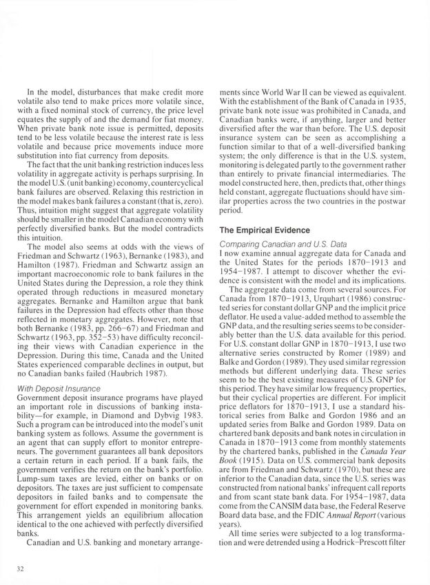
Stephen D. Williamson
  Bank Failures

(rather than banking in particular). It is also concern-      banking system with about 40 chartered banks. In
ed with the features of economic environments (mor-           contrast (in 1890), the United States had more than
al hazard, adverse selection, and monitoring and              8,000 banks, mostly unit banks. Numerous restrictions
evaluation costs) that can lead to intermediary struc-        on branching, along with other constraints absent in
tures. Models of this type have been integrated into          Canada, tended to keep U.S. banks small. Canadian
macroeconomic frameworks by Williamson (1987c),               banks were free to issue private circulating notes with
Bernanke and Gertler (1989), and Greenwood and                few restrictions on their backing, but all circulating
Williamson (1989) to study the implications of finan-         currency in the United States was effectively an obli-
cial intermediation for aggregate fluctuations. A gen-        gation of the U.S. government. In addition to these
eral conclusion of this work is that the financial interme-   differences in banking and monetary arrangements, the
diation sector tends to amplify fluctuations. Bernanke        countries had different records of bank runs and
and Gertler (1989) show how a redistribution of wealth        failures. Average bank depositor losses as a fraction of
from borrowers to lenders increases the agency costs          deposits were roughly 60 percent larger in the United
associated with lending, thereby causing a decrease in        States than in Canada. Also, cooperative behavior
the quantity of intermediation and in real output. Such       among Canadian banks acted to virtually preempt any
a wealth redistribution might be associated with debt         widespread banking panics, so that disruption from
deflations. Williamson (1987c) shows how some kinds           financial crises was considerably smaller in Canada. In
of aggregate technology shocks, which produce no              marked contrast, widespread bank runs and failures
fluctuations in an environment without the information        characterized U.S. history during the National Banking
costs that generate an intermediary structure, do cause       Era (1864-1913), as documented by Sprague (1910).
fluctuations when these costs are present. (See Gertler           The model presented here captures the important
1988 for a survey of other related work.)                     features of Canadian and U.S. monetary and banking
   This paper has two purposes. First, for those unfamil-     arrangements during 1870-1913. It is related to other
iar with the recent literature on financial intermediation,   models constructed by Williamson (1987c) and Green-
it shows how an explicit general equilibrium model            wood and Williamson (1989) in that it has costly state
with endogenous financial intermediation can illumi-          verification (Townsend 1979), which provides a dele-
nate some central issues in banking and macroeco-             gated monitoring role for financial intermediaries
nomics and can organize some historical experience            (Diamond 1984, Williamson 1986). When the model
and empirical evidence. Second, for those familiar with       includes a restriction on diversification by financial
the intermediation literature, this paper shows how a         intermediaries, interpreted here as a unit banking re-
model related to models of Williamson (1987c) and             striction, banks fail with positive probability. When
Greenwood and Williamson (1989) can be used to                they fail, banks experience something that can be inter-
study bank runs and failures. The model here has some         preted as a bank run. In contrast, banks not subject
novel implications for the role of financial regulations      to the unit banking restriction diversify perfectly and
and bank failures in aggregate fluctuations, and I find       never fail.
some (qualified) empirical support for its predictions.           When subjected to aggregate technological shocks,
   The approach I take is the following. First, I study a     the model yields patterns of comovement in the data
historical period when monetary and banking arrange-          that are qualitatively similar whether or not there is a
ments in two countries were strikingly different but          unit banking restriction or a constraint that banks
when other factors affecting aggregate fluctuations           cannot issue circulating notes. The price level, bank
were quite similar. Next, I construct a general equi-         liabilities, and output are mutually positively corre-
librium model with endogenous financial intermedia-           lated. Two important results are
tion. The model can incorporate the financial arrange-
ments of each country as special cases. Then I study the         •Under the unit banking restriction, bank failures
implications of the differences in banking and mone-              are high when output is low, but the unit banking
tary arrangements for aggregate fluctuations in the two           restriction actually makes output less volatile.
countries. Last, I go to the data and judge whether the          •When private note issue is prohibited, output is less
model fits the evidence.                                          volatile.
    The period I focus on is the 44-year span from 1870
to 1913, and the two countries are Canada and the             These two results are consistent with the view that
United States. Over this period, Canada had a branch          intermediation amplifies fluctuations: since both re-

                                                                                                                     21
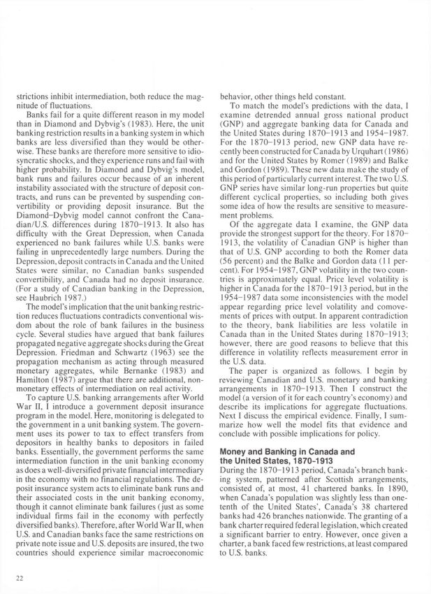
strictions inhibit intermediation, both reduce the mag-     behavior, other things held constant.
nitude of fluctuations.                                         To match the model's predictions with the data, I
    Banks fail for a quite different reason in my model     examine detrended annual gross national product
than in Diamond and Dybvig's (1983). Here, the unit         (GNP) and aggregate banking data for Canada and
banking restriction results in a banking system in which    the United States during 1870-1913 and 1954-1987.
banks are less diversified than they would be other-        For the 1870-1913 period, new GNP data have re-
wise. These banks are therefore more sensitive to idio-     cently been constructed for Canada by Urquhart (1986)
syncratic shocks, and they experience runs and fail with    and for the United States by Romer (1989) and Balke
higher probability. In Diamond and Dybvig's model,          and Gordon (1989). These new data make the study of
bank runs and failures occur because of an inherent         this period of particularly current interest. The two U.S.
instability associated with the structure of deposit con-   GNP series have similar long-run properties but quite
tracts, and runs can be prevented by suspending con-        different cyclical properties, so including both gives
vertibility or providing deposit insurance. But the         some idea of how the results are sensitive to measure-
Diamond-Dybvig model cannot confront the Cana-              ment problems.
dian/U.S. differences during 1870-1913. It also has             Of the aggregate data I examine, the GNP data
difficulty with the Great Depression, when Canada           provide the strongest support for the theory. For 1870-
experienced no bank failures while U.S. banks were           1913, the volatility of Canadian GNP is higher than
failing in unprecedentedly large numbers. During the        that of U.S. GNP according to both the Romer data
Depression, deposit contracts in Canada and the United      (56 percent) and the Balke and Gordon data (11 per-
States were similar, no Canadian banks suspended            cent). For 1954-1987, GNP volatility in the two coun-
convertibility, and Canada had no deposit insurance.        tries is approximately equal. Price level volatility is
(For a study of Canadian banking in the Depression,         higher in Canada for the 1870-1913 period, but in the
see Haubrich 1987.)                                          1954-1987 data some inconsistencies with the model
   The model's implication that the unit banking restric-   appear regarding price level volatility and comove-
tion reduces fluctuations contradicts conventional wis-     ments of prices with output. In apparent contradiction
dom about the role of bank failures in the business         to the theory, bank liabilities are less volatile in
cycle. Several studies have argued that bank failures       Canada than in the United States during 1870-1913;
propagated negative aggregate shocks during the Great       however, there are good reasons to believe that this
Depression. Friedman and Schwartz (1963) see the            difference in volatility reflects measurement error in
propagation mechanism as acting through measured            the U.S. data.
monetary aggregates, while Bernanke (1983) and                 The paper is organized as follows. I begin by
Hamilton (1987) argue that there are additional, non-       reviewing Canadian and U.S. monetary and banking
monetary effects of intermediation on real activity.        arrangements in 1870-1913. Then I construct the
   To capture U.S. banking arrangements after World         model (a version of it for each country's economy) and
War II, I introduce a government deposit insurance          describe its implications for aggregate fluctuations.
program in the model. Here, monitoring is delegated to      Next I discuss the empirical evidence. Finally, I sum-
the government in a unit banking system. The govern-        marize how well the model fits that evidence and
ment uses its power to tax to effect transfers from         conclude with possible implications for policy.
depositors in healthy banks to depositors in failed
banks. Essentially, the government performs the same        Money and Banking in Canada and
intermediation function in the unit banking economy         the United States, 1870-1913
as does a well-diversified private financial intermediary   During the 1870-1913 period, Canada's branch bank-
in the economy with no financial regulations. The de-       ing system, patterned after Scottish arrangements,
posit insurance system acts to eliminate bank runs and      consisted of, at most, 41 chartered banks. In 1890,
their associated costs in the unit banking economy,         when Canada's population was slightly less than one-
though it cannot eliminate bank failures (just as some      tenth of the United States', Canada's 38 chartered
individual firms fail in the economy with perfectly         banks had 426 branches nationwide. The granting of a
diversified banks). Therefore, after World War II, when     bank charter required federal legislation, which created
U.S. and Canadian banks face the same restrictions on       a significant barrier to entry. However, once given a
private note issue and U.S. deposits are insured, the two   charter, a bank faced few restrictions, at least compared
countries should experience similar macroeconomic           to U.S. banks.

22
Stephen D. Williamson
   Bank Failures

Chart 1
Percentage Deviations From Trend of U.S. Output and Bank Failures, 1870-1913*

                               1870          1875          1880          1885          1890          1895          1900          1905          1910

                           'Computed using a Hodrick-Prescott filter (see Prescott 1983). For bank failures, the percentage deviations are divided by 10.
                           Sources of basic data: Romer 1989, U.S. Department of Commerce 1975

   The government of Canada had a monopoly on the                                                   In the same period, the United States had a unit
issue of small-denomination notes during 1870-1913,                                              banking system, as it still does today. There were few
but circulating currency in large denominations con-                                             barriers to entry in the banking industry, but banks
sisted mostly of bank notes (Johnson 1910). Canadian                                             faced numerous restrictions, which tended to keep
banks could issue notes in denominations of $4 and                                               them small and limit diversification. In 1890, the
more (raised to $5 in 1880). A bank's note issue was                                             United States had about 8,200 banks, including nearly
limited by its capital, but this constraint does not seem                                        3,500 national banks (U.S. Department of Commerce
to have been binding on the system as a whole through                                            1975). Circulating paper currency consisted mainly of
most of the period.1 There was a limited issue of                                                national bank notes (in denominations of $ 1 and more)
Dominion notes (federal government currency), backed                                             and notes issued directly by the U.S. Treasury. National
25 percent by gold and 75 percent by government                                                  bank notes were more than fully backed by federal
securities, with additional issues backed 100 percent by                                         government bonds at the time of issue and were guar-
gold. Legislation periodically increased the limit on the                                        anteed by the federal government. All banks were
fractionally gold-backed component of government-                                                subject to reserve requirements.
issued currency.                                                                                    During the National Banking Era, the U.S. banking
   There were no Canadian reserve requirements,2 but                                             system was subject to recurrences of widespread panic
after 1890, 5 percent of note circulation was held on                                            and bank failure, as is well known. Pervasive financial
deposit in a central bank circulation redemption fund.
This added insurance was essentially redundant, since                                                'In 1907, this constraint on note issue appears to have become binding
notes were made senior claims on bank assets in 1880.                                           during the crop-moving season. At that time, the Canadian government
                                                                                                instituted a temporary rediscounting arrangement with the banks. The arrange-
Most bank notes appear to have circulated at par,                                               ment was made permanent with the Finance Act of 1914.
especially after 1890 legislation that required redemp-                                             2
                                                                                                      If reserves were held, one-third (40 percent after 1880) had to be held in
tion of notes in certain cities throughout Canada.                                              the form of Dominion notes.

                                                                                                                                                                             23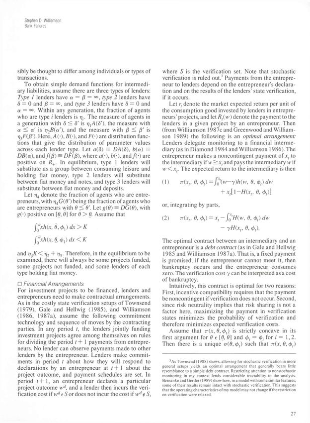
crises occurred in 1873, 1884, 1890, 1893, and 1907
(Sprague 1910). Chart 1 plots percentage deviations         Table 1
from trend in GNP and in bank suspensions in the            Canada's 23 Chartered Bank Liquidations, 1870-1913
United States between 1870 and 1913. There is clearly
negative comovement, with a correlation coefficient of
—0.25, between the series. Friedman and Schwartz                                                                 % of Face Value of
(1963) and Cagan (1965) also find that panic periods                                                            Bank Liabilities Paid to
tend to be associated with declines in real output growth             Year of           Bank Liabilities at
                                                                      Suspension       Suspension (Can. $)    Noteholders      Depositors
and with increases in the currency-to-deposit ratio.
   The striking difference in the incidence of bank                   1873                    106,914               .00            .00
failure in Canada and the United States during the                    1876                  293,379             100.00          100.00
Great Depression has been noted by Friedman and                       1879                  547,238              57.50           57.50
Schwartz (1963) and Bernanke (1983) and studied by                                          136,480             100.00           96.35
Haubrich (1987). Between 1923 and 1985, no Cana-                                          1,794,249             100.00          100.00
dian banks failed; but from 1930 to 1933, more than
                                                                                            340,500             100.00          100.00
9,000 U.S. banks suspended operations. The record of
                                                                      1881                1,108,000              59.SO           59.50
bank failures in the two countries during 1870-1913,
while showing less striking differences than in the                   1883                2,868,884             100.00           66.38
Depression, also indicates that the incidence of bank                 1887                1,409,482             100.00           10.66
failure was lower and the disruptive effects of bank                                         74,364             100.00          100.00
failures were much smaller in Canada than in the                                          1,031,280             100.00          100.00
United States.                                                                            2,631,378             100.00           99.66
    Evidence supporting these observations appears in                 1888                3,449,499             100.00          100.00
Table 1, which displays statistics on bank liquidations               1893                1,341,251             100.00          100.00
in Canada during 1870-1913. In total, Canada had                      1895                7,761,209             100.00           75.25
23 bank liquidations while, at the same time, the United              1899                1,766,841             100.00           17.50
States had 3,208. This evidence, however, clearly
                                                                      1905                  388,660             100.00          100.00
overstates the difference between Canadian and U.S.
                                                                      1906               15,272,271             100.00          100.00
bank failure rates, since Canadian banks were larger
than U.S. banks and since Canadian GNP and popula-                    1908               16,174,408             100.00          100.00
tion were less than one-tenth of the corresponding                                          560,781             100.00           30.27
quantities in the United States over the period. Thus,                                    1,172,630             100.00          100.00
the failure of an average-sized Canadian bank would                   1910                  549,830             100.00          100.00
potentially have had a much larger effect on the                                          1,997,041             100.00             .00
Canadian economy than the failure of an average-sized
                                                                 Source: Beckhart 1929 (pp. 4 8 0 - 8 1 )
U.S. bank would have had on the U.S. economy.
   According to Table 1, noteholders of failed banks
received 100 percent of the face value of their liabili-
                                                                Further, Canadian chartered banks had cooperative
ties in 20 of the 23 Canadian bank liquidations, and
                                                            arrangements that tended to lessen the adverse effects
depositors received 100 percent in 12 of the 23. This
might indicate relatively little economic disruption        of bank failures. Canadian banks were mainly self-
from Canadian bank failures, but that conclusion            regulated, with a formal organization, the Canadian
requires comparable statistics for the United States.       Bankers' Association, established in 1891 and given
These are provided in Table 2, which displays some          special powers through legislation in 1900. The largest
data on bank depositors' losses in Canada and the           banks, particularly the Bank of Montreal, appear to
United States. On average, in the years under study,        have been willing to act as informal lenders of last
losses to depositors were 0.07 percent of total deposits    resort and to step in to help reorganize troubled banks.
in Canada and 0.11 percent in the United States. By this    This excerpt from Johnson (1910, pp. 124-25) is
measure, the disruption from bank failures appears to       illustrative:
have been significantly smaller—57 percent smaller—            On the evening of October 12 [1906] the bankers in
in Canada than in the United States.                           Toronto and Montreal heard with surprise that the Bank of

24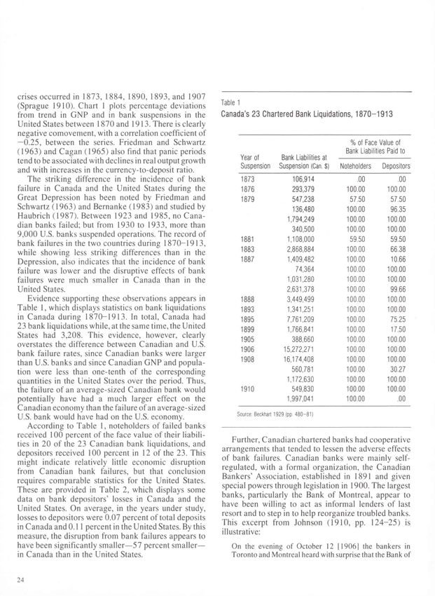
Stephen D. Williamson
   Bank Failures

                                                                                bank, but none of them took alarm and many of them were
Table 2
                                                                                well pleased with the change.
Bank Depositor Losses as a Percentage
of Total Deposits                                                               The collective behavior of Canadian banks not only
                                                                             served to minimize the costs of liquidating insolvent
                                                                             institutions; it also appears to have prevented wide-
                                                                             spread banking panics. Any bank runs seem to have
            Country and Year                         Annual Percentage*
                                                                             been confined to individual banks or branches (U.S.
                                                                             Congress 1910). Although U.S. banks had cooperative
            Canada**
                                                                             arrangements during the National Banking Era, par-
               1873                                            .03%          ticularly clearinghouses (Gorton 1985), the ability of
               1879                                            .15
                                                                             U.S. banks to act as a single coalition could not ap-
               1881                                            .20
               1883                                            .69
                                                                             proach that of their Canadian counterparts.
               1887                                            .87
               1895                                            .89           T h e Model
               1899                                            .47           I now construct a model that captures the essential
               1908                                            .04           features of the banking and monetary structures of
               1910                                            .14
                                                                             Canada and the United States during the 1870-1930
               1914                                            .05
                                                                             period.
               1867-1920                                       .07%              I have already described two important differences
                                                                             between Canadian and U.S. banking and monetary
           United States                                                     arrangements at that time. One is that Canadian bank
               1865-1880                                       .19%          liabilities were much less subject to idiosyncratic risk
               1881-1900                                       .12           than were U.S. bank liabilities. The Canadian system let
               1901-1920                                       .04           Canadian banks become larger than U.S. banks, and
               1865-1920                                       .11%          branch banking allowed greater geographical diversi-
                                                                             fication. Further, the cooperative behavior among
            *For multiyear spans, average annual losses as a percentage of   Canadian banks helped to insure depositors against
            deposits were computed first and then averaged.                  losses. The second important difference is related to
           '"For years not included, the annual percentage of losses to
                                                                             the fact that Canadian banks could issue circulating
            deposits was zero.
            Sources: Beckhart 1929, FDIC 1941
                                                                             notes in large denominations and back them with
                                                                             private assets. In the United States, only national banks
                                                                             could issue notes, and these notes had to be backed
                                                                              111 percent by U.S. government bonds. Thus, Canadian
    Ontario had got beyond its depth and would not open its                  bank notes could perform an intermediation function
    doors the next morning. . . . The leading bankers in the                 whereas U.S. bank notes could not (to the extent that
    Dominion dreaded the effect which the failure of such a
                                                                             breaking government bonds into small denominations
    bank might have. The Bank of Montreal agreed to take
    over the assets and pay all the liabilities, provided a
                                                                             is an insignificant function compared to the intermedia-
    number of other banks would agree to share with it any                   tion normally done by banks).
    losses. Its offer was accepted and a representative of the                   The model should be able to replicate the differences
    Bank of Montreal took the night train for Toronto. Going                 of the Canadian and U.S. experiences with regard to
    breakfastless to the office of the Bank of Ontario he found              bank failures. That is, bank failures should be nega-
    the directors at the end of an all-night session and laid                tively correlated with aggregate activity, and the inci-
    before them resolutions officially transferring the business             dence of bank failure should be higher in the model U.S.
    and accounts of the bank to the Bank of Montreal. They                   economy than in the model Canadian economy.
    adopted the resolution before 9 a.m. and the bank opened
    business for the day with the following notice over the
                                                                                 The model constructed here is related to the models
    door: "This is the Bank of Montreal."                                    of Williamson (1987c) and Greenwood and Williamson
        Before 1 o'clock the same notice, painted on a board or              (1989) but differs from them somewhat to capture the
    penciled on brown wrapping paper, was over the door of                   problem at hand. The model abstracts from reserve
    the 31 branches in different parts of the Dominion. Its                  requirements, interest-bearing government debt, and
    customers were astonished that day when they went to the                 the operation of the gold standard monetary regime.

                                                                                                                                    25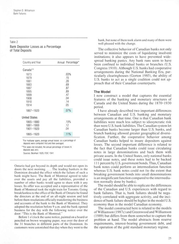
The Canadian         Economy                                           D 3 //(jt, 0, 0) = 0            for w > K
•    Environment
                                                                       j"xD3h(x}   0, 0) dx = 0.
The Canadian economy is modeled as a closed econ-
omy with a continuum of two-period-lived agents born               Assume that the aggregate shock 0, follows a two-
in each period t = 1,2,3,        The measure of a               state Markov process. That is, 0, = 0,- for i— 1,2, and
generation is N. Each generation has two types of               Pr[0, +1 = 0, 10, = 0,] = qx for / = 1,2, where 0  0 , f o r / = 1,2 and qx > q2. Aggregate shocks
each receive an indivisible endowment of one unit of            are therefore nonnegatively serially correlated, and all
time when young and maximize                                    project returns are riskier in state 2 than in state 1.
                                                                   Project returns are independently distributed across
                                                                entrepreneurs. There is costly state verification (as in
                                                                Townsend 1979, 1988). That is, entrepreneurs can
where                                                           observe the return on their own project w, but any other
                                                                agent expends y units of effort to observe w.
        Et = the expectation operator conditional
                                                                   Lenders who choose to produce the consumption
              on period t information
                                                                good in period t save the entire amount by acquiring fiat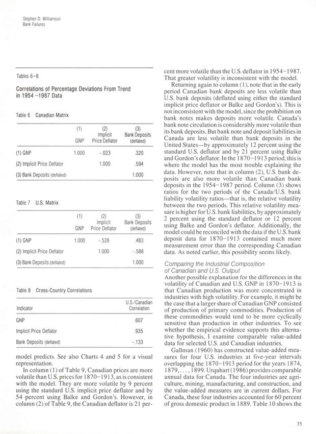
Stephen D. Williamson
   Bank Failures

sibly be thought to differ among individuals or types of        where S is the verification set. Note that stochastic
transactions.                                                   verification is ruled out.3 Payments from the entrepre-
   To obtain simple demand functions for intermedi-             neur to lenders depend on the entrepreneur's declara-
ary liabilities, assume there are three types of lenders:       tion and on the results of the lenders' state verification,
Type 1 lenders have a = (3 = 00, type 2 lenders have            if it occurs.
6 = 0 and p = 00 , and type 3 lenders have 5 = 0 and                Let rt denote the market expected return per unit of
a = 00 . Within any generation, the fraction of agents          the consumption good invested by lenders in entrepre-
who are type i lenders is 77, . The measure of agents in        neurs' projects, and let Rt(w) denote the payment to the
a generation with K                                                             - yH(xr 0, ,).

        {™xh(x, 0,x)dx, = (f>i for i = 1,2.
for dividing the period t + 1 payments from entrepre-           Then there is a unique a(0, t) such that 7r(x, 0, ,)
neurs. No lender can observe payments made to other
lenders by the entrepreneur. Lenders make commit-
ments in period t about how they will respond to                     3
                                                                       As Townsend (1988) shows, allowing for stochastic verification in more
                                                                general setups yields an optimal arrangement that generally bears little
declarations by an entrepreneur at t + 1 about the              resemblance to a simple debt contract. Restricting attention to nonstochastic
project outcome, and payment schedules are set. In              monitoring in my context lends considerable tractability to the analysis.
period t + 1, an entrepreneur declares a particular             Bernanke and Gertler (1989) show how, in a model with some similar features,
                                                                some of their results remain intact with stochastic verification. This suggests
project outcome wd, and a lender then incurs the veri-          that the operating characteristics of my model may not change if the restriction
fication cost if wd e S or does not incur the cost if wd q 5,   on verification were relaxed.

                                                                                                                                             27
reaches a maximum for x = ct(0,with fixed 0 and , lender, indifferent between holding intermediary notes
and a(0,r) e (0, vv). Entrepreneurs for whom and holding fiat money, has rt~ a = EtpJ+xlpr And
7r(cj(0, ,), 0, ,) > receive loans, while those the type 3 lender, indifferent between holding inter-
with 7r(a(0, ,), < do not. For the entre- mediary deposits and holding fiat money, has rt — (3 =
preneurs receiving loans, the promised payment xt Etpt+Xlpr Equilibrium in the market for fiat money
satisfies therefore implies that
(3) 7T (xr6^t) = rtK. (8) r]xA(Etpt+x/pt)
Note that xt decreases with 0; that is, the loan interest + rj2[l-B(rrEtpt+x/pt)]
rate is lower for higher-quality projects. + rj3[ 1 —F(r—Etpt+ {/pt)] = ptM0
Financial intermediaries are those type 3 lenders
with (3 = 0. These intermediaries can commit to making where the left side of (8) is the demand for fiat money
noncontingent payments of rt to each of their depositors (with the three terms representing the demand for fiat
and noteholders by holding large portfolios and achiev- money by type 1, type 2, and type 3 lenders, respec-
ing perfect diversification.4 Since each of an inter- tively) and the right side of (8) is the supply of fiat
mediary's depositors and noteholders receives rt with money. In the credit market, equilibrium implies that
certainty, the liability holders never need to monitor the
intermediary.
(9) r]2B(rrEtpt+x/pt) + r]3F(rrEtpt+x/pt)
This optimal arrangement captures some important
features of financial intermediation arrangements = r; 4 K[l-G(0/)]
observed in the real world. In the model, intermediaries
diversify, transform assets, process information, and where the first term on the left side of (9) is credit
hold debt in their portfolios. supplied (through financial intermediaries) by note-
holders, the second term on the left side is credit
• Equilibrium supplied by intermediary depositors, and the right side
In equilibrium, there is some 6't such that entrepreneurs is credit demanded by entrepreneurs.
with 0 > Q't receive loans while those with 0 < 0't do not. Now restrict attention to the stationary monetary
Let x\ denote the promised payment for the marginal equilibrium, where pt> 0 for all t and quantities and
borrower; that is, x\ — o(0'r ,). Then prices depend only on the state r Let subscripts denote
the state. Then
(4) 7r(x't, 0'r t) = rtK
(10) Etpt+X = q{px + ( 1 -qt)p2
(5) Dx Hx;, 0,', ,) = 0.
for (j>t = 4>i and i — 1,2. Let 5" = px/p2. Then from (8),
Since 7r(% % •) is concave in its first argument, equations (9), and (10) come
(4) and (5) solve for x't and Q't given rv Using (2) to
substitute in (4) and (5) gives
(11) rjxA(q{+(l-q{)/s)
(6) x\ - f*'H(w, 0;, ,) dw - yH(x'r 0;, 4>t) — rtK + rj2[l-B(rrq-(l-qx)/s)]
(7) 1 - H(x'v 0;, ,) - yh(x'v 0;, 0,) = 0. + rh[\-F(r-q-(\-qx)/s)]
-s{r]xA(q2s+l-q2)
Given the market expected return rv (6) and (7)
determine x\ and 6[. + rj2[\-B(r2-q2s~l+q2)]
Let pt denote the price of fiat money in period t, in + V3[l-F(r2-q2s-l+q2)]} =0
terms of the consumption good. The expected return on
fiat money in period t is then Etpt+l/pr The type 1
lender, who is indifferent between consuming leisure 4
Formal arguments rely on the law of large numbers (Williamson
and producing the consumption good to exchange for 1986,1987c), though there are some subtleties here because of the continuum
fiat money, has 5 = Etpt+x/pr Similarly, the type 2 of agents.
28Stephen D. Williamson Bank Failures (12) ri2B
(22)    7r*(jt,*(0), 6, 4>t) = r*K.                           and the underlying disturbance () evolves in an analyti-
                                                              cally convenient way (as a Markov process). As a result
The number of banks that fail in period t + 1 is then         it is easy, using calculus, to derive algebraic formulas
                                                              for the variances and covariances of key variables.
(23)             = N*l0e;. H(x*(d\ 6, ,)g(0) rffl.             As shown rigorously in Williamson 1989, fluctua-
                                                              tions in the two economies are qualitatively similar. In
    The contractual arrangement with unit banking can         both countries, bank liabilities (bank notes plus de-
be interpreted as involving a bank run when a bank            posits) and the price level (the inverse of the price of fiat
failure occurs. That is, the verification cost y could        money) are procyclical. That is, each of these variables
represent the cost to each depositor of getting to the        and output are mutually positively correlated. Thus, if
bank early to withdraw a deposit. On receiving a signal       both economies are subjected to the same real distur-
at the beginning of period t + 1 that failure is imminent,    bances, they experience business cycles that move in
each depositor incurs the cost of running to the bank,        phase. The mean-preserving spread in the distribution
each receives less than the promised return, and the          of investment project returns that occurs in state 2 can
bank fails. Runs are never observed when banks are            be thought of as a decrease in the demand for credit.
perfectly diversified, because then depositors would          This disturbance causes the real interest rate r and the
never need to verify the return on the bank's portfolio.      quantity of credit extended by intermediaries to fall
    With this interpretation of bank runs and failures,       in state 2 relative to state 1. This credit decrease is
this model seems better able to confront U.S. and             matched by a decrease in the quantity of bank lia-
Canadian experience than the bank runs model of               bilities, so the demand for fiat money rises and the price
Diamond and Dybvig (1983) or the related model of             level falls. Output tends to be higher in state 1 than in
Postlewaite and Vives (1987). These other models rely         state 2 for two reasons. One is that the expected real rate
on inherent features of the deposit contract to explain       of return on fiat money is higher in state 1, so lenders
runs, which leaves the very different behavior of the         work more and consume less leisure. The other reason
U.S. and Canadian banking systems unexplained.                is that since the shock , is positively serially correlated,
                                                              a period with a high quantity of credit extended is
                                                              followed by state 1 with higher probability than by state
Model Implications                                            2. Thus, output from the previous period's investment
I now explore some of the model's implications for the        tends to be higher in state 1 than in state 2.
interaction between financial structure and macroeco-
nomic fluctuations.                                               The perturbation has two effects on the volatility of
                                                             U.S. bank failures. First, the number of failures tends to
For Aggregate          Fluctuations                          be larger in state 2 because entrepreneurs with the same
Having characterized an equilibrium in equations (11)-       characteristics (the same 0) and who receive loans in
(15) for the Canadian economy and in (16)—(21) for           states 1 and 2 face a higher promised payment x*(0) in
the U.S. economy, I proceed to analyze aggregate             state 2 (the state where investment projects are riskier).
fluctuations in the two economies. This analysis is          In state 2, therefore, banks that fund projects of the
carried out by determining the qualitative comove-           same quality have a higher probability of failing than
ments among key aggregate variables in each economy          in state 1. Second, since 0'* is higher in state 1 than in
and making quantitative comparisons across the two.          state 2, the average quality of projects (without taking
(The methods used to do this are detailed in Williamson      account of the change in riskiness) is lower in state 1.
1989.)                                                       This tends to make the number of failures larger in state
    I use the following approach: For each economy,          1 than in state 2. The first effect tends to induce
start with a benchmark equilibrium in which there are        countercyclical bank failures; the second, procyclical
no fluctuations—that is, where there are no shocks           bank failures. It seems reasonable to assume that the
(, =  for all t) with s=l, r{=r2 = r, and d[ = 02 — 0' first effect dominates, so that bank failures are counter-
in the Canadian economy, and similarly for the U.S.          cyclical, as is true in the U.S. data for this period.
economy. Then, subject the two parallel economies to a            The next step is to make a quantitative comparison
small perturbation around the benchmark equilibrium.         of fluctuations in the two economies. (Again, the details
We now have ! =  and 2 > , where 2 — 1 is appear in Williamson 1989.) The effect of the unit
small. The perturbations to the benchmark equilibrium        banking restriction and of the prohibition on private
are small, the economy can be only in one of two states,     bank note issue (each considered separately) is to make

30
Stephen D. Williamson
Bank Failures
Charts 2 and 3
How Two Restrictions Affect Fluctuations Induced by Project Risk in the Credit Market
Chart 2 Unit Banking Restriction Chart 3 Prohibition on Private Bank Notes
Interest Demand for Credit Interest Supply of Credit
Rate (r) Rate (r) With Prohibition
With Unit
Banking Only on Notes
D Supply Demand ;
Sl With No Prohibition
With Perfect
of Credit for Credit / on Notes
L
Diversification
D, _/ s o
D ° \
X —^
\
\ "
/ /i \
1 \ / /1 \
r /i \
/ r v / i \
/ i V l \
\ X
/ • • \
1 ^
i i
i i
Quantity Quantity
of Credit of Credit
K
per capita bank liabilities, per capita output, and the projects financed, and output (in the subsequent period)
price level less variable. Though the unit banking fall. With the imposition of a unit banking system, the
restriction makes bank deposits less variable, deposits credit demand curve becomes less elastic. That is, if an
become more variable with a prohibition on private entrepreneur defaults, the verification costs incurred by
note issue. lenders are now yK rather than K, so expected verifi-
Some partial equilibrium intuition may clarify the cation costs increase more rapidly as the quality of
forces that produce these results. Ignoring the dynamic investment projects (0) decreases. An increase in riski-
effects from movements in the price level, think of the ness for all projects thus shifts D{ to Dp and the change
model in terms of credit supply and demand, where the in the interest rate and the quantity of projects financed
competitively determined price is the interest rate r. In is smaller than with perfect diversification.
Chart 2, the credit demand curve D 0 is determined by The effect of a prohibition on private bank notes is
the number of investment projects that, if funded, will shown in Chart 3. As the supply of credit becomes less
yield a return per lender of at least r. Credit supply is elastic (S0 shifts to Sj), agents who would otherwise
determined by the number of lenders who hold inter- hold intermediated assets instead hold unproductive
mediary liabilities for each r. With branch banking and fiat currency. When risk increases for all projects
no prohibition on bank note issue, an increase in the (shifting D0 to DQ), the quantity of credit falls less than
riskiness of investment projects shifts the demand curve it would have otherwise. Thus, credit, bank liabilities,
to DQ, since fewer projects are now creditworthy for and output are more volatile when private bank note
each r. As a result the interest rate, the quantity of issue is permitted.
31In the model, disturbances that make credit more ments since World War II can be viewed as equivalent.
volatile also tend to make prices more volatile since, With the establishment of the Bank of Canada in 1935,
with a fixed nominal stock of currency, the price level private bank note issue was prohibited in Canada, and
equates the supply of and the demand for fiat money. Canadian banks were, if anything, larger and better
When private bank note issue is permitted, deposits diversified after the war than before. The U.S. deposit
tend to be less volatile because the interest rate is less insurance system can be seen as accomplishing a
volatile and because price movements induce more function similar to that of a well-diversified banking
substitution into fiat currency from deposits. system; the only difference is that in the U.S. system,
The fact that the unit banking restriction induces less monitoring is delegated partly to the government rather
volatility in aggregate activity is perhaps surprising. In than entirely to private financial intermediaries. The
the model U.S. (unit banking) economy, countercyclical model constructed here, then, predicts that, other things
bank failures are observed. Relaxing this restriction in held constant, aggregate fluctuations should have sim-
the model makes bank failures a constant (that is, zero). ilar properties across the two countries in the postwar
Thus, intuition might suggest that aggregate volatility period.
should be smaller in the model Canadian economy with
perfectly diversified banks. But the model contradicts The Empirical Evidence
this intuition.
The model also seems at odds with the views of Comparing Canadian and U.S. Data
Friedman and Schwartz (1963), Bernanke (1983), and I now examine annual aggregate data for Canada and
Hamilton (1987). Friedman and Schwartz assign an the United States for the periods 1870-1913 and
important macroeconomic role to bank failures in the 1954-1987. I attempt to discover whether the evi-
United States during the Depression, a role they think dence is consistent with the model and its implications.
operated through reductions in measured monetary The aggregate data come from several sources. For
aggregates. Bernanke and Hamilton argue that bank Canada from 1870-1913, Urquhart (1986) construc-
failures in the Depression had effects other than those ted series for constant dollar GNP and the implicit price
reflected in monetary aggregates. However, note that deflator. He used a value-added method to assemble the
both Bernanke (1983, pp. 266-67) and Friedman and GNP data, and the resulting series seems to be consider-
Schwartz (1963, pp. 352-53) have difficulty reconcil- ably better than the U.S. data available for this period.
ing their views with Canadian experience in the For U.S. constant dollar GNP in 1870-1913,1 use two
Depression. During this time, Canada and the United alternative series constructed by Romer (1989) and
States experienced comparable declines in output, but Balke and Gordon (1989). They used similar regression
no Canadian banks failed (Haubrich 1987). methods but different underlying data. These series
seem to be the best existing measures of U.S. GNP for
With Deposit Insurance this period. They have similar low frequency properties,
Government deposit insurance programs have played but their cyclical properties are different. For implicit
an important role in discussions of banking insta- price deflators for 1870-1913, I use a standard his-
bility—for example, in Diamond and Dybvig 1983. torical series from Balke and Gordon 1986 and an
Such a program can be introduced into the model's unit updated series from Balke and Gordon 1989. Data on
banking system as follows. Assume the government is chartered bank deposits and bank notes in circulation in
an agent that can supply effort to monitor entrepre- Canada in 1870-1913 come from monthly statements
neurs. The government guarantees all bank depositors by the chartered banks, published in the Canada Year
a certain return in each period. If a bank fails, the Book (1915). Data on U.S. commercial bank deposits
government verifies the return on the bank's portfolio. are from Friedman and Schwartz (1970), but these are
Lump-sum taxes are levied, either on banks or on inferior to the Canadian data, since the U.S. series was
depositors. The taxes are just sufficient to compensate constructed from national banks' infrequent call reports
depositors in failed banks and to compensate the and from scant state bank data. For 1954-1987, data
government for effort expended in monitoring banks. come from the C ANSIM data base, the Federal Reserve
This arrangement yields an equilibrium allocation Board data base, and the FDIC Annual Report (various
identical to the one achieved with perfectly diversified years).
banks. All time series were subjected to a log transforma-
Canadian and U.S. banking and monetary arrange- tion and were detrended using a Hodrick-Prescott filter
32Stephen D. Williamson
Bank Failures
(Prescott 1983), which essentially fits a smooth, time-
Tables 3 - 5
varying trend to the data.5 Multiplying the resulting
series by 100 gives time series that are percentage
deviations from trend. The model yields predictions Correlations of Percentage Deviations From Trend
in 1870-1913 Data
about unconditional variances and covariances of per
capita aggregates in economies that do not grow. Thus,
the data transformations account as well as seems Table 3 Canadian Matrix
possible for differences between the two countries in
long-run growth, scale, and population.
(1) (2) (3) (4) (3)+(4)
Tables 3 and 4 show correlation matrixes for per- Gross Implicit Bank Bank Bank
centage deviations from trend of the Canadian and U.S. National Price Deposits Notes Liabilities
data in 1870-1913. Table 5 shows cross-country Product Deflator (deflated) (deflated) (deflated)
correlations. Also see Chart 4. Tables 3 and 4 are
generally consistent with the model, in that all but one (1) 1.000 .475 .433 .717 .588
of the series are mutually positively correlated in both
countries. In addition, Table 5 shows a high degree of (2) 1.000 -.026 .522 .182
correlation between corresponding variables in the two 1.000 .491 .941
(3)
countries. This is consistent with the assumption that
real disturbances common to both countries dominate (4) 1.000 .748
over this period.
(3)+(4) 1.000
Tables 6, 7, and 8 show correlations for the period
1954-1987 and correspond to Tables 3,4, and 5. Also
see Chart 5. Tables 6 and 7 indicate some inconsis-
tencies with the model. In the Canadian data, there is
Table 4 U.S. Matrix
essentially no correlation between GNP and the price
level, and in the U.S. data, the GNP/price level and
price level/bank deposit correlations are negative. Also, (1) (2) (3) (4)
GNP GNP Implicit Bank
in Table 8, U.S. and Canadian bank deposits are nega- (Romer's (Balke & Price Deflator Deposits
tively correlated. There thus appear to be important Data) Gordon's Data) (standard) (deflated)
factors affecting aggregate fluctuations in Canada and
the United States in the later period that are not (1) 1.000 .691 .183 .217
captured in the model. Care is needed, therefore, in
interpreting the 1954-1987 data and in comparing the (2) 1.000 .502 .523
later period with the earlier one. (3) 1.000 .494
Table 9 shows standard deviations of the trans-
formed series for each time period, ratios of these (4) 1.000
volatility measures for Canada and the United States
for each period, and volatility ratios for the two periods.
Perhaps the strongest evidence supporting the model's
predictions is in the volatility measures for the GNP Table 5 Cross-Country Correlations
data from both periods. From column (1), Canadian
GNP is considerably more volatile than U.S. GNP for U.S./Canada
the period 1870-1913. Volatility is 56 percent greater Indicator Correlation
using Romer's GNP data and 11 percent greater using
GNP
Balke and Gordon's. For 1954-1987, GNP volatility
With Romer's Data .395
is virtually identical in the two countries, as the
With Balke & Gordon's Data .678
Implicit Price Deflator .677
5
Here I set X, the parameter that governs the smoothness in the trend, to U.S. Bank Deposits/Canadian
400. An increase in X makes the trend smoother. Prescott (1983) uses Bank Notes + Deposits (all deflated) .518
X = 1,600 for quarterly data.
33Charts 4 and 5
Percentage Deviations From Trend of U.S. and Canadian Output (GNP)
Chart 4 In 1 8 7 0 - 1 9 1 3
Chart 5 In 1 9 5 4 - 1 9 8 7
%
A
United States
Canada
Jv
I
1955
I
1960
I
1965
I
1970
/vI
1975
1
1980
i
1985
Sources of basic data: Urquhart 1986, Romer 1989, CANSIM data base, Federal Reserve Board data base
34Stephen D. Williamson
Bank Failures
cent more volatile than the U.S. deflator in 1954-1987.
Tables 6 - 8 That greater volatility is inconsistent with the model.
Returning again to column (1), note that in the early
Correlations of Percentage Deviations From Trend period Canadian bank deposits are less volatile than
in 1954 -1987 Data U.S. bank deposits (deflated using either the standard
implicit price deflator or Balke and Gordon's). This is
not inconsistent with the model, since the prohibition on
Table 6 Canadian Matrix
bank notes makes deposits more volatile. Canada's
bank note circulation is considerably more volatile than
(2) (3) its bank deposits. But bank note and deposit liabilities in
Implicit Bank Deposits
Canada are less volatile than bank deposits in the
GNP Price Deflator (deflated)
United States—by approximately 12 percent using the
(1) GNP 1.000 -.023 .320 standard U.S. deflator and by 21 percent using Balke
and Gordon's deflator. In the 1870-1913 period, this is
(2) Implicit Price Deflator 1.000 .594 where the model has the most trouble explaining the
data. However, note that in column (2), U.S. bank de-
(3) Bank Deposits (deflated) 1.000
posits are also more volatile than Canadian bank
deposits in the 1954-1987 period. Column (3) shows
ratios for the two periods of the Canada/U.S. bank
liability volatility ratios—that is, the relative volatility
Table 7 U.S. Matrix between the two periods. This relative volatility mea-
sure is higher for U.S. bank liabilities, by approximately
(1) (2) (3) 2 percent using the standard deflator or 12 percent
Implicit Bank Deposits using Balke and Gordon's deflator. Additionally, the
GNP Price Deflator (deflated)
model could be reconciled with the data if the U.S. bank
(1) GNP 1.000 -.528 .483
deposit data for 1870-1913 contained much more
measurement error than the corresponding Canadian
(2) Implicit Price Deflator 1.000 -.588 data. As noted earlier, this possibility seems likely.
(3) Bank Deposits (deflated) 1.000 Comparing the Industrial Composition
of Canadian and U.S. Output
Another possible explanation for the differences in the
volatility of Canadian and U.S. GNP in 1870-1913 is
Table 8 Cross-Country Correlations that Canadian production was more concentrated in
industries with high volatility. For example, it might be
U.S./Canadian the case that a larger share of Canadian GNP consisted
Indicator Correlation of production of primary commodities. Production of
these commodities would tend to be more cyclically
GNP .607 sensitive than production in other industries. To see
whether the empirical evidence supports this alterna-
Implicit Price Deflator .935
tive hypothesis, I examine comparable value-added
Bank Deposits (deflated) -.133 data for selected U.S. and Canadian industries.
Gallman (1960) has constructed value-added mea-
model predicts. See also Charts 4 and 5 for a visual sures for four U.S. industries at five-year intervals
representation. overlapping the 1870-1913 period for the years 1874,
In column (1) of Table 9, Canadian prices are more 1 8 7 9 , . . . , 1899. Urquhart( 1986) provides comparable
volatile than U.S. prices for 1870-1913, as is consistent annual data for Canada. The four industries are agri-
with the model. They are more volatile by 9 percent culture, mining, manufacturing, and construction, and
using the standard U.S. implicit price deflator and by the value-added measures are in current dollars. For
54 percent using Balke and Gordon's. However, in Canada, these four industries accounted for 60 percent
column (2) of Table 9, the Canadian deflator is 21 per- of gross domestic product in 1889. Table 10 shows the
35Table 9
Volatility of Percentage Deviations From Trend in Two Countries and Two Periods
Standard Deviation
(1) (2) (D-H2)
Country and Indicator 1870-1913 1954-1987
Canada
Gross National Product 4.87 2.51 1.94
Implicit Price Deflator 3.84 4.42 .87
Bank Notes 9.22
Deposits 4.96 4.69 1.06
Liabilities (Notes + Deposits) 5.26 4.69 1.12
United States
Gross National Product
Romer 3.13 2.57 1.22
Balke & Gordon 4.37 2.57 1.70
Implicit Price Deflator
Standard 3.53 3.66 .96
Balke & Gordon 2.49 3.66 .68
Bank Deposits
Standard Deflator 5.96 5.20 1.15
Balke & Gordon Deflator 6.64 5.20 1.28
Canada -r- United States
Gross National Product
Romer 1.56 .98 1.59
Balke & Gordon 1.11 .98 1.13
Implicit Price Deflator
Standard 1.09 1.21 .90
Balke & Gordon 1.54 1.21 1.27
Bank Liabilities
Standard Deflator .88 .90 .98
Balke & Gordon Deflator .79 .90 .88
percentage of value added in each of the four industries much larger in 1899. However, this 1899 number
in Canada and the United States for the selected years. was temporarily enlarged by the Klondike gold rush
As anticipated, Canada had a larger portion of output in (Urquhart 1986). The portion of value added in con-
agriculture and a smaller portion in manufacturing than struction was consistently much smaller in Canada than
did the United States, and this difference persists in the United States.
through the sample period. The portion of value added Again using the Hodrick-Prescott detrending pro-
in mining was smaller in Canada than in the United cedure, I computed standard deviations of percentage
States through most of the period, but Canada's portion deviations from trend for current Canadian dollar
was slightly larger than the United States' in 1894 and value-added measures for the four Canadian industries
36Stephen D. Williamson
Bank Failures
Table 10
Percentage of Value Added in Four Canadian and U.S. Industries
Based on Current Canadian and U.S. Dollar Data
Industry and Country
Agriculture Mining Manufacturing Construction
Year Canada U.S. Canada U.S. Canada U.S. Canada U.S.
1874 51.6 46.9 1.6 2.8 36.1 38.4 10.7 12.0
1879 59.1 49.0 2.0 2.9 32.4 37.0 6.5 11.1
1884 49.5 40.0 1.7 2.8 37.9 43.0 10.9 14.2
1889 46.8 35.1 2.7 3.6 41.5 47.4 9.0 13.9
1894 48.9 33.8 4.1 3.7 41.1 46.0 6.0 16.6
1899 44.9 33.3 8.2 4.6 40.2 49.5 6.8 12.6
Sources: Urquhart 1986, Gallman 1960
Table 11
As an additional check of the alternative hypothesis,
Volatility of Percentage Deviations From Trend I constructed a counterfactual nominal GNP series for
of Value Added in Four Canadian Industries, Canada for 1870-1913. This was done as follows. Let
1870-1913 Yt denote nominal GNP and yit denote nominal value
Based on Current Canadian Dollar Data added in industry i, where i— 1 , 2 , 3 , 4 for agriculture,
mining, manufacturing, and construction, respectively.
Again, an asterisk (*) superscript denotes a U.S.
variable. Then, counterfactual Canadian nominal GNP
Industry Standard Deviation (what Canadian GNP would have been with the same
relative composition of output as the United States in
Agriculture 8.2 agriculture, mining, manufacturing, and construction),
Mining 13.8 denoted Ytc} is computed as
Manufacturing 11.7
Construction 18.4
All Four Industries 9.0 The weights for i = 1, 2, 3, 4, were constructed as
follows:
Source of basic data: Urquhart 1986
* i t =(yVZUyO/(yj2Uyis)
in 1870-1913. These statistics are displayed in Table where s = 1 8 7 4 f o r / = 1 8 7 0 , . . . , 1876; 5 = 1879 for
11. Surprisingly, volatility was lowest in agriculture, t = 1 8 7 7 , . . . , 1881; j = 1884 for t = 1 8 8 2 , 1 8 8 6 ;
followed by manufacturing and mining; the highest 5 = 1889 for t = 1 8 8 7 , . . . , 1891; s = 1894 for t =
volatility was in construction. Given the evidence from 1 8 9 2 , . . . , 1896; ands = 1899 for t= 1 8 9 7 , . . . , 1913.
Table 10, the differences in the composition of output The standard deviation of percentage deviations from
in Canada and the United States would tend to make trend in Yt is 7.53 and in is 7.54. This evidence
Canadian output less volatile in the 1870-1913 period. provides no support for the alternative hypothesis that
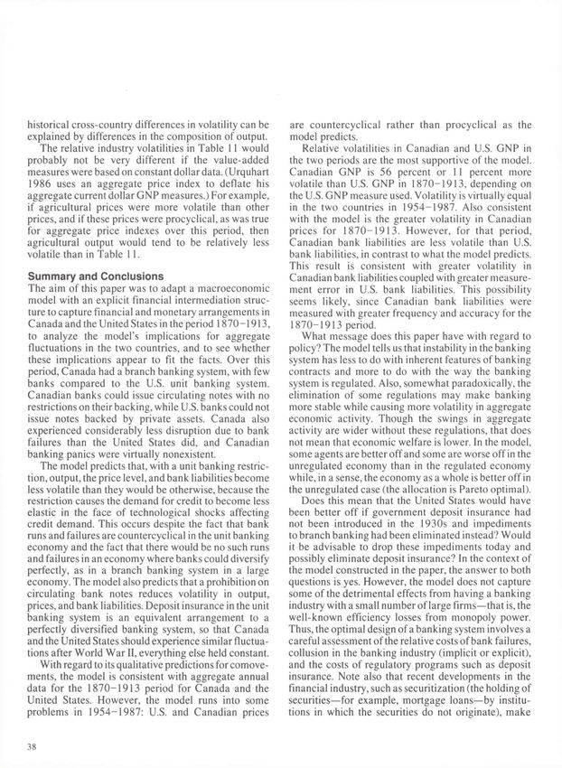
37historical cross-country differences in volatility can be are countercyclical rather than procyclical as the
explained by differences in the composition of output. model predicts.
The relative industry volatilities in Table 11 would Relative volatilities in Canadian and U.S. GNP in
probably not be very different if the value-added the two periods are the most supportive of the model.
measures were based on constant dollar data. (Urquhart Canadian GNP is 56 percent or 11 percent more
1986 uses an aggregate price index to deflate his volatile than U.S. GNP in 1870-1913, depending on
aggregate current dollar GNP measures.) For example, the U.S. GNP measure used. Volatility is virtually equal
if agricultural prices were more volatile than other in the two countries in 1954-1987. Also consistent
prices, and if these prices were procyclical, as was true with the model is the greater volatility in Canadian
for aggregate price indexes over this period, then prices for 1870-1913. However, for that period,
agricultural output would tend to be relatively less Canadian bank liabilities are less volatile than U.S.
volatile than in Table 11. bank liabilities, in contrast to what the model predicts.
This result is consistent with greater volatility in
Summary and Conclusions Canadian bank liabilities coupled with greater measure-
The aim of this paper was to adapt a macroeconomic ment error in U.S. bank liabilities. This possibility
model with an explicit financial intermediation struc- seems likely, since Canadian bank liabilities were
ture to capture financial and monetary arrangements in measured with greater frequency and accuracy for the
Canada and the United States in the period 1870-1913, 1870-1913 period.
to analyze the model's implications for aggregate What message does this paper have with regard to
fluctuations in the two countries, and to see whether policy? The model tells us that instability in the banking
these implications appear to fit the facts. Over this system has less to do with inherent features of banking
period, Canada had a branch banking system, with few contracts and more to do with the way the banking
banks compared to the U.S. unit banking system. system is regulated. Also, somewhat paradoxically, the
Canadian banks could issue circulating notes with no elimination of some regulations may make banking
restrictions on their backing, while U.S. banks could not more stable while causing more volatility in aggregate
issue notes backed by private assets. Canada also economic activity. Though the swings in aggregate
experienced considerably less disruption due to bank activity are wider without these regulations, that does
failures than the United States did, and Canadian not mean that economic welfare is lower. In the model,
banking panics were virtually nonexistent. some agents are better off and some are worse off in the
The model predicts that, with a unit banking restric- unregulated economy than in the regulated economy
tion, output, the price level, and bank liabilities become while, in a sense, the economy as a whole is better off in
less volatile than they would be otherwise, because the the unregulated case (the allocation is Pareto optimal).
restriction causes the demand for credit to become less Does this mean that the United States would have
elastic in the face of technological shocks affecting been better off if government deposit insurance had
credit demand. This occurs despite the fact that bank not been introduced in the 1930s and impediments
runs and failures are countercyclical in the unit banking to branch banking had been eliminated instead? Would
economy and the fact that there would be no such runs it be advisable to drop these impediments today and
and failures in an economy where banks could diversify possibly eliminate deposit insurance? In the context of
perfectly, as in a branch banking system in a large the model constructed in the paper, the answer to both
economy. The model also predicts that a prohibition on questions is yes. However, the model does not capture
circulating bank notes reduces volatility in output, some of the detrimental effects from having a banking
prices, and bank liabilities. Deposit insurance in the unit industry with a small number of large firms—that is, the
banking system is an equivalent arrangement to a well-known efficiency losses from monopoly power.
perfectly diversified banking system, so that Canada Thus, the optimal design of a banking system involves a
and the United States should experience similar fluctua- careful assessment of the relative costs of bank failures,
tions after World War II, everything else held constant. collusion in the banking industry (implicit or explicit),
With regard to its qualitative predictions for comove- and the costs of regulatory programs such as deposit
ments, the model is consistent with aggregate annual insurance. Note also that recent developments in the
data for the 1870-1913 period for Canada and the financial industry, such as securitization (the holding of
United States. However, the model runs into some securities—for example, mortgage loans—by institu-
problems in 1954-1987: U.S. and Canadian prices tions in which the securities do not originate), make
38You can also read