An Attention-Based Deep Sequential GRU Model for Sensor Drift Compensation
←
→
Page content transcription
If your browser does not render page correctly, please read the page content below
7908 IEEE SENSORS JOURNAL, VOL. 21, NO. 6, MARCH 15, 2021
An Attention-Based Deep Sequential GRU
Model for Sensor Drift Compensation
Tanaya Chaudhuri , Min Wu , Senior Member, IEEE, Yu Zhang,
Pan Liu, and Xiaoli Li , Senior Member, IEEE
Abstract —Sensor accuracy is vital for the reliability of
sensing applications. However, sensor drift is a common
problem that leads to inaccurate measurement readings.
Owing to aging and environmental variation, chemical gas
sensors in particular are quite susceptible to drift with time.
Existing solutions may not address the temporal complex
aspect of drift, which a sequential deep learning approach
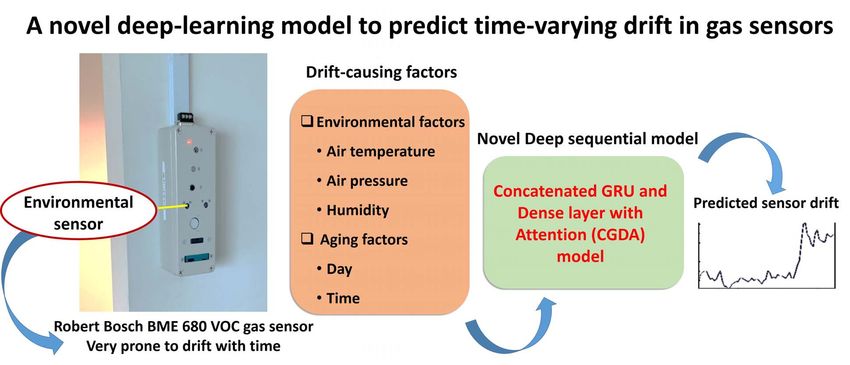
could capture. This article proposes a novel deep sequential
model named Concatenated GRU & Dense layer with Atten-
tion (CGDA) for drift compensation in low-cost gas sensors.
Concatenation of a stacked GRU (Gated Recurrent Unit) block
and a dense layer is integrated with an attention network, that
accurately predicts the hourly drift sequence for an entire day.
The stacked GRU extracts useful temporal features layer by layer capturing the time dependencies at a low computational
expense, while the dense layer helps in retention of handcrafted feature knowledge, and the attention mechanism
facilitates adequate weight assignment and elaborate information mapping. The CGDA model achieves a significant
mean accuracy over 93%, outperforming several state-of-the-art shallow and deep learning models besides its ablated
variants. It can greatly enhance the reliability of sensors in real-world applications.
Index Terms — Attention network, deep learning, drift compensation, gas sensor drift, gated recurrent unit.
I. I NTRODUCTION (3) adaptive approaches [4], [5]. Univariate approaches
comprise sensor signal processing such as baseline manip-
G AS sensors are substantially significant given their wide-
spread applications ranging from environmental moni-
toring to air quality and pollution checks, biometrics, food and
ulation, frequency domain filtering, multiplicative correc-
tion or estimation theory [6]–[8]. These are simplified methods
agriculture, medical diagnosis and robotics. However, chemi- where compensation is applied to each sensor independently.
cal changes by aging and environmental variation commonly Their drawbacks are that firstly, they may not be adequate
lead to sensor drift with the passage of time. This results in when the drift is complex in nature which is often the real
inaccurate measurement readings and deterioration of sensor case, and secondly, they are sensitive to sample rate changes.
reliability [1]. Low-cost metal-oxide gas sensors in particular Multivariate approaches comprise cluster analysis such as
are attractive owing to their cost-effectiveness, operational ease self-organizing maps [9], signal correction and deflation by
and spatial coverage, but they get problematic with time by dimension reduction methods [10], or system identification
their susceptibility to drift [2], [3]. Although several methods methods [11]. Their drawbacks are that firstly, they need
have been developed over the past decades, drift compensation frequent sampling and secondly, these approaches may not
still remains a challenge. accurately separate the undesired component from the useful
Drift compensation approaches can be categorised as components in the case of complex drift effect with noise [12].
(1) univariate approaches, (2) multivariate approaches and On the other hand, the adaptive approaches comprise
machine learning algorithms. These approaches are popular
Manuscript received October 9, 2020; revised December 5, 2020; because they allow the flexibility to add non-linear relation-
accepted December 6, 2020. Date of publication December 14, 2020; ships in the drift model, without making any prior assumptions
date of current version February 17, 2021. This work was supported of the drift signal. Some of the related works on machine
by the Agency for Science, Technology and Research (A*STAR) under
the Republic of Singapore’s Research Innovation Enterprise (RIE2020) learning based drift correction are discussed in the next
Advanced Manufacturing and Engineering Industry Alignment Fund - section.
Pre-Positioning Programme (IAF-PP) under Grant A1789a0024. The
associate editor coordinating the review of this article and approving it
for publication was Dr. Irene Taurino. (Corresponding author: Min Wu.)
The authors are with the Institute for Infocomm Research (I2R), A. Related Works on Adaptive Approaches
A*STAR, Singapore 138632 (e-mail: tanaya_chaudhuri@i2r.a- An electronic-nose (e-nose) in the machine olfaction sys-
star.edu.sg; wumin@i2r.a-star.edu.sg; zhang_yu@i2r.a-star.edu.sg;
liu_pan@i2r.a-star.edu.sg; xlli@i2r.a-star.edu.sg). tem serves the purpose of odor recognition and has wide
Digital Object Identifier 10.1109/JSEN.2020.3044388 applications. However, drift in the gas sensors affects their
1558-1748 © 2020 IEEE. Personal use is permitted, but republication/redistribution requires IEEE permission.
See https://www.ieee.org/publications/rights/index.html for more information.
Authorized licensed use limited to: Nanyang Technological University. Downloaded on May 12,2021 at 10:09:58 UTC from IEEE Xplore. Restrictions apply.
CHAUDHURI et al.: ATTENTION-BASED DEEP SEQUENTIAL GRU MODEL FOR SENSOR DRIFT COMPENSATION                                                                  7909

measurements and thereby hampers the reliability of the e-nose                 pattern [12]. Very few studies such as [26] have considered
predictions. Marco et. al provides an excellent review of the                  this aspect and explored the time-series prediction of drift
machine learning pattern recognition methods used for gas dis-                 signal. In this study [26], Zhang et. al developed a drift
crimination in sensor arrays [4]. Many of these methods seek                   prediction model using chaotic time series prediction method
to overcome the time-dependent drift while classifying gases.                  based on phase space reconstruction (PSR) and single-layered
In this respect, Support Vector Machine (SVM) classifiers have                 neural networks (SNN). Mumyakmaz et. al [27] employed
been widely used [13], [14]. Vergara et. al used a weighted                    two neural networks with the first as a classifier to identify
combination of SVMs trained at different points of time which                  the gases, and the second to predict the concentration ratios
helped to counteract the drift [13]. Verma et. al [14] added reg-              of the gases in a sensor array. De Vito et. al [28] applied time
ularization to this weighted ensemble which further improved                   delay support vector regressor (SVR) and time delay neural
accuracy and reduced over-fitting as well. Rehman et. al [15]                  network to predict the real-time gas concentrations in sensor
proposed heuristic Random Forest (RF) to classify gases where                  array. However, the sensor drift was not studied in both these
RF learning was embedded with particle swarm optimization                      works.
to compensate the drift. Brahim et. al [16] adopted Gaussian
Mixture Models (GMM) to develop a gas classifier which                         B. Contributions of This Paper
counteracts the drift by extracting robust features using a                       Although a great many excellent works have been done
simulated drift.                                                               on adaptive approaches to compensate drift, there are a
   Recently, deep learning has been explored for gas recogni-                  few concerns. Firstly, most of the existing machine learning
tion with drift suppression. Tian et. al [17] designed a gaussian              approaches are pattern recognition algorithms aimed at clas-
Deep Belief Network (DBN) to identify gases under sensor                       sification of gases in sensor arrays. Very few studies have
drift. It used the DBN as a non-linear function to learn the                   explored direct prediction of the drift values. In this study,
drift based differences between the source and target domains.                 we aim at building a model focused on the prediction of
Liu et. al [18] adopted DBN and stacked sparse autoencoder                     sensor drift. The predicted drift can be used to correct sensor
(sSAE) to extract deep features, and these features were later                 readings, which can make applications like gas recognition
used to train a gas classifier that could reduce the drift.                    more reliable.
Luo et. al [19] adopted DBN to extract depth characteristics                      Secondly, the parameters that cause sensor drift have rarely
of the drifted gas sensor data. Then, the DBN model was                        been incorporated in the classification or prediction mod-
coupled with an SVM which improved gas recognition under                       els. Based on the causes, sensor drift is categorised into
drift. Altogether, several such drift correcting machine learning              two types: (a) The ‘first-order’ or ‘real’ drift, results from
classifiers have progressed the odor recognition arena over the                sensitivity changes in chemical sensors due to aging and
last decade.                                                                   poisoning. It often occurs over long periods of time. (b) The
   The drifted data has a different projected distribution than                ‘second-order’ drift, may result from the slow changes in the
the clean data. Capturing this difference helps to separate                    external environment such as ambient temperature, pressure
the two types of data and reduce the drift through subspace                    etc. It may occur over short time periods, but the fluctuations
learning. Zhang et. al [20] proposed an unsupervised subspace                  can significantly alter sensor response [1], [6], [9], [13].
projection approach that reduced the drift by projecting the                   Moreover, practically it is extremely difficult to empirically
data onto a new common subspace using principal component                      differentiate between these two drifts [13]. In this study,
analysis (PCA). Such projection approaches were extended to                    we incorporate these aging and environmental drift-causing
transfer learning based feature adaptation in [21]. The drift                  factors into the feature space of our drift prediction model.
was compensated by aligning the principal component sub-                          Thirdly, most of the current machine learning based drift
space between the clean and the drifted data. Similarly, these                 solutions are shallow learning methods. The few methods that
subspace learning capabilities were extended to cross-domain                   have explored deep learning are focused on gas classification
discriminative learning in [22]. Odor recognition models could                 as well. Deep learning has definitive power to capture the
be transferred between different e-noses using this method.                    complexities in data and therefore would be more suitable for
Such dimensionality reduction methods are often incorporated                   handling complex drift signals. Furthermore, given the ‘tempo-
as a pre-processing technique in gas classifiers.                              ral’ nature of ‘time’-varying drift, sequential neural networks
   In this respect, several transfer learning based domain adap-               such as the Gated Recurrent Unit (GRU) network [29] could
tation methods have been proposed. Yan et. al [23] proposed                    be apt for modelling the drift. Several advantages of the GRU
a drift-correcting autoencoder using transfer learning while                   such as the ability to capture time dependencies, temporal
Zhang et. al [24] proposed domain-adaptation Extreme Learn-                    feature learning and low computational cost make it suitable
ing Machines (ELM) to suppress drift. Liu et. al proposed a                    for modelling the drift in our study. However, modelling longer
semi-supervised domain adaption method to compensate drift                     sequences can suffer from information loss. The attention
using a weighted geodesic flow kernel (GFK) and a classifier                   mechanism [30] can prevent such loss, besides providing
with manifold regularization [25].                                             better interpretability and appropriate information mapping.
   In most of these adaptive methods, it is assumed that the                   Attention mechanism is a recent revolutionary concept in deep
drift trend can be traced through its direction in projected                   learning. It selectively pays ‘attention’ to the most relevant
subspace or its distribution. However, long-term drift do                      information in deep neural networks while ignoring the non-
not always have a consistent direction trend or a regular                      relevant parts, by assigning appropriate weights. It can help

   Authorized licensed use limited to: Nanyang Technological University. Downloaded on May 12,2021 at 10:09:58 UTC from IEEE Xplore. Restrictions apply.
7910                                                                                                IEEE SENSORS JOURNAL, VOL. 21, NO. 6, MARCH 15, 2021

Fig. 1. Architecture of the proposed CGDA model for drift prediction. Here, fCGDA : the overall CGDA model, X: the CGDA model input, : the
CGDA model drift output, nd : the number of days (batch size), nf : the number of input features, and ‘24’ represents the number of hours in a day.
Enclosed dotted portion illustrates a single day (sample) for simplicity purpose, where fg : the GRU network, fd1 : the first dense network, fa : the
attention network, and fd2 : the second dense network. X , X d 1 , X a , X d 2 are the inputs and Y g , Y d 1 , Y a ,  are the outputs of fg , fd1 , fa and fd2
networks, respectively.

our model focus on the most relevant hidden states of the                             The rest of the paper is organized as follows: Section II
input sequences for drift prediction.                                              introduces the proposed CGDA model’s framework.
   In this article, we propose a deep learning based sequential                    Section III describes the experimental settings and the
model for drift compensation in low cost gas sensors, incorpo-                     sensor dataset followed by the results and discussions in
rating the aging and environmental drift-causing factors. The                      section IV. Finally, section V highlights the concluding
specific contributions are:                                                        remarks and future work.
   • We propose a novel deep sequential model termed as
     the Concatenated GRU and Dense layer with Attention                                        II. P ROPOSED CGDA M ODEL
     (CGDA) model for drift compensation in low-cost gas                            This section describes the framework of the Concatenated
     sensors. Concatenation of a stacked GRU block and a                           GRU and Dense layer with Attention (CGDA) model.
     dense layer is integrated with attention mechanism, that
     accurately predicts the drift sequence for an entire day.
                                                                                   A. Overall Framework
   • The stacked GRU block extracts useful temporal features
     layer by layer capturing time dependencies at a low com-                         The architecture of the proposed CGDA model is illustrated
     putational expense, which enhances the drift prediction.                      in Fig. 1. Broadly, the CGDA model fC G D A comprises a GRU
   • The dense layer helps in better retention of feature
                                                                                   block that is concatenated with a dense layer, and followed by
     information by supporting handcrafted features, while the                     an attention network.
     attention network facilitates adequate weight assignment                         The input feature space comprises of a batch of data over
     and prevents information loss along the input sequence;                       n d number of days. Each day is a sample in the data. Each
     this aids in appropriate representation of the drift and                      sample (day) consists of a time-series sequence of n f different
     further enhances its prediction.                                              features. The length of each sequence is 24, considering there
   • Intensive feature extraction by the GRU and dense lay-
                                                                                   are 24 hourly points in a day corresponding to time-slots
     ers, and elaborate information mapping by the attention                       1, 2, .. 24. Considering n d = number of days in the data
     network improve the model’s drift prediction ability. It’s                    (batch size) and n f = number of features, the input feature
     efficacy is validated through a comprehensive chronolog-                      tensor set X ∈ Rnd ×n f ×24 is denoted as:
                                                                                                       1,2,..n
     ical comparison with 8 different state-of-the-art shallow                                      X 1,2,..ndf [t] where t = {1, 2, ..24}
     and deep learning models including an ablation study.
   • The input feature space addresses the environmental and                       We consider the target drift  ∈ Rnd ×24 as a time sequence
     aging factors of drift. The study findings are corroborated                   of hourly drift values along a day which is denoted as:
     through an experimental dataset generated by our institute
                                                                                            k = {δ1k , δ2k , . . . δ24
                                                                                                                     k
                                                                                                                        }, where k = {1, 2, ..n d }
     by deploying a robust sensor-network that collected data
     over 4 to 14 months duration at indoor and semi-indoor                        The CGDA model can be symbolically represented as f C G D A :
     locations within office premises.                                             X → .

       Authorized licensed use limited to: Nanyang Technological University. Downloaded on May 12,2021 at 10:09:58 UTC from IEEE Xplore. Restrictions apply.
CHAUDHURI et al.: ATTENTION-BASED DEEP SEQUENTIAL GRU MODEL FOR SENSOR DRIFT COMPENSATION                                                                   7911

B. GRU Block                                                                    C is concatenated with the output generated from the previous
   The feature input tensor is fed to the GRU network f g .                     time step. The process repeats for all time steps. Finally, this
Note that the GRU may be single or multi-layered (stacked)                      is followed by a second dense layer network f d2 also with
depending upon hyperparameter optimization. For a given                         ReLu as the activation function (similarly using equations 5-6),
time-step t, the input is X[t] ∈ Rnd ×h and the computations                    to map the attention layer output Y a to the target drift
are:                                                                            sequence . The CGDA model f C G D A : X →  can thus be
                                                                              summarized as:
 R[t] = σ X[t]W xr + H[t − 1]W hr + br                   (1)
                                                                                                    GRU f g     :   X → Yg                                 (8)
  Z[t] = σ X[t]W x z + H[t − 1]W hz + bz                 (2)
                                                                                                 Dense1 f d1    :   X d1 → Yd1                             (9)
 H̃[t] = tanh X[t]W zh + (R[t]  H[t − 1])W hh + bh      (3)                                      Attention f a   :   X a (Y g , Yd1) → Ya                  (10)

 H[t] = Z[t]  H[t − 1] + 1 − Z[t]  H[t] ˜              (4)                                       Dense2 fd2     :   X d2 (Ya ) →                         (11)

where, H[t − 1] ∈ Rnd ×h is the hidden state of the last                          The equations of all activation functions used in the model
time-step, R[t] ∈ Rnd ×h is the reset gate, Z[t] ∈ Rnd ×h is                    are summarized below:
the update gate, W xr , W x z ∈ Rnd ×h and W hr , W hz ∈ Rh×h                                    σ (x) =
                                                                                                                1
                                                                                                                                              (12)
are weight parameters, br , bz , bh ∈ R1×h are the biases, and                                            (1 + e−x )
h is the number of features in the layer (h = n f for first                                               (e x − e−x )
                                                                                              tanh(x) = x                                     (13)
layer). H̃[t] is the candidate hidden state and H[t] is the new                                            e + e−x
state. σ denotes sigmoid function and  denotes Hadamard                                   ReLU (x) = max(x, 0)                               (14)
                                                                                                               e xi
product. In case of a multi-layered GRU network, the input                                          x ) = m
                                                                                       so f tmax i (                x j for i = 1, . . . , m (15)
of a particular layer is the hidden state H[t] of the previous                                                j =1 e
layer. No dropout has been used between the layers.
                                                                                E. Rationale Behind Model Structure
C. Concatenation With Dense Layer                                                  The advantages of the GRU are manifold. First, its suitabil-
                                                                                ity for sequence modelling is apt for our time-varying drift
   Simultaneously, the feature tensor is reshaped to
                                                                                which is a time-series data. Secondly, its ability to capture
X d1 ∈ Rnd ×(n f ∗24 ) vector which is fed to a single dense
                                                                                time dependencies is apt for our fixed-length drift sequences.
layer network f d1 . Rectified Linear Unit (ReLU) is used as
                                                                                The reset gate and the update gate help capture the short-
the activation function. Assuming that (X d1 )k is the input
                                                                                term and long-term dependencies, respectively. Moreover,
vector and (Yd1)k is the output vector for the k t h training
                                                                                the GRU extracts important temporal features layer-by-layer
sample, the dense layer can be formulated as:
                                                                             that improves model robustness. Additionally, a GRU unit has
                  k                            k                                few parameters leading to faster training which is an important
              Vi = ReLU             wi j (x d1) j − bh i   (5)
                                                                                requirement for the stacked layers in our model. The dense
                                                                               layer helps in better retention of the feature information. While
           (Yd1 )kp =     Vik w pi − bo p                  (6)
                                                                                the GRU generates deep features, the dense layer retains the
where, Vik is the output of hidden neuron i , wi j is weight                    handcrafted features. The placement of the attention network
parameter from input layer neuron j to hidden layer neuron i ,                  in the CGDA model has multiple benefits:
bh i is the bias of hidden neuron i , w pi is the weight parameter                 • Without the attention layer, equal weights would be
from hidden neuron i to output neuron p, and bo p is the bias                         assigned to all the states in the concatenated output from
of output neuron p. The output Y g from the last layer of GRU                         the GRU and the dense layer. With attention network,
and the output Yd1 from the dense layer are concatenated.                             we have weighted attention to the states i.e., assigning
                                                                                      adequate weightage to each state in the concatenated
                                                                                      output. It also allows us to better interpret the contribution
D. Attention Mechanism                                                                of the two participating models i.e. GRU vs. Dense1.
   The concatenated layer X a (Y g , Yd1) is fed to an attention                   • It gives attention to the entire input sequence instead
network f a . Soft attention is used. The attention mechanism                         of just the last state. This prevents information loss for
is explained below.                                                                   long input sequences unlike a seq2seq network where
   Firstly, the input concatenated sequence is encoded into                           information tends to get lost towards the end.
a set of internal states h 1 , h 2 , . . . h m . Alignment scores are              • For each time step, a separate context vector is computed
calculated for each encoded state by training a feedforward                           by computing the attention weights. Thus, through this
network that learns to recognize relevant states by creating                          mechanism, our model can discover interesting mappings
higher scores for states that deserve attention, and vice-versa.                      between various segments of the input sequence and their
Attention weights α1 , α2 , ..αm are generated by applying soft-                      corresponding parts in the output sequence.
max function to the scores. Note that the attention weight
vector gives a probabilistic interpretation i.e. α ∈ [0, 1] and
                                                                               F. Feature Space
   α = 1. Next, the context vector is computed:
                                                                                   A 3-stage approach is used for feature refinement: firstly,
            C = α1 ∗ h 1 + α2 ∗ h 2 + . . . + αm ∗ h m                   (7)    the initial feature space is selected based on domain knowledge

    Authorized licensed use limited to: Nanyang Technological University. Downloaded on May 12,2021 at 10:09:58 UTC from IEEE Xplore. Restrictions apply.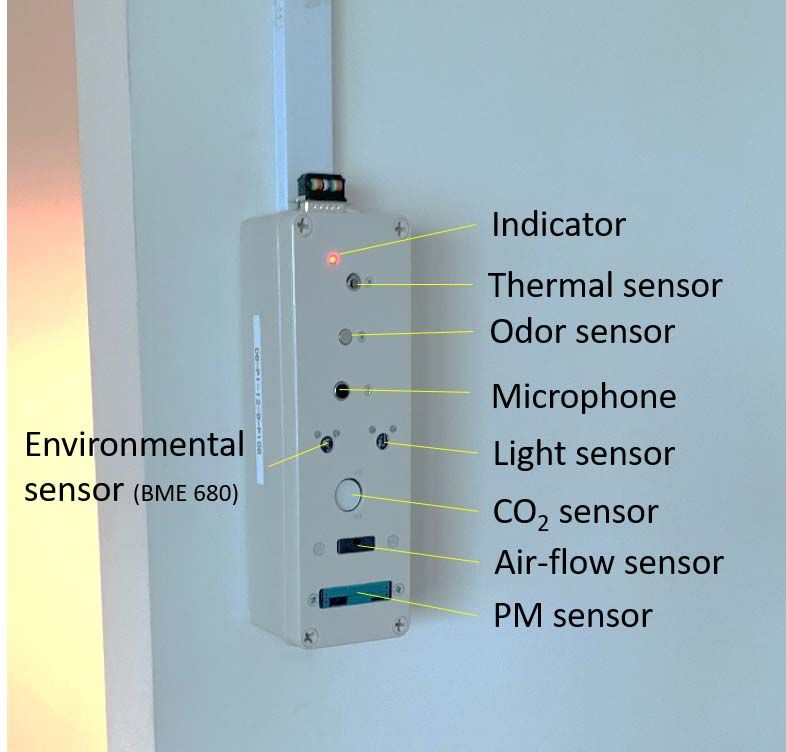
7912                                                                                                IEEE SENSORS JOURNAL, VOL. 21, NO. 6, MARCH 15, 2021

of drift-causing factors; secondly, filter method is used to
statistically evaluate the relevant subset, and lastly, intrinsic
method is used by the deep layers of the CGDA model. The
following parameters are selected for the initial feature set,
that addresses the factors causing drift:
   • Environmental factors: air temperature (Ta ), air pressure
      (Pa ), relative humidity (R H ), particulate matter (P M2.5 )
   • Aging factors: elapsed days (elap-day), hourly time-slot
      in the day (time-slot)
   The elap-day feature denotes the number of days elapsed
since the sensor deployment. Note that elap-day is not the
same as the sample number; there may be missing samples                                 Fig. 2. A labelled sensor node deployed at measurement site.
in the data. In Fig. 1, the days 1 to n d are samples, each
containing elap-day as a feature. The time-slot feature denotes
the time-slot among the 24 hours in a day. While the aging                         several state-of-the-art machine learning methods. Shallow
effect is predominantly represented by elap-day, the time-slot                     models namely, decision tree regression (DTR) [31], support
can represent the daily cyclic influence.                                          vector regression (SVR) [32], and random forest (RF) [15]
   Thereafter, a filter method namely a simple Pearson                             are implemented besides the SNN. Deep models namely, long
Product-Moment correlation analysis is performed to eval-                          short-term memory (LSTM) [33] and 1D convolutional neural
uate the linear relationships. A confidence interval of 90%                        network (CNN) [34] are employed besides the deep ablated
( p < 0.1) is used for the significance tests. Finally, an intrin-                 variants (GRU, CGD). LSTM is a popular gated sequential
sic method performs automatic feature selection during the                         network, and 1D-CNN is suitable for time-series regression
model’s training process, which in this case is facilitated by                     with sensor data. Therefore, 4 shallow models (DTR, SVR,
the deep layers of the CGDA model.                                                 RF, SNN) and 4 deep models (LSTM, CNN, GRU, CGD) are
                                                                                   implemented besides CGDA for the comparative analysis.
          III. E XPERIMENTAL S ETTINGS AND DATA                                       It is to be noted that although both GRU and LSTM
A. Experimental Settings                                                           keep long-term dependencies while handling the exploding/
   1) Hyperparameter Optimization: For each experiment,                            vanishing gradient problems, GRU does not require mem-
a hyperparameter optimization is performed to select the best                      ory units unlike LSTM. Since our input sequence length is
model during training. The ranges covered are- learning rate:                      fixed (24 time-steps), GRU is a better choice compared to
[10−6 , 10−4 ], recurrent layers in the GRU block: [1, 5],                         LSTM whose benefits weigh up mainly for longer sequences.
hidden GRU units in a layer: [12, 400], hidden neurons in                          Moreover, GRU uses less training parameters thereby having
the dense layer: [12, 200]. For each experiment, the number of                     lower computational cost and faster response. Therefore, we do
neurons in the output layer of GRU (Yg ) and Dense1 (Yd1 ) are                     not compare a model with LSTM in place of GRU.
kept equal before concatenation. Early-stopping regularization
based on the validation error is used, with train:validation size                  B. Sensor Data Collection
ratio set at 80:20, and the number of epochs limited to 50,000.                       Several sensors namely, an environmental sensor, a par-
The Adam optimizer is implemented and the loss function of                         ticulate matter sensor, an air-flow sensor, a CO2 sensor,
the model is set as root-mean-squared-error (RMSE).                                an ambient light sensor, an odor sensor, a thermal sensor and
   2) Performance Metric: We evaluate the model’s perfor-                          a microphone, are embedded together using a TI AM335x
mance using the drift-prediction-accuracy (DPA) based on the                       BeagleBone Black Robotics Cape, and encased into a compact
mean-absolute-percentage-error (MAPE):                                             box referred to as a ‘sensor node’ or simply ‘node’ as
                                                                                 labelled in Fig. 2. The sensor models are listed in Table I.
                           1   δi − δˆi
                              N
               M AP E =                                    (16)                  The BME680 environmental sensor is a widely used low-
                          N      δi                                              cost MOX based gas sensor meant for monitoring volatile
                                    i=1
                    D P A = (1 − M A P E) × 100 (%)                       (17)     organic compounds (VOC). It measures three environmental
                                                                                   parameters namely, air temperature, air pressure and humidity.
where, δi and δˆi are the true and the predicted drifts, respec-                   Freshly manufactured new BME680 sensors are cased. A node
tively, and N is the number of samples.                                            continuously senses the environment, performs edge process-
   3) Ablation Study: An ablation study is important for under-                    ing, and sends the analysed data to a backend server where it
standing the causality in the model. The ablated variants                          is stored and viewed real-time through a web portal.
of the CGDA model are implemented which are, GRU                                      Several sensor nodes were deployed within the office
(a single/stacked GRU model) [29], SNN (a single-layered                           premises of the Institute for Infocomm Research, ASTAR,
neural network model) [26] and CGD (concatenated GRU                               Singapore, for collection of long-time drift performance as
block and dense layer model without an attention mechanism).                       described in Table II. Nodes A and B were placed in indoor
   4) Comparison With State-of-the-Art: To comprehensively                         locations, while nodes C and D were deployed in semi-indoor
evaluate our proposed CGDA model, we compare against                               locations. The indoor locations are rooms in the interior of

       Authorized licensed use limited to: Nanyang Technological University. Downloaded on May 12,2021 at 10:09:58 UTC from IEEE Xplore. Restrictions apply.
CHAUDHURI et al.: ATTENTION-BASED DEEP SEQUENTIAL GRU MODEL FOR SENSOR DRIFT COMPENSATION                                                                  7913

                                                                    TABLE I
                                               S UMMARY OF THE E NCASED S ENSORS W ITHIN A N ODE

                           TABLE II
 D EPLOYMENT L OCATIONS AND D URATIONS OF THE S ENSOR N ODES
        U SED FOR C OLLECTION OF D RIFT P ERFORMANCE

building with no access to outdoors, while the semi-indoor
locations have an enclosed boundary with direct access to the
outdoors. The data collection duration spanned 4 to 14 months.
   Multiplicative drift is used in this study and is denoted
by δ (unitless) as the ratio between the current (drifted state)
resistance to the actual (non-drifted state) resistance response.
Similar to previous works [13], [35], [36], the multiplicative
drift is based on the assumption that the sensors are calibrated
before being deployed and therefore the response during the
initial period post deployment can be considered drift-free.
The data was logged at intervals of 3 seconds. For this study,
we averaged the data per hour. Besides the hourly drift,
the hourly mean of features air temperature, pressure, relative
humidity, and PM2.5 were computed. Note that air-flow is
removed from consideration as a feature, due to its almost con-
stant value. The CO2 , light intensity, odor and thermal sensors,
and the microphone were meant for monitoring purposes only.

C. PCA for Time-Varying Drift Illustration
   Principal component analysis (PCA) is used to inspect the
drift across the months as shown in Fig. 3a. PCA is applied
to project the samples to a 2-D subspace, where each day is
a sample consisting of 24 timeslot (hourly) drifts. The plots
depict the first two principal components (PC) and the first
component PC1 accounts for the majority of variance in the
drift: 0.957 (node A), 0.806 (node B), 0.958 (node C) and
0.839 (node D). For simplicity, only the first three months                    Fig. 3. (a) Illustration of the drift across months M1 to M3. (b) Sensor
                                                                               response along first 4 months M1-M4.
are analysed. Firstly, it is evident from the visual inspec-
tion that there is an obvious drift with time across months,
which are separable while sliding horizontally along PC1.                            IV. E XPERIMENTAL R ESULTS AND D ISCUSSIONS
Secondly, different data distributions among the nodes indicate                A. Feature Significance by Filter Method
that the drift varies from one sensor to another. For visual                      The results of the Pearson correlation and the significance
clarity, the sensor response (VOC resistance) of only the first                tests between the sensor drift and the features are summa-
4 months are illustrated in Figure 3b. The scale of response                   rized in Fig. 4. Here, hs, ls, and ns denote high significance
varies between the four nodes as they are placed in different                  ( p < 0.05), low significance ( p < 0.1), and no significance
environments. Therefore, it is vital to develop separate drift                 ( p ≥ 0.1), respectively. Most features reveal significant
model for each node. While the basic model architecture may                    correlation with the sensor drift. Aging as the major cause
be same, the hyperparameters have been tuned per node for                      of first-order drift is validated by the highest correlations with
best performance.                                                              elap-day. All features show significance except for R H in

   Authorized licensed use limited to: Nanyang Technological University. Downloaded on May 12,2021 at 10:09:58 UTC from IEEE Xplore. Restrictions apply.
7914                                                                                                IEEE SENSORS JOURNAL, VOL. 21, NO. 6, MARCH 15, 2021

                                                                                                                TABLE III
                                                                                       C HRONOLOGICAL C OMPARISON OF MAPE (%) A MONG VARIOUS
                                                                                        M ODELS . B EST P ERFORMANCES A RE H IGHLIGHTED IN B OLD

Fig. 4. Significance of Pearson correlation between the sensor drift and
the initial features. hs = high significance (p < 0.05), ls = low significance
(p < 0.1), ns = no significance (p ≥ 0.1).

node C and time-slot in node D, which could be attributed to
the comparatively smaller sample sizes. Interestingly, the sig-
nificance of time-slot feature supports our speculation that the
time of the day can have some catalytic effect on the drift.
The movements and the occupancy in office spaces usually
tend to have a daily as well as a weekly pattern, which
the combination of elap-day and time-slot may represent.
The collective effect of these factors have complex non-
linearities that the non-linear CGDA as an intrinsic method
can adequately model.

B. Drift Prediction Performance
   The chronological drift prediction performance of all the
models are presented in Table III and Fig. 5. Table III lists the
test MAPE values and Fig. 5 graphically summarizes the DPA
values. The first column in Table III depict the test month.
Note that the table lists the test error; a model trained on the
first month (M1) is tested on the second month (M2), next a
model trained on the first two months (M1-2) is tested on the
third month (M3) and so on.
   It is observed from Table III that the proposed CGDA
model achieves the best performance consistently across most
of the chronological experiments. It exhibits mean MAPE
of 5.5% to 7.59% only, as compared to much larger errors
in the traditional shallow models. It predicts the drift in
sensor nodes A, B, C and D with excellent mean accuracies
of 94.50%, 93.66%, 92.41% and 92.58%, respectively. As seen
for node A in Fig. 5, DTR, SVR, and RF perform poorly due
to low training data in the first experiment (M2). However,
CGDA performs well even with just one month training data.
From Fig. 5, it is further evident that the CGDA model
consistently achieves high DPA (above 90%) across most
months. This is a remarkable advantage of the CGDA model
in terms of reliability, as compared to the remaining models.
   As for ablation study, GRU is better able to predict the
drift as compared to SNN. The integration of the GRU layers                               Fig. 5. Comparison of the chronological DPA of all models.
with a dense layer in CGD further enhances its ability to
formulate the drift. While the dense layer uses the supplied
handcrafted features, the deep GRU layers generate important                       relevant and adequate information, which further enhances the
temporal features. The addition of the attention layer to                          ability to capture the drift.
this concatenated integration helps to compute the weights                            The results are further categorised based on the type of
appropriately, thereby preventing loss of information. This                        the sensor location: indoor vs. semi-indoor, and the type
weight assignment in CGDA allows extracting only the most                          of the learning model: deep learning vs. shallow learning.

       Authorized licensed use limited to: Nanyang Technological University. Downloaded on May 12,2021 at 10:09:58 UTC from IEEE Xplore. Restrictions apply.
CHAUDHURI et al.: ATTENTION-BASED DEEP SEQUENTIAL GRU MODEL FOR SENSOR DRIFT COMPENSATION 7915
TABLE IV The plot in Fig. 6 reveals that the Y g weights cover a much
S UMMARY OF C ATEGORICAL M EAN DPA (%) wider range with greater probability of larger values, while the
Yd1 weights are limited with probability of smaller values. The
larger weights for GRU indicate that the GRU block makes
a greater contribution as compared to Dense1. It denotes that
the deep features created by the GRU have more significance
than the handcrafted features fed to the dense layer.
V. C ONCLUSION
In this article, we proposed a novel deep-sequential model
termed as the CGDA model for drift compensation in low-
cost gas sensors. Concatenation of a stacked GRU block and
a dense layer is integrated with attention mechanism, that
predicts the drift sequence for an entire day, through intensive
feature extraction and elaborate information mapping. The
stacked GRU layers extract useful deep temporal features
layer by layer capturing time dependencies at a low com-
putational expense, the dense layer helps retain handcrafted
feature information, while the attention network facilitates
adequate weightage assignment and prevents information loss.
In addition, the feature space addresses the environmental and
aging effects on the sensor. The efficacy of the CGDA model
is validated through its superior performance with over 93%
mean DPA as compared to 8 state-of-the-art shallow and deep
learning models across multiple nodes at varied locations.
Fig. 6. Split-violin plot of the attention weights. The CGDA model can help realize remote sensor calibration
and greatly enhance the reliability of gas sensors in real-world
applications. Its utility can be extended to other sensors as
Table IV summarizes the mean DPAs for this categorical well through appropriate improvisations such as a suitable
analysis. CGDA achieves an overall mean DPA of 93.29% feature-space. In future, we plan to address the issue of noisy
across all nodes, outperforming the rest while DTR attains the data [37] for sensor drift prediction. We will also continue
least mean DPA at 72.85%. Firstly, the deep learning models to work advanced machine learning methods (e.g., ensemble
with a mean DPA of 90.40% perform significantly better than deep learning [38] and deep transfer learning [39]) for this
the shallow learning models that could attain only 78.22% task. In particular, we will extend the study to larger number
mean DPA. This reaffirms the ability of deep layers to better of sensors covering more varied locations, and then explore
decipher temporal features and is suggestive of its suitability cross-node and cross-location model transfer mechanisms for
for sensor drift estimation which is a temporal dependency better robustness.
problem. Secondly, the models are better able to predict drift
in the indoor sensors (87.64%) as compared to the semi- ACKNOWLEDGMENT
indoor sensors (82.33%). This behaviour could be attributed to The authors would like to express their sincere appreciation
the more stable environment in the indoor rooms. Prediction to the Communications & Networks department, I2R, for
would be further challenging for nodes located outdoors due providing the data, and Eugene, Dr. Liu Guimei, Robert
to the varied external factors. It will probably require an Bosch Singapore, Institute of Microelectronics and National
enhanced model considering features like CO2 concentration, Metrology Centre for their insightful suggestions.
rainfall status, pollution levels, air velocity etc.
R EFERENCES
C. Attention Network Analysis and Drift Compensation [1] S. Di Carlo and M. Falasconi, Drift Correction Methods for Gas Chem-
ical Sensors in Artificial Olfaction Systems: Techniques and Challenges.
The attention weights α’s are assigned to the states derived Rijeka, Croatia: InTech, 2012.
from X a which is the concatenation of Y g and Yd1 as was [2] A. M. Collier-Oxandale, J. Thorson, H. Halliday, J. Milford, and
described in Fig. 1. Fig. 6 presents a split violin plot of the M. Hannigan, “Understanding the ability of low-cost MOx sensors
to quantify ambient VOCs,” Atmos. Meas. Techn., vol. 12, no. 3,
attention weights categorised by A g and Ad1 , which are the pp. 1441–1460, Mar. 2019.
attention weight vectors (A = {α1 , α2 , . . .}) corresponding to [3] C. Wang, L. Yin, L. Zhang, D. Xiang, and R. Gao, “Metal oxide gas
GRU-derived Y g , and Dense1-derived Yd1, respectively, such sensors: Sensitivity and influencing factors,” Sensors, vol. 10, no. 3,
pp. 2088–2106, Mar. 2010.
that the context vector is:
[4] S. Marco and A. Gutierrez-Galvez, “Signal and data processing for
machine olfaction and chemical sensing: A review,” IEEE Sensors J.,
C = A g Y g + Ad1 Yd1 (18) vol. 12, no. 11, pp. 3189–3214, Nov. 2012.
Authorized licensed use limited to: Nanyang Technological University. Downloaded on May 12,2021 at 10:09:58 UTC from IEEE Xplore. Restrictions apply.7916 IEEE SENSORS JOURNAL, VOL. 21, NO. 6, MARCH 15, 2021
[5] S. De Vito, G. Fattoruso, M. Pardo, F. Tortorella, and G. Di Francia, [27] B. Mumyakmaz, A. Özmen, M. A. Ebeoğlu, and C. Taşaltın, “Predicting
“Semi-supervised learning techniques in artificial olfaction: A novel gas concentrations of ternary gas mixtures for a predefined 3D sam-
approach to classification problems and drift counteraction,” IEEE ple space,” Sens. Actuators B, Chem., vol. 128, no. 2, pp. 594–602,
Sensors J., vol. 12, no. 11, pp. 3215–3224, Nov. 2012. Jan. 2008.
[6] M. J. Wenzel, A. Mensah-Brown, F. Josse, and E. E. Yaz, “Online [28] S. De Vito et al., “Gas concentration estimation in ternary mixtures
drift compensation for chemical sensors using estimation theory,” IEEE with room temperature operating sensor array using tapped delay
Sensors J., vol. 11, no. 1, pp. 225–232, Jan. 2011. architectures,” Sens. Actuators B, Chem., vol. 124, no. 2, pp. 309–316,
[7] E. L. Hines, E. Llobet, and J. W. Gardner, “Electronic noses: A review Jun. 2007.
of signal processing techniques,” IEE Proc.-Circuits, Devices Syst., [29] K. Cho et al., “Learning phrase representations using RNN encoder-
vol. 146, no. 6, pp. 297–310, Dec. 1999. decoder for statistical machine translation,” 2014, arXiv:1406.1078.
[8] K. Sothivelr, F. Bender, F. Josse, E. E. Yaz, A. J. Ricco, and [Online]. Available: http://arxiv.org/abs/1406.1078
R. E. Mohler, “Online chemical sensor signal processing using estima- [30] D. Bahdanau, K. Cho, and Y. Bengio, “Neural machine translation by
tion theory: Quantification of binary mixtures of organic compounds jointly learning to align and translate,” 2014, arXiv:1409.0473. [Online].
in the presence of linear baseline drift and outliers,” IEEE Sensors J., Available: http://arxiv.org/abs/1409.0473
vol. 16, no. 3, pp. 750–761, Feb. 2016. [31] J. R. Quinlan, “Induction of decision trees,” Mach. Learn., vol. 1, no. 1,
[9] M. Z. Abidin, A. Asmat, and M. N. Hamidon, “Temperature drift pp. 81–106, 1986.
identification in semiconductor gas sensors,” in Proc. IEEE Conf. Syst., [32] R. Laref, E. Losson, A. Sava, and M. Siadat, “Support vector machine
Process Control (ICSPC), Dec. 2014, pp. 63–67. regression for calibration transfer between electronic noses dedicated to
[10] A. Perera, N. Papamichail, N. Barsan, U. Weimar, and S. Marco, air pollution monitoring,” Sensors, vol. 18, no. 11, p. 3716, Nov. 2018.
“On-line novelty detection by recursive dynamic principal component [33] S. Hochreiter and J. Schmidhuber, “Long short-term memory,” Neural
analysis and gas sensor arrays under drift conditions,” IEEE Sensors J., Comput., vol. 9, no. 8, pp. 1735–1780, 1997.
vol. 6, no. 3, pp. 770–783, Jun. 2006. [34] J. Yang, M. N. Nguyen, P. P. San, X. Li, and S. Krishnaswamy, “Deep
[11] M. Holmberg, F. Winquist, I. Lundström, F. Davide, C. DiNatale, and convolutional neural networks on multichannel time series for human
A. D’Amico, “Drift counteraction for an electronic nose,” Sens. Actua- activity recognition,” in Proc. IJCAI, vol. 15, 2015, pp. 3995–4001.
tors B, Chem., vol. 36, nos. 1–3, pp. 528–535, Oct. 1996. [35] Y. Wang, A. Yang, X. Chen, P. Wang, Y. Wang, and H. Yang, “A deep
[12] A. C. Romain and J. Nicolas, “Long term stability of metal oxide-based learning approach for blind drift calibration of sensor networks,” IEEE
gas sensors for e-nose environmental applications: An overview,” Sens. Sensors J., vol. 17, no. 13, pp. 4158–4171, Jul. 2017.
Actuators B, Chem., vol. 146, no. 2, pp. 502–506, Apr. 2010. [36] Y. Wang, A. Yang, Z. Li, X. Chen, P. Wang, and H. Yang, “Blind drift
[13] A. Vergara, S. Vembu, T. Ayhan, M. A. Ryan, M. L. Homer, and calibration of sensor networks using sparse Bayesian learning,” IEEE
R. Huerta, “Chemical gas sensor drift compensation using classifier Sensors J., vol. 16, no. 16, pp. 6249–6260, Jun. 2016.
ensembles,” Sens. Actuators B, Chem., vols. 166–167, pp. 320–329, [37] G. Mustafa, H. Li, J. Zhang, and J. Deng, “1-regression based subdivi-
May 2012. sion schemes for noisy data,” Comput.-Aided Des., vol. 58, pp. 189–199,
[14] M. Verma, S. Asmita, and K. K. Shukla, “A regularized ensemble of Jan. 2015.
classifiers for sensor drift compensation,” IEEE Sensors J., vol. 16, no. 5, [38] X. Qiu, L. Zhang, Y. Ren, P. Suganthan, and G. Amaratunga, “Ensemble
pp. 1310–1318, Mar. 2016. deep learning for regression and time series forecasting,” in Proc. IEEE
[15] A. U. Rehman and A. Bermak, “Heuristic random forests (HRF) for drift Symp. Comput. Intell. Ensemble Learn. (CIEL), Dec. 2014, pp. 1–6.
compensation in electronic nose applications,” IEEE Sensors J., vol. 19, [39] S. M. Salaken, A. Khosravi, T. Nguyen, and S. Nahavandi, “Seeded
no. 4, pp. 1443–1453, Feb. 2019. transfer learning for regression problems with deep learning,” Expert
[16] S. Brahim-Belhouari, A. Bermak, and P. C. H. Chan, “Gas identification Syst. Appl., vol. 115, pp. 565–577, Jan. 2019.
with microelectronic gas sensor in presence of drift using robust GMM,”
in Proc. IEEE Int. Conf. Acoust., Speech, Signal Process., vol. 5,
May 2004, pp. 833–835.
[17] Y. Tian et al., “A drift-compensating novel deep belief classification
network to improve gas recognition of electronic noses,” IEEE Access,
vol. 8, pp. 121385–121397, 2020. Tanaya Chaudhuri received the B.Tech. degree
[18] Q. Liu, X. Hu, M. Ye, X. Cheng, and F. Li, “Gas recognition under in electrical engineering from the National Insti-
sensor drift by using deep learning,” Int. J. Intell. Syst., vol. 30, no. 8, tute of Technology (NIT) at Silchar, India, in 2013,
pp. 907–922, Aug. 2015. and the Ph.D. degree from Nanyang Technolog-
[19] Y. Luo, S. Wei, Y. Chai, and X. Sun, “Electronic nose sensor drift ical University (NTU), Singapore, in 2019. She
compensation based on deep belief network,” in Proc. 35th Chin. Control had served in software development at Oracle.
Conf. (CCC), Jul. 2016, pp. 3951–3955. She is currently a Scientist with the Institute
[20] L. Zhang, Y. Liu, Z. He, J. Liu, P. Deng, and X. Zhou, “Anti-drift for Infocomm Research, Agency for Science,
in E-nose: A subspace projection approach with drift reduction,” Sens. Technology and Research (A*STAR), Singapore.
Actuators B, Chem., vol. 253, pp. 407–417, Dec. 2017. Her current research interests include deep
[21] L. Zhang and D. Zhang, “Efficient solutions for discreteness, drift, learning, machine learning, data mining, and
and disturbance (3D) in electronic olfaction,” IEEE Trans. Syst., Man, bioinformatics.
Cybern., Syst., vol. 48, no. 2, pp. 242–254, Feb. 2018.
[22] L. Zhang, Y. Liu, and P. Deng, “Odor recognition in multiple
E-Nose systems with cross-domain discriminative subspace learn-
ing,” IEEE Trans. Instrum. Meas., vol. 66, no. 7, pp. 1679–1692,
Jul. 2017. Min Wu (Senior Member, IEEE) received the
[23] K. Yan and D. Zhang, “Correcting instrumental variation and time- B.S. degree in computer science from the Uni-
varying drift: A transfer learning approach with autoencoders,” IEEE versity of Science and Technology of China
Trans. Instrum. Meas., vol. 65, no. 9, pp. 2012–2022, Sep. 2016. (USTC), in 2006, and the Ph.D. degree in
[24] L. Zhang and D. Zhang, “Domain adaptation extreme learning machines computer science from Nanyang Technological
for drift compensation in E-Nose systems,” IEEE Trans. Instrum. Meas., University (NTU), Singapore, in 2011. He is cur-
vol. 64, no. 7, pp. 1790–1801, Jul. 2015. rently a Senior Scientist with the Institute for
[25] Q. Liu, X. Li, M. Ye, S. S. Ge, and X. Du, “Drift compensation for Infocomm Research, Agency for Science, Tech-
electronic nose by semi-supervised domain adaption,” IEEE Sensors J., nology and Research (A*STAR), Singapore. His
vol. 14, no. 3, pp. 657–665, Mar. 2014. current research interests include machine learn-
[26] L. Zhang, F. Tian, S. Liu, L. Dang, X. Peng, and X. Yin, “Chaotic time ing, data mining, and bioinformatics. He received
series prediction of E-nose sensor drift in embedded phase space,” Sens. the Best Paper Awards in InCoB 2016 and DASFAA 2015. He was also a
Actuators B, Chem., vol. 182, pp. 71–79, Jun. 2013. recipient of the IJCAI competition on repeated buyers prediction in 2015.
Authorized licensed use limited to: Nanyang Technological University. Downloaded on May 12,2021 at 10:09:58 UTC from IEEE Xplore. Restrictions apply.CHAUDHURI et al.: ATTENTION-BASED DEEP SEQUENTIAL GRU MODEL FOR SENSOR DRIFT COMPENSATION 7917
Yu Zhang received the B.S. and M.E. degrees Xiaoli Li (Senior Member, IEEE) received the
from the Huazhong University of Science and Ph.D. degree from the Institute of Comput-
Technology (HUST), in 2000 and 2003, respec- ing Technology, Chinese Academy of Sciences,
tively, and the Ph.D. degree in computer science in 2001. He is currently a Principal Scientist with
from Nanyang Technological University (NTU), the Institute for Infocomm Research, A*STAR,
Singapore, in 2010. He is currently a Scien- Singapore. He is also an Adjunct Full Professor
tist with the Institute for Infocomm Research, with Nanyang Technological University. He has
Agency for Science, Technology and Research published more than 220 high quality articles with
(A*STAR), Singapore. His current research inter- more than 10 000 citations and received six best
ests include machine learning, data mining, and paper awards. He has led more than ten research
big data. projects in collaboration with industry partners
across a range of sectors. His research interests include AI, data mining,
Pan Liu received the Ph.D. degree from Nanyang machine learning, and bioinformatics. He has been serving as an Area
Technological University, in 2015. He had served Chair and a Senior PC Member for leading AI and data mining related
as a Senior R&D Engineer for device devel- conferences (including KDD, ICDM, SDM, PKDD/ECML, WWW, IJCAI,
opment in semiconductor industry. He is cur- AAAI, ACL, and CIKM).
rently a Scientist with the Institute for Info-
comm Research, A*STAR, Singapore. He has
led several industry projects in collaboration with
partners across the semiconductor sector. His
research interests include TFT and memory
device development, data analytics in predictive
maintenance, and machine learning with industry
application.
Authorized licensed use limited to: Nanyang Technological University. Downloaded on May 12,2021 at 10:09:58 UTC from IEEE Xplore. Restrictions apply.You can also read