Effect of Land-Atmosphere Interactions on the IHOP 24-25 May 2002 Convection Case
←
→
Page content transcription
If your browser does not render page correctly, please read the page content below
JANUARY 2006                                            HOLT ET AL.                                                         113

           Effect of Land–Atmosphere Interactions on the IHOP 24–25 May 2002
                                   Convection Case
                                                       TEDDY R. HOLT
                         Marine Meteorology Division, Naval Research Laboratory, Monterey, California

                                                          DEV NIYOGI
           Departments of Agronomy and Earth and Atmospheric Sciences, Purdue University, West Lafayette, Indiana

                            FEI CHEN, KEVIN MANNING,              AND   MARGARET A. LEMONE
                                  National Center for Atmospheric Research, Boulder, Colorado

                                                      ANEELA QURESHI
        Department of Marine, Earth, and Atmospheric Sciences, North Carolina State University, Raleigh, North Carolina

                                (Manuscript received 28 July 2004, in final form 4 February 2005)

                                                           ABSTRACT

               Numerical simulations are conducted using the Coupled Ocean/Atmosphere Mesoscale Prediction Sys-
            tem (COAMPS) to investigate the impact of land–vegetation processes on the prediction of mesoscale
            convection observed on 24–25 May 2002 during the International H2O Project (IHOP_2002). The control
            COAMPS configuration uses the Weather Research and Forecasting (WRF) model version of the Noah
            land surface model (LSM) initialized using a high-resolution land surface data assimilation system
            (HRLDAS). Physically consistent surface fields are ensured by an 18-month spinup time for HRLDAS, and
            physically consistent mesoscale fields are ensured by a 2-day data assimilation spinup for COAMPS.
            Sensitivity simulations are performed to assess the impact of land–vegetative processes by 1) replacing the
            Noah LSM with a simple slab soil model (SLAB), 2) adding a photosynthesis, canopy resistance/
            transpiration scheme [the gas exchange/photosynthesis-based evapotranspiration model (GEM)] to the
            Noah LSM, and 3) replacing the HRLDAS soil moisture with the National Centers for Environmental
            Prediction (NCEP) 40-km Eta Data Assimilation (EDAS) operational soil fields.
               CONTROL, EDAS, and GEM develop convection along the dryline and frontal boundaries 2–3 h after
            observed, with synoptic-scale forcing determining the location and timing. SLAB convection along the
            boundaries is further delayed, indicating that detailed surface parameterization is necessary for a realistic
            model forecast. EDAS soils are generally drier and warmer than HRLDAS, resulting in more extensive
            development of convection along the dryline than for CONTROL. The inclusion of photosynthesis-based
            evapotranspiration (GEM) improves predictive skill for both air temperature and moisture. Biases in soil
            moisture and temperature (as well as air temperature and moisture during the prefrontal period) are larger
            for EDAS than HRLDAS, indicating land–vegetative processes in EDAS are forced by anomalously
            warmer and drier conditions than observed. Of the four simulations, the errors in SLAB predictions of these
            quantities are generally the largest.
               By adding a sophisticated transpiration model, the atmospheric model is able to better respond to the
            more detailed representation of soil moisture and temperature. The sensitivity of the synoptically forced
            convection to soil and vegetative processes including transpiration indicates that detailed representation of
            land surface processes should be included in weather forecasting models, particularly for severe storm
            forecasting where local-scale information is important.

  Corresponding author address: Dr. Teddy R. Holt, Code 7533, Naval Research Laboratory, Monterey, CA 93943-5502.
E-mail: holt@nrlmry.navy.mil

© 2006 American Meteorological Society

 MWR3057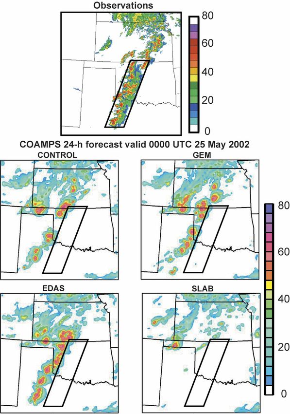
114                                     MONTHLY WEATHER REVIEW                                                       VOLUME 134

1. Introduction

   The effect of land–vegetative processes and the cor-
responding dynamical impact on land–atmosphere in-
teractions is investigated for simulations of the 24–25
May mesoscale convection event that was observed
during the International H2O Project (IHOP_2002)
field experiment (Weckwerth et al. 2004). Land–
vegetative processes, as driven by features such as sur-
face heterogeneity (Pielke 2001) or soil moisture gra-
dients (Zhang and Anthes 1982; Segal et al. 1989;
Chang and Wetzel 1991; Doran and Zhong 1995) have
been shown to be important mechanisms in the devel-
opment of convection. Chang and Wetzel (1991) and
Shaw et al. (1997) show that vegetation gradients can
also be important in the formation of drylines, or nar-
row north–south regions of large horizontal gradients
of atmospheric boundary layer (BL) moisture not as-
sociated with density gradients (McGuire 1962). Strong
gradients in surface fluxes resulting from these inhomo-
geneities can drive mesoscale circulations along the
dryline. Drylines have long been known to be prefer-
ential areas of convection initiation (CI) in the southern
Great Plains (SGP) region (Rhea 1966; Miller 1967;
Schaefer 1986).
   The objective of this study is to investigate the sen-
sitivity of land–vegetative processes in a SGP frontal
and dryline region. This study deals with the impact of
land–atmosphere interactions in strongly forced meso-
scale convection, in contrast to previous work, which
deals with weakly forced synoptic conditions (e.g., Trier
et al. 2004; Clark and Arritt 1995; Segal et al. 1995;
Segal and Arritt 1992; Mahfouf et al. 1987; McCumber
and Pielke 1981). The synoptic forcing dictates the tim-         FIG. 1. COAMPS model domain for (a) 12-km outer nest and
ing and location of the frontal boundaries on the larger       the location of 4-km inner nest, and (b) inner nest terrain (shaded,
                                                               interval of 200 m) and locations of mesonet surface observations
scale. However, the sensitivity of frontal development         (dots) for Oklahoma and west Texas. Amarillo and Shamrock,
and propagation to land–vegetative processes in such a         TX, are indicated by the A and S, respectively.
scenario is not well known. Section 2 describes the ex-
periment design, including the synoptic scenario and
                                                               soscale Prediction System (COAMPS;1 Hodur 1997;
the numerical model simulations. The impact of data
                                                               http://www.nrlmry.navy.mil/coamps-web/web/home/)
assimilation on the initial conditions and forecast char-
                                                               with nonhydrostatic dynamics is used for the numerical
acteristics of the front and dryline is discussed in section
                                                               model simulations. For this study COAMPS is config-
3. The results from the sensitivity simulations are given
                                                               ured with two one-way interactive nests of 12 km (201
in section 4, and the land–atmosphere interactions are
                                                               ⫻ 181 grid points) over the central United States and 4
discussed in section 5.
                                                               km (244 ⫻ 247 grid points) centered over the
                                                               IHOP_2002 observation region (Fig. 1). The emphasis
                                                               is on the higher-resolution 4-km nest, so all subsequent
2. Experiment design
                                                               figures and discussion, with the exception of the synop-
a. COAMPS configuration
  The atmospheric component of the Naval Research                1
                                                                   COAMPS is a registered trademark of the Naval Research
Laboratory’s (NRL) Coupled Ocean/Atmosphere Me-                Laboratory.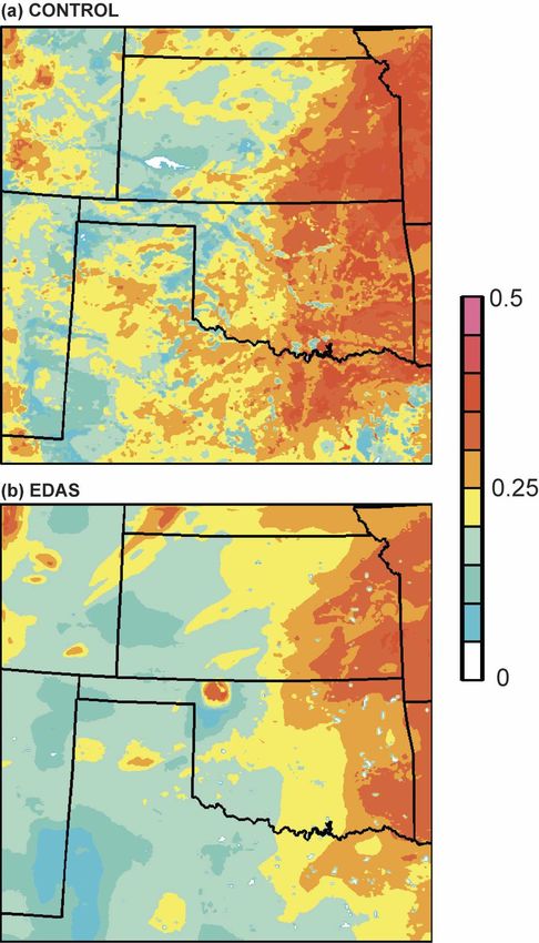
JANUARY 2006                                      HOLT ET AL.                                                        115

tic discussion, will pertain to nest 2. The model has 40         TABLE 1. Description of COAMPS model simulations.
vertical sigma-z levels from 10 to 25 790 m, with in-
                                                                           Land surface       Canopy            Soil
creased vertical resolution in the lower levels. There         Name           model          resistance     assimilation
are 10 levels below 900 m, with the lowest four levels at
                                                             CONTROL       WRF Noah       WRF Noah          HRLDAS
10, 30, 55, and 90 m above ground level (AGL).                                             (Noilhan and
   Four sets of numerical simulations are conducted in                                     Planton 1989)
which three key components—the land surface model,           SLAB          Simple bare    None              None
the canopy resistance/transpiration formulation, and                         soil bulk
                                                             EDAS          WRF Noah       WRF Noah          EDAS
the soil assimilation system—are varied. Table 1 sum-                                      (Noilhan and
marizes the simulations. The control simulation (re-                                       Planton 1989)
ferred to hereafter as CONTROL) includes the                 GEM           WRF Noah       GEM (NAR)         HRLDAS
Weather Research and Forecasting (WRF) Noah land
surface model (LSM), the WRF canopy resistance for-
mulation (Noilhan and Planton 1989; Jacquemin and            has no canopy resistance formulation or soil assimila-
Noilhan 1990), and a soil data assimilation system high-     tion. The initial ground moisture availability is esti-
resolution land data assimilation system (HRLDAS).           mated from the HRLDAS 10-cm soil moisture to pro-
The WRF Noah land surface/hydrology model (Pan               vide similar initial soil conditions as CONTROL.
and Mahrt 1987; Chen et al. 1996; Chen and Dudhia               The simulation EDAS examines the sensitivity to the
2001; Ek et al. 2003) is based on the coupling of the        soil assimilation system. It is the same as CONTROL
diurnally dependent Penman potential evaporation ap-         but replaces the HRLDAS with the coarser 40-km hori-
                                                             zontal resolution (but same vertical resolution) Na-
proach of Mahrt and Ek (1984), the multilayer soil
                                                             tional Centers for Environmental Prediction (NCEP)
model of Mahrt and Pan (1984), and the one-layer
                                                             Eta Data Assimilation (EDAS) operational soil tem-
canopy model of Pan and Mahrt (1987). The canopy
                                                             perature and moisture fields. In contrast to several
resistance formulation has been extended by Chen et
                                                             prior synthetic studies on the sensitivity of drylines to
al. (1996) to include the modestly complex Jarvis-type
                                                             soil moisture by uniformly varying the amount to values
canopy resistance parameterization (Jarvis 1976; Niyogi
                                                             less than 100% (Grasso 2000; Shaw et al. 1997; Ziegler
and Raman 1997).
                                                             et al. 1995), this resolution degradation allows a realis-
   The HRLDAS (Chen et al. 2004; Trier et al. 2004)
                                                             tic assessment of the impact of high-resolution soil
uses observation-based analyses to drive the WRF
                                                             moisture.
Noah LSM in a decoupled mode on the same grids as in
                                                                The simulation GEM examines the sensitivity to the
the coupled atmosphere/LSM model configuration               canopy resistance–transpiration formulation. It is the
(Fig. 1), preventing a mismatch of terrain height, land      same as CONTROL but replaces the WRF Noah for-
use, soil texture, LSM climatology, or LSM physics be-       mulation with a photosynthesis model, the gas ex-
tween HRLDAS and the coupled forecast system. For            change/photosynthesis-based evapotranspiration model
this study the HRLDAS is initialized with data from          (GEM) (Niyogi 2000; Niyogi et al. 2004, manuscript
0000 UTC 1 January 2001, and run uncoupled with four         submitted to J. Appl. Meteor., hereafter NAR). Canopy
soil layers (thickness of each layer from the ground         resistance is a measure of difficulty for soil moisture to
surface to the bottom of 0.1, 0.3, 0.6, and 1.0 m, respec-   be released to the atmosphere via transpiration, which
tively) with a 1-h time step for 18 months, to 24 May        is one of the most efficient means of water loss from the
2002 to reach its equilibrium state. The mesoscale vari-     vegetated land surface.
ability of vegetation and soil characteristics in the re-       The canopy resistance of the WRF Noah scheme is a
gion is illustrated in Fig. 2 showing the COAMPS 4-km        function of minimal stomatal resistance (vegetation-
vegetation categories from the United States Geologi-        type based), leaf area index (calculated after Walko et
cal Survey (USGS) 24-category 30-s dataset and the soil      al. 2000), and effects of solar radiation, water stress,
texture derived from the U.S. Department of Agricul-         vapor pressure deficit, and air temperature as defined
ture 16-category State Soil Geographic Database              in Noilhan and Planton (1989). In GEM the vegetation
(STATSGO).                                                   model is based on the Ball–Woodrow–Berry leaf model
   The simulation SLAB examines the sensitivity to the       (Ball et al. 1987; Niyogi and Raman 1997) and the Col-
land surface model. It uses a bare ground, slab soil         latz et al. (1991, 1992) photosynthesis scheme. The
model with a force–restore surface energy budget with        GEM canopy resistance is calculated as a function of
predictive equations for surface skin temperature and        the net carbon assimilation (photosynthesis) rate, rela-
ground wetness as described in Hodur (1997), and thus        tive humidity, and CO2 concentration at the leaf sur-
116 MONTHLY WEATHER REVIEW VOLUME 134
FIG. 2. COAMPS nest-2 static surface fields of (a) 24-category vegetation and (b) 16-category soil types.
face. Physiological variables at the leaf surface in GEM changes than the WRF Noah scheme, and in turn pro-
are estimated using transpiration/photosynthesis rela- vide quicker thermodynamic changes in the surface
tionships at the leaf scale, and then scaled up using layer (Sellers et al. 1996; Niyogi and Raman 1997;
simple sun-shade and scaling parameterizations as dis- Niyogi et al. 1998; Calvet et al. 1998). This GEM simu-
cussed in Campbell and Norman (1998). A photosyn- lation is one of the first tests of the sensitivity of me-
thesis-based stomatal resistance scheme such as GEM soscale convection to a photosynthesis land surface
is expected to be more responsive to atmospheric scheme.JANUARY 2006 HOLT ET AL. 117
b. Data assimilation deep layer shear over the Oklahoma–Texas panhandle.
The 250-hPa flow (not shown) indicates cyclonic vor-
An initial 2-day spinup is performed for each of the
ticity advection in the same region at 0000 UTC 25
four simulations. A series of 12-h simulations every 12
May.
h from 0000 UTC 22 May to 1200 UTC 23 May 2002 is
performed using intermittent data assimilation in which
routinely available observations are blended with
model first-guess fields using a multivariate optimum 3. Initial conditions and forecasts of the front and
interpolation (MVOI; Barker 1992) scheme after qual- dryline
ity control checks (Baker 1992). For the first simulation
only (0000 UTC 22 May), initial conditions (i.e., model The 2-day data assimilation spinup period prior to
first-guess fields) are obtained by interpolating the 1° the 36-h forecast for each of the four simulations pro-
Navy Operational Global Atmospheric Prediction Sys- vides initial model conditions that more closely re-
tem (NOGAPS) data to the COAMPS domain. Subse- semble observations than simulations initialized from
quent first-guess fields for all other simulations use the just an interpolation of larger-scale data. For example,
previous COAMPS 12-h forecast. After this spinup pe- the positive impact of this spinup on the 24 May initial
riod, a 36-h COAMPS simulation for the period of in- conditions is evident in the CONTROL 0000 UTC sur-
terest from 0000 UTC 24 May 2002 is then performed. face analysis shown in Fig. 4. The surface boundaries
Boundary conditions for all simulations are derived evident in the observations (surface and satellite) in-
from 6-hourly NOGAPS forecasts. clude a weakly defined north–south dryline in west
Figure 1b shows the mesonet surface stations used Texas and the quasi-stationary east–west front extend-
for model validation of low-level temperature, mixing ing through the Oklahoma panhandle northeastward
ratio, winds, and solar radiation (see the IHOP data into southern Kansas (Figs. 4a,b). The front is correctly
management siteat http://www.joss.ucar.edu/ihop/dm/ replicated in the CONTROL analysis except for a slight
for mesonet details). These stations are the 115 Okla- northward displacement in eastern Kansas (Fig. 4c).
homa Mesonet stations (http://www.mesonet.ou.edu/) Likewise, the CONTROL dryline in west Texas is cor-
(of which 100 stations have soil moisture and tempera- rectly positioned considering the 9 g kg⫺1 surface mix-
ture data), and the 28 west Texas Mesonet stations ing ratio contour (Schaefer 1986), with southwesterly
(http://www.mesonet.ttu.edu/). These mesonet data are flow to the west of the dryline and southerly flow to the
not used in the data assimilation and are thus available east. The modeled northeasterly–southwesterly banded
for independent verification of the model forecasts. cloud structure and convective cell near Amarillo,
Texas, also agrees well with observations.
The southeastward movement of the cold front
c. Synoptic scenario across Oklahoma from 1800 UTC 24 May to 0600 UTC
The weather for 24–25 May 2002 over the SGP re- 25 May is depicted by the solid lines in Fig. 4a estimated
gion is dominated by a slow-moving cold frontal system from surface observations. The dryline remains in ap-
and upper-level short-wave trough (Fig. 3). The surface proximately the same location as given in Fig. 4a until
front extends from the Kansas–Oklahoma border to the 0000 UTC 25 May when the cold front moves far
Texas panhandle at 0000 UTC 24 May, with maxima in enough south to merge with the dryline. A comparison
surface moisture convergence along and just south of of model low-level temperatures and moisture to me-
the wind shift as shown in the COAMPS analysis (Fig. sonet observations indicates that all the simulations are
3a). The front slowly moves southeastward, reaching slow in developing and propagating the front. Figure 5
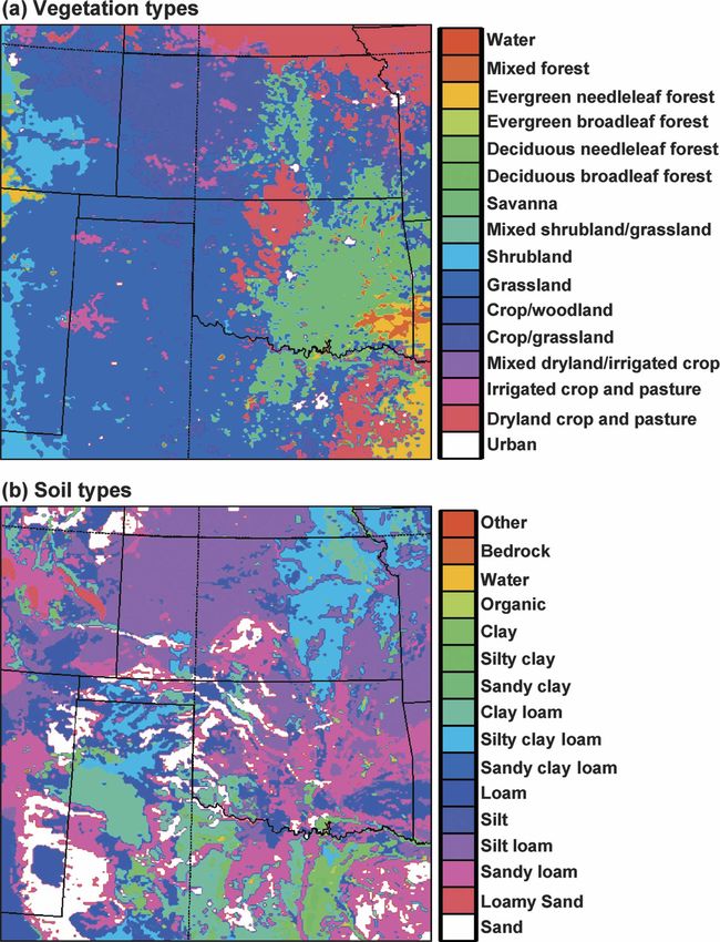
the southeast corner of Oklahoma by 1200 UTC. A low shows the observed and modeled radar reflectivity
pressure center lies over western Texas (1003 hPa at (dBZ ) valid at 0000 UTC 25 May. The box shows the
0000 UTC 24 May and 1007 hPa at 0000 UTC 25 May) estimated orientation of the observed cold-frontal pre-
(Fig. 3c). As is typical of dryline environments in this cipitation band over Oklahoma and north-central
region, there is substantial confluence of moist south- Texas. The simulations with the LSM (CONTROL,
easterly flow from the Gulf of Mexico region with GEM, and EDAS) each show a precipitation band ori-
southwesterly flow from the drier plateaus of southern ented similar to observations, but ⬃100–200 km to the
New Mexico at levels typically below 700 hPa. Between west and lagging by approximately 2–3 h. The SLAB
0000 UTC 24 May and 0000 UTC 25 May, the 500-hPa simulation has not developed convection, indicating
short-wave trough moves eastward and amplifies (Figs. that land surface processes reinforce synoptic processes
3b,d), tightening the height gradients and increasing the to initiate and propagate the frontal precipitation. The118 MONTHLY WEATHER REVIEW VOLUME 134 FIG. 3. COAMPS 12-km analysis valid at 0000 UTC 24 May 2002 of (a) sea level pressure (interval 4 hPa), 10-m wind barbs (full barb ⫽ 5 m s⫺1), regions of surface moisture convergence greater than 7.5 ⫻ 10⫺7 g kg⫺1 s⫺1 (shaded), and estimated surface frontal position; (b) 500-hPa geopotential heights (interval 30 m) and wind barbs, and regions of 700-hPa moisture convergence greater than 7.5 ⫻ 10⫺7 g kg⫺1 s⫺1 (shaded); (c) and (d) same as (a) and (b) except for the COAMPS 24-h forecast valid at 0000 UTC 25 May 2002. synoptics dictate on the larger scale the timing and lo- warm bias from 15 to 24 h. GEM typically shows the cation of the front; however, a proper characterization smallest bias and rmse (⬃1 and ⬃1.5–2.0 K, respec- of land surface processes can be crucial in developing tively) and EDAS and SLAB the largest. A positive the associated convection. bias of surface shortwave radiation for each of the Figure 6 shows the bias and root-mean-square error simulations (maximum of approximately 200 W m⫺2 at (rmse) of 2-m air temperature and mixing ratio for the 2000 UTC) (figure not shown), indicating a general un- four simulations computed using only Oklahoma Me- derprediction of clouds, would account for a large por- sonet surface data located ahead of the observed sur- tion of the warm bias during the daytime. EDAS and face frontal position (see Fig. 4a). This region and time SLAB both show much larger bias and rmse, particu- period (0900 to 2000 LT) is chosen to isolate the model larly from ⬃19 to 24 h (⬃2–3 and ⬃2.5–3.2 K, respec- sensitivity to prefrontal land–atmospheric processes. tively) when convection was prominent along the front. Both model and mesonet observations are averaged The 2-m mixing ratio dry bias prior to approximately 22 over a 1-h time window centered on the hour. For 2-m to 24 h (Fig. 6b) corresponds with the low-level warm temperature statistics (Fig. 6a), all simulations show a bias. For each simulation the bias approaches zero and
JANUARY 2006                                            HOLT ET AL.                                                             119

          FIG. 4. (a) IHOP surface analysis valid at 0000 UTC 24 May 2002 over the COAMPS domain, (b) Geostationary
        Operational Environmental Satellite-8 (GOES-8) visible 1-km-resolution satellite image for 0008 UTC 24 May 2002,
        and (c) CONTROL analysis at 0000 UTC 24 May of 10-m wind barbs (full barb ⫽ 5 m s⫺1), 10-m mixing ratio
        (contour interval ⫽ 1 g kg⫺1), and vertically integrated total cloud fraction (shaded). The subjective locations of
        the cold front and dryline (dashed line) are also given. The dashed box in (c) is the location of the satellite image
        (b) on the COAMPS domain. The estimated observed surface frontal positions at 1800 UTC 24 May (label 18/24
        May), 0000 UTC (label 00/25 May), and 0600 UTC (label 06/25 May) 25 May are given by the solid lines in (a).

the rmse decreases significantly after ⬃26 h when the               indicates that each of the sensitivity experiments have
front and associated convection begins to weaken.                   different distributions from CONTROL. Generally
There is no clear indication of one simulation consis-              SLAB is the driest, showing the largest rmse (indicating
tently performing best; however, for example, the dif-              more large errors), particularly during the afternoon,
ferences in the mean bias and rmse values between the               and GEM is the wettest.
EDAS, SLAB, and GEM and CONTROL are found to                          The statistics for the west Texas dryline region given
be significant at the 95% level at 18, 21, and 24 h using           in Fig. 7 for the time period from 1500 UTC 24 May
a Wilcoxon signed-rank test (Wilks 1995) on the hourly              until it was impacted by the front (2100 UTC) show
mean values from each of the mesonet stations. This                 much larger temperature and moisture bias and rmse
120 MONTHLY WEATHER REVIEW VOLUME 134
FIG. 5. Radar reflectivity (dBZ ) valid at 0002 UTC 25 May for 2-km observations and corresponding 24-h
COAMPS forecasts valid 0000 UTC 25 May. The box shows the estimated orientation of the observed cold-frontal
precipitation band over Oklahoma and north-central Texas.JANUARY 2006 HOLT ET AL. 121
FIG. 6. Time series of (a) 2-m air temperature (°C) and (b) mixing ratio (g kg⫺1) statistics
from 1500 UTC 24 May to 0600 UTC 25 May computed using the Oklahoma surface mesonet
stations shown in Fig. 1b. The statistics are computed in the prefrontal region as shown in Fig. 4a.
for SLAB than the other simulations. SLAB has a large contraction of the mixing ratio field with moisture con-
cold and moist bias (⬃⫺4°–6°C and ⬃3–5 g kg⫺1, re- vergence concentrated along the dryline (not shown).
spectively) and much larger rmse. The markedly differ- Boundary layer depths greater than 2 km AGL are
ent statistical characteristics for SLAB indicate the im- located in the westerly flow behind the dryline and
portance of land–vegetative processes in the LSM, even closely mirror the significantly drier land over the el-
for synoptically driven systems. The impact of land– evated terrain of west Texas and eastern New Mexico.
vegetative processes on model simulations is discussed For SLAB (Fig. 8b) mixing ratios indicate an area of
in section 4. significant humidity gradient in a similar location to
CONTROL, though with a more northeast–southwest
4. Sensitivity to land–vegetative processes orientation, and significantly weaker. The SLAB BL
depth is shallower behind the surface moisture gradi-
a. SLAB simulation ent, with depths over 2 km AGL confined to northeast-
The 21-h forecast of low-level moisture and winds ern New Mexico and not extending into Texas as in
shown in Fig. 8 illustrates some differences between CONTROL. The development of a stronger nocturnal
SLAB and CONTROL. CONTROL shows a classic stable layer through the model data assimilation cycle122 MONTHLY WEATHER REVIEW VOLUME 134
FIG. 7. Time series of statistics similar to Fig. 6, except using the west Texas Mesonet
stations from 1500 to 2100 UTC 24 May in the area of the dryline before passage of the front.
in SLAB limits BL development the following day, as frequently described as a common characteristic of the
similarly noted in modeling studies of Findell and El- dryline (Shaw et al. 1997; Ziegler and Hane 1993;
tahir (2003) and Segal et al. (1995), as well as contrib- Ogura and Chen 1977). CONTROL shows a strong up-
utes to the daytime cold bias (Fig. 7a). The resulting draft core (vertical velocity ⬃0.5–0.8 m s⫺1) concen-
cooler, shallower BL leads to more convective inhibi- trated at the dryline (x ⫽ 260 km on the abscissa),
tion (CIN) west of the dryline for SLAB at 2100 UTC. extending as high as 3.5 km AGL. The BL depth across
Similarly, convective available potential energy the dryline exhibits the classical east–west gradient,
(CAPE) at 2100 UTC is slightly lower for SLAB with depths suppressed to the east (x ⫽ 260 to 500 km),
(⬃1900 J kg⫺1) compared to CONTROL (⬃2600 J with values ⬃1 km AGL with significant vertical gra-
kg⫺1). dients in both and q, and depths to the west (x ⫽ 0 to
Figure 9 shows the vertical structure of virtual poten- 260 km) up to 2.5 to 3 km AGL. The deeper BL to the
tial temperature (), mixing ratio (q), and circulation west results from more rapid heating and from the re-
vectors for the two simulations along the east–west sulting thermally direct circulation. The vertical shear
cross section A–B (shown in Fig. 8). The coinciding associated with strong upper-level (⬃4 km AGL) west-
sharp gradients of and q along the dryline have been erlies to the west (x ⫽ 0 to 260 km) enhances entrain-JANUARY 2006 HOLT ET AL. 123
FIG. 8. The 21-h forecast valid 2100 UTC 24 May of 2-m mixing FIG. 9. Vertical cross section of 21-h forecast valid at 2100 UTC
ratio (contour interval 2 g kg⫺1), 10-m winds (arrows every sev- 24 May along line A–B given in Fig. 8 of mixing ratio (g kg⫺1,
enth grid point, m s⫺1), and boundary layer depth AGL (m, shaded), virtual potential temperature (bold line, interval of 1 K),
shaded) for (a) CONTROL and (b) SLAB. Cross section A–B is and vertical circulation (arrows) for (a) CONTROL and (b)
also indicated along with box S used for averaged fields given in SLAB. The 17–21-h average surface fluxes (W m⫺2) of sensible
Fig. 17. heat (CONTROL: bold dots; SLAB: bold line) and latent heat
(CONTROL: thin dots; SLAB: thin line) along the cross section
are also given.
ment and hence also contributes to deepening and dry-
ing of the BL. turn westerly flow. Within this moisture bulge in
An elevated region of increased moisture, or “mois- CONTROL there exists a distinct vertical rotor circu-
ture bulge” (after Ziegler et al. 1995), is located in the lation with a downdraft core approximately 10 km east
approximately 50-km-wide zone east of the dryline (x ⫽ of the main dryline updraft, similar to that noted by
260 to 310 km) at heights of ⬃1 to 2.5 km AGL for Weiss and Bluestein (2002). The downdraft at x ⬃ 300
CONTROL. This feature has been previously observed km delineates the easterly extent of the ⬃50 km wide
and modeled (Weiss and Bluestein 2002; Atkins et al. bulge.
1998; Ziegler et al. 1995) and associated with the “in- The SLAB vertical circulation (Fig. 9b) is markedly
land sea breeze” circulation. This circulation is charac- different from CONTROL. Though the moisture and
terized by low-level, upslope, moist inflow from the temperature gradients are in approximately the same
southeast (x ⫽ 300–400 km), the strong updraft location as CONTROL (x ⫽ 260 km), and the updraft
core that transports moisture aloft, and upper-level re- strength is comparable, the vertical circulation at the124 MONTHLY WEATHER REVIEW VOLUME 134 gradient and the moisture bulge east of the dryline are absent. The SLAB BL depth is similar to CONTROL east of the gradient zone (x ⫽ 300 to 500 km), but much shallower west of the gradient (x ⫽ 0 to 260 km). The BL is moister to the west as compared to CONTROL because of larger surface latent heat fluxes and less entrainment of dry air. The structure and evolution of the BL responds to changes in fluxes over a period of time, so the 4-h- averaged (17–21 h) latent and sensible heat fluxes along A–B are also shown in Fig. 9. West of the dryline, the largest difference between SLAB and CONTROL is the consistently larger SLAB latent heat fluxes, with values greater than 300 W m⫺2 as compared to ⬃200 W m⫺2 for CONTROL (from x ⫽ 0 to 200 km). Chen et al. (1996) in a comparison of four land evaporation schemes against First International Satellite Land Sur- face Climatology Project (ISLSCP) Field Experiment (FIFE) data noted that the simple slab model overes- timates evaporation during wet periods because of the lack of a canopy resistance to reduce the evaporation to less than the potential rate. This may explain the large moist bias for SLAB shown in Fig. 7b. The BL remains shallow for SLAB to the west of the dryline (Fig. 9b), in spite of larger virtual temperature flux, because of the stronger nocturnal inversion from the previous night and weaker entrainment. These results emphasize the need for physical processes governing moisture in a land surface model via detailed vegetation representa- tion. b. EDAS simulation The primary difference between EDAS and CONTROL is in the soil moisture, illustrated in Fig. 10. FIG. 10. The 21-h forecast of 10-cm volumetric soil moisture Allowing for differences in horizontal resolution, valid at 2100 UTC 24 May for (a) CONTROL and (b) EDAS. EDAS and CONTROL soil moistures are similar in the moister, eastern portion of the domain over eastern gion of largest sensible heat flux and deepest BL for Kansas and Oklahoma, but EDAS is much drier than EDAS occurs along the region extending south- CONTROL over a large region of southwestern Okla- southwest from the southwestern corner of Oklahoma. homa, central Texas, and the Texas panhandle. For ex- This region coincides with the region of enhanced con- ample, in the Texas panhandle, CONTROL values are vective development in EDAS as compared to ⬃0.2 to 0.3, versus 0.1 to 0.2 for EDAS. Subsequently, CONTROL (see Fig. 5). The time–height cross section 10-cm soil temperatures show a corresponding pattern, shown in Fig. 12 of and q at location C in Fig. 11b with EDAS typically 1 to 1.5 K warmer than illustrates the differences in the evolution of the BL CONTROL. It should be noted that these differences between CONTROL and EDAS in this region of large are also generally true for the initial (0000 UTC 24 fluxes. The BL deepens to over 1300 m for EDAS by May) CONTROL versus EDAS soil moistures and 2200 UTC, as compared to only 900 m for CONTROL. temperatures. The 4-h-averaged (17–21 h) EDAS sen- This deepening is a direct response to larger sensible sible heat flux is typically larger than CONTROL over heating for EDAS (sensible heat flux ⬃650 W m⫺2 ver- the drier soil regions (Fig. 11). The larger sensible heat sus 400 W m⫺2 for CONTROL). The effect of warmer, flux regions correlate spatially with larger BL depth drier EDAS soil conditions is greater efficacy in devel- (BL depth 1200-m contour shown in Fig. 11). The re- oping convection due to more radiation partitioning
JANUARY 2006                                           HOLT ET AL.                                                           125

  FIG. 11. Averaged 17–21-h sensible heat flux (W m⫺2) for (a)
CONTROL and (b) EDAS. The contour is the BL depth (1200-m
contour only). Point C is the location for the time–height cross      FIG. 12. Time–height (AGL) cross section at point C shown in
section shown in Fig. 12.                                          Fig. 11 in north-central Texas of virtual potential temperature
                                                                   (shaded) and mixing ratio (solid lines) for (a) CONTROL and
into sensible versus latent heat flux. The preference for          (b) EDAS. The surface heat fluxes during the daytime (15–24 h)
                                                                   illustrate the dominance of sensible to latent for EDAS due to
dry soils to enhance convection in a dryline environ-
                                                                   the drier soil conditions (EDAS 10-cm soil moisture ⬃0.148 vs
ment with such synoptic conditions as occurred for this            0.239 for CONTROL). The evolution of the BL depth indicated
case study agrees with results from Findell and Eltahir            by the dashed line likewise indicates more rapid deepening for
(2003).                                                            EDAS.
  With more extensive development to the southwest,
the region of convection for EDAS shows better agree-
ment with observations (Fig. 5); however, closer exami-            are drier than observations (Fig. 13b), with a bias
nation of thermodynamic variables for the prefrontal               ⬃⫺0.02 to ⫺0.03 (approximately 10% of the magnitude
regions indicates that the warmer and drier EDAS con-              of soil moisture), as compared to ⬃0.01 to 0.017 for
ditions are not as representative of the environment as            CONTROL from 15 to 24 h. Thus, though there is more
CONTROL. For example, statistics computed using                    convective activity in EDAS, this agreement with ob-
Oklahoma Mesonet data for regions ahead of the sur-                servations is fortuitously aided by the anomalously
face front indicate that EDAS soil is much warmer than             warm and dry soil. The HRLDAS assimilation of
observations throughout the period (Fig. 13a) with bi-             CONTROL provides a more realistic depiction of soil
ases 1–2 K and with larger rmse. EDAS soil moistures               conditions than EDAS and hence better overall perfor-
126 MONTHLY WEATHER REVIEW VOLUME 134
FIG. 13. Time series of (a) 10-cm soil temperature (°C) and (b) 10-cm soil moisture (volu-
metric fraction) statistics from 1500 UTC 24 May to 0600 UTC 25 May computed using
prefrontal Oklahoma surface mesonet stations similar to Fig. 6.
mance as indicated by the temperatures and moisture tances show much less spatial variability and less cor-
statistics for the region (see Fig. 6). relation with vegetation variability. This is expected to
contribute to much stronger land–vegetative interac-
c. GEM simulation tion for the GEM resistance scheme. Photosynthesis-
The primary difference between CONTROL and scheme-based resistance formulations, such as GEM,
GEM is illustrated in the 21-h forecast of canopy resis- are generally more responsive to vegetation type, at-
tance to water vapor exchange (Fig. 14). Resistances mospheric conditions, and soil state.
are generally higher in the western part of the domain, The differences in GEM and CONTROL resistances
which is dominated by grassland and shrubs. The cor- affect the model surface heat fluxes via transpiration
responding transpiration rates generally coincide with changes. Figure 15 shows the CONTROL and GEM
resistance variations, with lower resistances resulting in 4-h-averaged (17–21 h) latent heat fluxes. The largest
higher transpiration. The GEM resistances vary with fluxes for both occur in central Oklahoma southward to
vegetation (Fig. 2a), particularly as regards to C3 northeastern Texas where moisture is large and low-
(grasses and trees) versus C4 (certain grasses and level winds are strong from the south (⬃7–8 m s⫺1; see
crops) photosynthesis types. The CONTROL resis- Fig. 8a). Latent heat fluxes for GEM (Fig. 15b) corre-JANUARY 2006 HOLT ET AL. 127
FIG. 15. Averaged 17–21-h latent heat flux (W m⫺2) for (a)
FIG. 14. The 21-h forecast valid 2100 UTC 24 May of canopy
CONTROL and (b) GEM. The contours are for 9 (dashed) and 13
resistance (s m⫺1) for (a) CONTROL and (b) GEM.
g kg⫺1 (solid) 2-m mixing ratio. Differences (model ⫺ obs) of
mixing ratio for five selected mesonet stations are shown (solid
circles) to illustrate the impact of latent heat flux differences.
late spatially with low-resistance areas (Fig. 14b), as
well as regions of larger 2-m mixing ratio (indicated by
the contour lines in Fig. 15b). In contrast, CONTROL variability as represented in the natural variability of
fluxes are less than GEM, less spatially correlated to the vegetation.
the canopy resistances, and show less relationship to
low-level moisture. Differences computed from 2-m 5. Discussion
hourly averaged model and observed mixing ratios
(used in statistics given in Fig. 6b) are also shown for To develop a better understanding of how land–
five Oklahoma Mesonet stations representative of vegetative processes impact the simulation of the dy-
CONTROL and GEM differences (solid circles in Fig. namical response, model results are examined in light
15). The moisture difference is less for each of the sta- of frontogenetic forcing. This is accomplished using the
tions for GEM versus CONTROL (reflected in the re- frontogenesis function as originally proposed by Miller
duced bias in Fig. 6b). Regions in central and western (1948) and used subsequently by others (Sanders 1955;
Oklahoma show the largest improvement (differences Ziegler et al. 1995). The mixing ratio forcing (Fq) is
reduced ⬃1 g kg⫺1), where fluxes are generally larger considered here because of its importance in defining
for GEM than CONTROL, with much more spatial the dryline:128 MONTHLY WEATHER REVIEW VOLUME 134
FIG. 16. Vertical cross section of 2000–2100 UTC 24 May averaged forcing terms of mixing
ratio frontogenesis (⫻10⫺7 g kg m⫺1 s⫺1) of (top) horizontal deformation, (middle) tilting, and
(bottom) total for (a) CONTROL, (b) SLAB, (c) GEM, and (d) EDAS along line A–B. Dark
regions are frontogenetic areas and light regions are frontolytic. Contours are maximum
horizontal boundary layer wind (m s⫺1) along the cross section in (a), maximum vertical
velocity (m s⫺1) in (b), and mixing ratio (interval of 2 g kg⫺1) in (c).
Fq ⫽ ⫺共hq兲⫺1再冋 冉 冊 冉 冊 冉 冊 冉 冊 册
⭸q
⭸x
2 ⭸u
⭸x
⫹
⭸q
⭸y
2 ⭸
⭸y
Figure 16 shows the two forcing terms for CONTROL,
SLAB, GEM, and EDAS for the cross section along
A–B in Fig. 8. Forcing for LSM simulations (CONTROL,
⫹ 冋冉 冊冉 冊冉 冊册 冋冉 冊冉 冊
⭸q
⭸x
⭸q
⭸y
⭸ ⭸u
⫹
⭸x ⭸y
⫹
⭸q
⭸x
⭸q
⭸p
GEM, and EDAS) shows that horizontal deformation
(Fhdef) strongly increases the low-level moisture gradi-
ent at the dryline (x ⫽ 260 km) up to a height ranging
⫻ 冉 冊 冉 冊冉 冊冉 冊册冎
⭸
⭸x
⫹
⭸q
⭸y
⭸q
⭸p
⭸
⭸y
, 共1兲
from 2 to 2.5 km AGL (Fig. 16, top panels). The maxi-
mum horizontal BL wind along the cross section
(shown schematically in top panels) is ⫾3 to 4 m s⫺1
where the time tendency has been neglected following concentrated below 1 km AGL within 100 km either
Ziegler et al. (1995) because the soil moisture gradients side of the dryline for the LSM simulations. The con-
are on a larger scale than the dryline. The first two tribution from tilting is also largest for the LSM simu-
terms on the right-hand side of (1) represent the hori- lations, concentrated at elevations ⬃1–3 km AGL
zontal deformation (Fhdef), and the third is the tilting (Fig. 16, middle). The EDAS simulation has the largest
term (Ftilt). tilting-based forcing in connection with stronger differ-JANUARY 2006 HOLT ET AL. 129
FIG. 16. (Continued)
ential vertical velocity (strongest updrafts ⬃1.1 m s⫺1 and only weakly frontogenetic at the BL top (⬃1 km
and downdrafts ⬃⫺0.4 m s⫺1). The elevated frontoge- AGL), several orders of magnitude less than CONTROL.
netic/frontolytic tilting–forcing couplet from x ⫽ 260 to Correspondingly, there is little BL convergence with
310 km for the LSM simulations coincides with the el- regions of maximum BL wind displaced more than 100
evated moisture bulge discussed previously, indicating km from the dryline and weaker (⬃2 to 3 m s⫺1) than
the importance of the updraft/downdraft couplet in the LSM simulations. Here Ftilt is at least one order of
turning the vapor gradient into the vertical and main- magnitude smaller than CONTROL, concentrated at
taining the sharp gradients. The resulting total fronto- the BL top, and strongest at the dryline and to the west
genesis for CONTROL, GEM, and EDAS (Fig. 16, (x ⫽ 75 to 200 km), but with much less vertical extent
bottom) shows strong boundary layer frontogenetic than in CONTROL due to the lack of an elevated mois-
forcing due to convergence along the dryline, resulting ture bulge. Likewise the differential vertical velocity is
in the significant scale contraction evident in the mois- reduced compared to LSM simulations. The resulting
ture gradient. The tilting term dominates total forcing SLAB total forcing resembles the nonclassical dryline
at and above the BL top, with the only other significant characteristics described in Segal and Arritt (1992).
forcing outside the 50-km dryline zone evident due to Neither convergent forcing nor tilting is present to
tilting at the BL top. maintain a sharp moisture gradient.
The SLAB simulation is significantly different in its Figure 17 illustrates the land–atmosphere feedback
frontogenetic characteristics. At the moisture gradient of EDAS, GEM, and SLAB relative to CONTROL
at x ⫽ 260 km, Fhdef is virtually nonexistent in the BL averaged over a 1-h period from 2000 to 2100 UTC for130 MONTHLY WEATHER REVIEW VOLUME 134
FIG. 17. Percent change of quantities for simulations GEM, EDAS, and SLAB relative to
CONTROL values averaged from 2000 to 2100 UTC 24 May 2002 over the 60 km ⫻ 60 km
Shamrock, TX, subset region (given by box S in Fig. 8a). Positive percent changes indicate an
increase relative to the CONTROL values. This time is considered prefrontal, with no pre-
cipitation for any simulation from 2000 to 2100 UTC.
a 60 km ⫻ 60 km region near Shamrock, Texas (box S temperature/moisture changes. In GEM the larger
in Fig. 8a). The purpose of this comparison is to em- canopy resistance reduces transpiration, reducing the
phasize the relative importance of land–vegetative pro- release of moisture to the atmosphere and thus increas-
cesses under similar synoptic forcing (i.e., clear sky and ing soil moisture. For EDAS the soil moisture/soil tem-
prefrontal). For the comparison time and for all simu- perature change can be considered as the direct effect
lations, this region is south of the front and there is no and the associated changes in the transpiration/canopy
precipitation. The surface is a mixture of grassland and resistance as feedback. EDAS soil moisture is 7% less
bare ground. While some of the differences may still be than CONTROL, which contributes to warmer soil (via
a function of synoptic situation, careful choice of the emissivity and albedo feedbacks in the model param-
area should ensure that most of the differences are re- eterization). The combined effect of the soil moisture/
lated to differences in the treatment of the surface vari- soil temperature and canopy resistance changes con-
ables. tributes to the overall reduction in transpiration. For
As shown in Fig. 17, the canopy resistance for GEM this region, the small vegetation cover (42%) reduces
is almost 500% larger than CONTROL and almost the importance of transpiration relative to evaporation
50% larger for EDAS (SLAB does not include vegeta- from the soil. Thus, for GEM the nearly 60% reduction
tion response). Larger vegetation resistances correlate in transpiration translates to only a 36% reduction in
directly with less transpiration and indirectly with soil latent heat flux. However, the 6% reduction in EDASJANUARY 2006 HOLT ET AL. 131
transpiration corresponds to a 7% reduction in latent ally timing and amount of precipitation at a particular
heat flux because of the additional effect of lowered soil location.
moisture. For SLAB the latent heat flux changes very This analysis supports the premise that including ad-
little (1%) compared to CONTROL. For sensible heat vanced photosynthetic processes in a mesoscale model
flux the most significant change is the almost 25% in- will produce stronger coupling between the surface and
crease for GEM. the overlying surface and boundary layers. On the
The changes in the surface layer response propagate other hand, EDAS results are responsive to changes in
into the BL. For GEM and EDAS the 2-m air tempera- the soil moisture but these changes do not necessarily
tures are much warmer and the mixing ratios much produce as strong a boundary layer response. The
drier than CONTROL (0.3 K and 0.4 K %, an increase EDAS surface feedback is somewhat limited because
of ⬃1 K; ⫺12% and ⫺11%, a decrease of ⬃1.5 g kg⫺1). even though the surface has altered soil moisture/soil
The SLAB air temperature is cooler by 0.43 K % (more temperature, the response to the surface layer and the
than 1 K) in response to a shallower BL depth (by 36%) atmosphere has to be through the vegetation/transpira-
that entrains less warm air from above. The BL is tion scheme, which in this case is relatively less inter-
deeper by 5%–10% in GEM and EDAS, with warming active with fewer variables as compared to the photo-
and drying near the surface correlated with a deeper synthesis-based GEM.
BL. Mesoscale BL vertical velocities show the largest
reduction for SLAB (43%), supporting a generally
6. Conclusions
shallower, moister, and less energetic BL. CAPE is also
the smallest for SLAB (⫺28%), though each of the Numerical model simulations are conducted to un-
simulations has sufficient CAPE to support convection derstand the effect of land–atmosphere interactions on
(values range form 1900 to 2600 J kg⫺1), owing to the a mesoscale convective event over the southern Great
synoptic forcing. It is the increase in CIN for SLAB Plains during IHOP_2002 characterized by strong
(113%) that precludes the development of convection. dryline synoptic forcing in conjunction with a quasi-
The LSM simulations show similar values of CIN, with stationary cold-frontal system. Variations to the speci-
GEM the smallest. Boundary layer cloud cover is less fication of land surface model (LSM), canopy resis-
than 4% coverage for all simulations for this relatively tance formulation, and type and resolution of soil as-
cloud free, prefrontal region. similation system are examined. Each of the LSM
In summary, changes in canopy resistance affect tran- simulations develops convection 2–3 h after observed,
spiration, which in turn modulates the water loss from as synoptic-scale forcing determines the location and
the surface (and hence soil moisture). The changes in timing of the frontal boundaries on the large scale.
soil moisture affect the emissivity and albedo and can Simulations with the LSM develop convection in ap-
impact soil temperature. Indeed, the canopy resistance proximately the correct location and much earlier than
and transpiration depend on the soil temperature and the simulation using a simpler slab surface model. The
soil moisture. As discussed in Niyogi et al. (2002), the slab model also has larger low-level temperature and
soil–vegetation coupling is relative to the soil moisture moisture biases and root-mean-square errors computed
availability (i.e., larger soil moisture availability results from mesonet data over Oklahoma and west Texas.
in greater interaction between vegetation and soil, and Thus, the physical parameterizations in the slab model
hence systematic transpiration and soil moisture are insufficient to properly account for land–vegetative
changes). Changes in the surface characteristics alter processes such as those occurring along the dryline and
the surface fluxes for sensible and latent heat. This in frontal boundaries in this case.
turn modifies the air temperature and moisture content Coarser-resolution soil data (EDAS) that is generally
of the surface layer/lower boundary layer. The response drier and warmer than the high-resolution land data
propagates upward through the boundary layer via tur- assimilation system (HRLDAS) used in the control
bulent transport and affects boundary layer growth. In simulation provides an environment more conducive
turn, the growth of the boundary layer leads to engulf- for convection (larger CAPE and less CIN). Thus, the
ment of warm and dry air above the boundary layer and development of convection in association with the
at the same time dilutes the effect of surface heating dryline is typically more extensive for EDAS than
(since the same amount of heating spreads through a CONTROL. However, statistics computed from meso-
larger depth; see, e.g., LeMone et al. 2000). These pro- net data show soil moisture and temperature biases (as
cesses change the CAPE and CIN, and in conjunction well as air temperature and moisture during the pre-
with other mesoscale feedbacks contribute to the fron- frontal period) are larger using the coarser-resolution
togenetic forcing, boundary layer clouds, and eventu- EDAS data compared to HRLDAS. Thus, land–132 MONTHLY WEATHER REVIEW VOLUME 134
vegetative processes in EDAS are forced by anoma- hydrology model with the Penn State–NCAR MM5 modeling
lously warmer and drier conditions than observed. system. Part I: Model implementation and sensitivity. Mon.
Wea. Rev., 129, 569–585.
An advanced representation of photosynthesis-based
——, and Coauthors, 1996: Modeling of land-surface evaporation
evapotranspiration shows improvements in predictive by four schemes and comparison with FIFE observations. J.
skill for 2-m air temperature and moisture. This is be- Geophys. Res., 101, 7251–7268.
cause model soil moisture changes by themselves (such ——, K. W. Manning, D. N. Yates, M. A. LeMone, S. B. Trier, R.
as those tested by using a different soil assimilation Cuenca, and D. Niyogi, 2004: Development of a High Reso-
system like EDAS) do not directly affect the coupled lution Land Data Assimilation System (HRLDAS). Pre-
prints, 16th Conf. on Numerical Weather Prediction, Seattle,
land–atmosphere response. Rather, the atmosphere re- WA, Amer. Meteor. Soc., CD-ROM, 22.3.
sponds to changes in soil moisture via latent heat flux, Clark, C. A., and R. W. Arritt, 1995: Numerical simulations of the
boundary layer growth, heating/cooling, CIN, and effect of soil moisture and vegetation cover on the develop-
CAPE. This manifestation of the changes in the sur- ment of deep convection. J. Appl. Meteor., 34, 2029–2045.
face/subsurface details on the soil moisture/tempera- Collatz, G. J., J. Ball, C. Grivet, and J. Berry, 1991: Physiological
and environmental regulation of stomatal conductance, pho-
ture is more effectively achieved by enhancing the veg-
tosynthesis, and transpiration: A model that includes a lami-
etation/transpiration scheme (as in GEM). This is be- nar boundary layer. Agric. For. Meteor., 54, 107–136.
cause transpiration is the most efficient means of water ——, M. Ribas-Carbo, and J. Berry, 1992: Coupled photosynthe-
vapor exchange from the surface to the atmosphere. sis–stomatal conductance model for leaves of C4 plants. Aust.
J. Plant Physiol., 19, 519–538.
Acknowledgments. The research was supported by Doran, J. C., and S. Zhong, 1995: Variations in mixed-layer depths
the Program Element 0602435N of the Naval Research arising from inhomogeneous surface conditions. J. Climate, 8,
1965–1973.
Laboratory Base Program Project Number BE-435-
Ek, M. B., K. E. Mitchell, Y. Lin, E. Rogers, P. Grunmann, V.
003; NSF-ATM 0233780 (Dr. S. Nelson), the NASA– Koren, G. Gayno, J. D. Tarpley, 2003: Implementation of
THP (NNG04GI84G, Dr. J. Entin), and the NASA- Noah land surface model advances in the National Centers
IDS (NNG04GL61G, Drs. J. Entgin and G. Gutman). for Environmental Prediction operational mesoscale Eta
The IHOP_2002 data collection and processing were Model. J. Geophys. Res., 108, 8851, doi:10.1029/2002JD003296.
Findell, K. L., and E. A. B. Eltahir, 2003: Atmospheric controls on
supported by the NCAR Water Cycle Initiatives and by
soil moisture–boundary layer interactions. Part II: Feedbacks
NSF/NCAR USWRP funds. The first author would like within the continental United States. J. Hydrometeor., 4, 570–
to thank James Doyle for many fruitful discussions and 583.
suggestions for improving the manuscript. Also thanks Grasso, L. D., 2000: A numerical simulation of dryline sensitivity
to Joseph Alfieri and Steve Williams for help in pro- to soil moisture. Mon. Wea. Rev., 128, 2816–2834.
cessing IHOP_2002 data and Dr. Stan Trier for an in- Hodur, R. M., 1997: The Naval Research Laboratory’s Coupled
Ocean/Atmosphere Mesoscale Prediction System (COAMPS).
sightful review.
Mon. Wea. Rev., 125, 1414–1430.
Jacquemin, B., and J. Noilhan, 1990: Sensitivity study and valida-
REFERENCES tion of a land surface parameterization using the HAPEX-
MOBILHY data set. Bound.-Layer Meteor., 52, 93–134.
Atkins, N. T., R. M. Wakimoto, and C. L. Ziegler, 1998: Ob-
Jarvis, P. G., 1976: The interpretation of the variations in leaf
servations of the finescale structure of a dryline during
water potential and stomatal conductance found in canopies
VORTEX95. Mon. Wea. Rev., 126, 525–550.
in the field. Philos. Trans. Roy. Soc. London, B273, 593–610.
Baker, N. L., 1992: Quality control for the navy operational at-
mospheric database. Wea. Forecasting, 7, 250–261. LeMone, M. A., and Coauthors, 2000: Land–atmosphere interac-
Ball, J., I. Woodrow, and J. Berry, 1987: A model predicting sto- tion research, early results, and opportunities in the Walnut
matal resistance and its contribution to the control of photo- River Watershed in southeast Kansas: CASES and ABLE.
synthesis under different environmental conditions. Progress Bull. Amer. Meteor. Soc., 81, 757–779.
in Photosynthesis Research, J. Biggins, Ed., Vol. IV, Martinus Mahfouf, J.-F., E. Richard, and P. Mascart, 1987: The influence of
Nijhoff, 221–224. soil and vegetation on the development of mesoscale circu-
Barker, E. H., 1992: Design of the navy’s multivariate optimum lations. J. Climate Appl. Meteor., 26, 1483–1495.
interpolation analysis system. Wea. Forecasting, 7, 220–231. Mahrt, L., and M. Ek, 1984: The influence of atmospheric stability
Calvet, J.-C., J. Noilhan, J. Roujean, P. Bessemoulin, M. Cabel- on potential evaporation. J. Climate Appl. Meteor., 23, 222–
guenne, A. Olioso, and J. Wigneron, 1998: An interactive 234.
vegetation SVAT model tested against data from six con- ——, and H. L. Pan, 1984: A two-layer model of soil hydrology.
trasting sites. Agric. For. Meteor., 92, 73–95. Bound.-Layer Meteor., 29, 1–20.
Campbell, G. S., and J. M. Norman, 1998: An Introduction to En- McCumber, M. C., and R. A. Pielke, 1981: Simulation of the ef-
vironmental Biophysics. 2d ed. Springer, 312 pp. fects of surface fluxes of heat and moisture in a mesoscale
Chang, J.-T., and P. J. Wetzel, 1991: Effects of spatial variations of numerical model. Part I: Soil layer. J. Geophys. Res., 86,
soil moisture and vegetation on the evolution of a prestorm 9929–9938.
environment: A case study. Mon. Wea. Rev., 119, 1368–1390. McGuire, E. L., 1962: The vertical structure of three drylines as
Chen, F., and J. Dudhia, 2001: Coupling an advanced land surface/ revealed by aircraft traverses. National Severe Storms Proj-JANUARY 2006 HOLT ET AL. 133
ect Rep. 7, 11 pp. [Available from NCAR, P.O. Box 3000, lations caused by surface sensible heat flux gradients. Bull.
Boulder, CO 80307.] Amer. Meteor. Soc., 73, 1593–1604.
Miller, J. E., 1948: On the concept of frontogenesis. J. Meteor., 5, ——, W. E. Schreiber, G. Kallos, J. R. Garratt, A. Rodi, J.
169–171. Weaver, and R. A. Pielke, 1989: The impact of crop areas in
Miller, R. C., 1967: Notes on analysis and severe-storm forecasting northeast Colorado on midsummer mesoscale thermal circu-
procedures of the Military Weather Warning Center Tech. lations. Mon. Wea. Rev., 117, 809–825.
Rep. 200, U.S. Air Force Air Weather Service, Scott Air ——, R. Arritt, C. Clark, R. Rabin, and J. Brown, 1995: Scaling
Force Base, IL, 170 pp. evaluation of the effect of surface characteristics on potential
Niyogi, D. S., 2000: Biosphere–atmosphere interactions coupled for deep convection over uniform terrain. Mon. Wea. Rev.,
with carbon dioxide and soil moisture changes. Ph.D. disser- 123, 383–400.
tation, North Carolina State University, 509 pp. Sellers, P., S. O. Los, C. J. Tucker, C. O. Justice, D. A. Dazlich,
——, and S. Raman, 1997: Comparison of four different stomatal G. J. Collatz, and D. A. Randall, 1996: A revised land surface
resistance schemes using FIFE observations. J. Appl. Meteor., parameterization (SiB2) for atmospheric GCMs. Part II: The
36, 903–917. generation of global fields of terrestrial biophysical param-
——, K. Alapaty, and S. Raman, 1998: Comparison of four dif- eters from satellite data. J. Climate, 9, 706–737.
ferent stomatal resistance schemes using FIFE observations. Shaw, B. L., R. A. Pielke, and C. L. Ziegler, 1997: A three-
Part II: Analysis of terrestrial biospheric–atmospheric inter- dimensional numerical simulation of a Great Plains dryline.
actions. J. Appl. Meteor., 37, 1301–1320. Mon. Wea. Rev., 125, 1489–1506.
——, Y.-K. Xue, and S. Raman, 2002: Hydrological land surface Trier, S. B., F. Chen, and K. W. Manning, 2004: A study of con-
response in a tropical regime and a midlatitudinal regime. J. vection initiation in a mesoscale model using high-resolution
Hydrometeor., 3, 39–56. land surface initial conditions. Mon. Wea. Rev., 132, 2954–
Noilhan, J., and S. Planton, 1989: A simple parameterization of 2976.
land surface processes for meteorological models. Mon. Wea. Walko, R. L., and Coauthors, 2000: Coupled atmosphere–
Rev., 117, 536–549. biophysics–hydrology models for environmental modeling. J.
Ogura, Y., and Y. Chen, 1977: A life history of an intense meso- Appl. Meteor., 39, 931–944.
scale convective storm in Oklahoma. J. Atmos. Sci., 34, 1458– Weckwerth, T. M., and Coauthors, 2004: An overview of the In-
1476. ternational H2O Project (IHOP_2002) and some preliminary
Pan, H.-L., and L. Mahrt, 1987: Interaction between soil hydrol- highlights. Bull. Amer. Meteor. Soc., 85, 253–277.
ogy and boundary-layer development. Bound.-Layer Meteor., Weiss, C. C., and H. B. Bluestein, 2002: Airborne pseudo–dual
38, 185–202. Doppler analysis of a dryline–outflow boundary intersection.
Pielke, R. A., 2001: Influence of the spatial distribution of veg- Mon. Wea. Rev., 130, 1207–1226.
etation and soils on the prediction of cumulus convective Wilks, D. S., 1995: Statistical Methods in the Atmospheric Sciences.
rainfall. Rev. Geophys., 39, 151–177. Academic Press, 467 pp.
Rhea, J. O., 1966: A study of thunderstorm formation along Zhang, D., and R. A. Anthes, 1982: A high-resolution model of
drylines. J. Appl. Meteor., 5, 58–63. the planetary boundary layer—Sensitivity tests and compari-
Sanders, F., 1955: An investigation of the structure and dynamics son with SESAME-79 data. J. Appl. Meteor., 21, 1594–1609.
of an intense surface frontal zone. J. Meteor., 12, 542–552. Ziegler, C. L., and C. E. Hane, 1993: An observational study of
Schaefer, J. T., 1986: The dryline. Mesoscale Meteorology and the dryline. Mon. Wea. Rev., 121, 1134–1151.
Forecasting, P. S. Ray, Ed., Amer. Meteor. Soc., 549–570. ——, W. J. Martin, R. A. Pielke, and R. L. Walko, 1995: A mod-
Segal, M., and R. W. Arritt, 1992: Nonclassical mesoscale circu- eling study of the dryline. J. Atmos. Sci., 52, 263–285.You can also read