Z-GCNETs: Time Zigzags at Graph Convolutional Networks for Time Series Forecasting
←
→
Page content transcription
If your browser does not render page correctly, please read the page content below
Z-GCNETs: Time Zigzags at Graph Convolutional Networks
                             for Time Series Forecasting

                             Yuzhou Chen 1 2 Ignacio Segovia-Dominguez 3 4 Yulia R. Gel 3 2

                          Abstract                                   1. Introduction
                                                                     Many real world phenomena are intrinsically dynamic by
       There recently has been a surge of interest in de-            nature, and ideally neural networks, encoding the knowl-
       veloping a new class of deep learning (DL) archi-             edge about the world should also be based on more explicit
       tectures that integrate an explicit time dimension            time-conditioned representation and learning mechanisms.
       as a fundamental building block of learning and               However, most currently available deep learning (DL) ar-
       representation mechanisms. In turn, many recent               chitectures are inherently static and do not systematically
       results show that topological descriptors of the              integrate time-dimension into the learning process. As a
       observed data, encoding information on the shape              result, such model architectures often cannot reliably, ac-
       of the dataset in a topological space at different            curately and on time learn many salient time-conditioned
       scales, that is, persistent homology of the data,             characteristics of complex interdependent systems, resulting
       may contain important complementary informa-                  in outdated decisions and requiring frequent model updates.
       tion, improving both performance and robustness
       of DL. As convergence of these two emerging                   In turn, in the last few years we observe an increasing in-
       ideas, we propose to enhance DL architectures                 terest to integrate deep neural network architectures with
       with the most salient time-conditioned topologi-              persistent homology representations of the learned objects,
       cal information of the data and introduce the con-            typically in a form of some topological layer in DL (Hofer
       cept of zigzag persistence into time-aware graph              et al., 2019; Carrière et al., 2020; Carlsson & Gabrielsson,
       convolutional networks (GCNs). Zigzag persis-                 2020). Such persistent homology representations allow us to
       tence provides a systematic and mathematically                extract and learn descriptors of the object shape. (By shape
       rigorous framework to track the most important                here we broadly understand data characteristics that are in-
       topological features of the observed data that tend           variant under continuous transformations such as bending,
       to manifest themselves over time. To integrate the            stretching, and compressing.) Such interest in combining
       extracted time-conditioned topological descrip-               persistent homology representations with DL is explained
       tors into DL, we develop a new topological sum-               by the complementary multi-scale information topological
       mary, zigzag persistence image, and derive its the-           descriptors deliver about the underlying objects, and higher
       oretical stability guarantees. We validate the new            robustness of these salient object characterisations to pertur-
       GCNs with a time-aware zigzag topological layer               bations.
       (Z-GCNETs), in application to traffic forecasting             Here we take the first step toward merging the two direc-
       and Ethereum blockchain price prediction. Our                 tions. To enhance DL with the most salient time-conditioned
       results indicate that Z-GCNET outperforms 13                  topological information, we introduce the concept of zigzag
       state-of-the-art methods on 4 time series datasets.           persistence into time-aware DL. Building on the fundamen-
                                                                     tal results on quiver representations, zigzag persistence stud-
                                                                     ies properties of topological spaces which are connected
   1
     Department of Statistical Science, Southern Methodist Univer-   via inclusions going in both directions (Carlsson & Silva,
sity, TX, USA 2 Energy Storage & Distributed Resources Division,     2010; Tausz & Carlsson, 2011; Carlsson, 2019). Such gen-
Lawrence Berkeley National Laboratory, CA, USA 3 Department
of Mathematical Sciences, University of Texas at Dallas, TX,         eralization of ordinary persistent homology allows us to
USA 4 NASA Jet Propulsion Laboratory, CA, USA. Correspon-            track topological properties of time-conditioned objects by
dence to: Yuzhou Chen , Ignacio Segovia             extracting salient time-aware topological features through
Dominguez , Yulia R.          time-ordered inclusions. We propose to summarize the
Gel .                                              extracted time-aware persistence in a form of zigzag persis-
Proceedings of the 38 th International Conference on Machine         tence images and then to integrate the resulting information
Learning, PMLR 139, 2021. Copyright 2021 by the author(s).           as a learnable time-aware zigzag layer into GCN.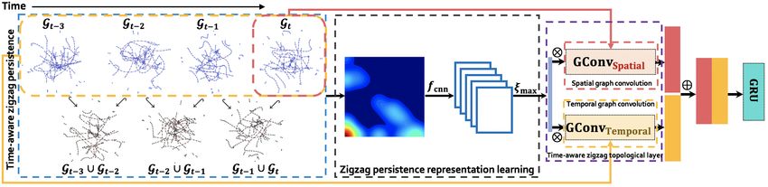
Z-GCNETs: Time Zigzags at Graph Convolutional Networks for Time Series Forecasting

The key novelty of our paper can be summarized as follows:       RNN are limited by the underlying structure of the input
                                                                 data, for instance, these methods are not designed to han-
   • This is the first approach bridging time-conditioned DL     dle objects from non-Euclidean spaces, such as graphs and
     with time-aware persistent homology representations         manifolds.
     of the data.
                                                                 Graph convolutional networks To overcome the limita-
   • We propose a new vectorized summary for time-aware          tions of traditional convolution on graph structured data,
     persistence, namely, zigzag persistence image and dis-      graph convolution-based methods (Defferrard et al., 2016;
     cuss its theoretical stability guarantees.                  Kipf & Welling, 2017; Veličković et al., 2018) are proposed
                                                                 to explore both global and local structures. GCNs usually
   • We introduce the concepts of time-aware zigzag persis-      consists of graph convolution layers which extract the edge
     tence into learning time-conditioned graph structures       characteristics between neighbor nodes and aggregate fea-
     and develop a zigzag topological layer (Z-GCNET) for        ture information from neighborhood via graph filters. In
     time-aware graph convolutional networks (GCNs).             addition to convolution, there has been a surge of interest
   • Our experiments on application Z-GCNET to traffic           in applying GCNs to time series forecasting tasks (Yu et al.,
     forecasting and Ethereum blockchain price prediction        2018; Yao et al., 2018; Yan et al., 2018; Guo et al., 2019;
     show that Z-GCNET surpasses 13 state-of-the-art meth-       Weber et al., 2019; Pareja et al., 2020; Segovia Dominguez
     ods on 4 benchmark datasets, both in terms of accuracy      et al., 2021). Although these methods have achieved state-
     and robustness.                                             of-the-art performance in traffic flow forecasting, human
                                                                 action recognition, and anti-money laundering regulation,
                                                                 the design of spatial temporal graph convolution network
2. Related Work                                                  framework is mostly based on modeling spatial-temporal
Zigzag Persistence is yet an emerging tool in applied            correlation in terms of feature-level and pre-defined graph
topological data analysis, but many recent studies have al-      structure.
ready shown its high utility in such diverse applications
as brain sciences (Chowdhury et al., 2018), imagery clas-        3. Time-Aware Topological Signatures of
sification (Adams et al., 2020), cyber-security of mobile           Graphs
sensor networks (Adams & Carlsson, 2015; Gamble et al.,
2015), and characterization of flocking and swarming be-         Spatio-temporal Data as Graph Structures The spatial-
havior in biological sciences (Corcoran & Jones, 2017; Kim       temporal networks can be represented as a sequence
et al., 2020). An alternative to zigzag but a closely related    of discrete snapshots, {G1 , G2 , . . . , GT }, where Gt =
approach to assess properties of time-varying data with per-     {Vt , Et , Wt } is the graph structure at time step t, t =
sistent homology, namely, crocker stacks, has been recently      1, . . . , T . In Gt , Vt is a node set with cardinality |Vt | of Nt
suggested by Xian et al. (2020), though the crocker stacks       and Et ⊆ Vt × Vt is an edge set. A nonnegative symmetric
                                                                                                             t
representations are not learnable in DL models. While            Nt × Nt -matrix Wt with entries {ωij          }1≤i,j≤Nt represents
                                                                                                             t
zigzag has been studied in conjunction with dynamic sys-         the adjacency matrix of Gt , that is, ωij      > 0 for any etij ∈ Et
                                                                           t
tems (Tymochko et al., 2020) and time-evolving point             and ωij = 0, otherwise. Let F, F ∈ Z>0 be the number
clouds (Corcoran & Jones, 2017), till now, the utility of        of different node features associated each node v ∈ Vt .
zigzag persistence remains untapped not only in conjunc-         Then, a Nt × F feature matrix X t serves as an input to the
tion with GCNs but with any other DL tools.                      framework of time series process modeling. Throughout
                                                                 the paper we suppress subscript t, for the sake of notations,
Time series forecasting From a deep learning perspective,        unless dependency over time is emphasized in the particular
Recurrent Neural Networks (RNNs) are natural methods to          context.
model time-dependent datasets (Yu et al., 2019). In partic-
ular, the stable architecture of Long Short Term Memories        Background on Persistent Homology Persistent homol-
(LSTMs), and its variant called Gate Recurrent Unit (GRU),       ogy is a mathematical machinery to extract the intrin-
solves the gradient instability of predecessors and adds extra   sic shape properties of graph G that are invariant under
flexibility due to their memory storage and forget gates. The    continuous transformations such as bending, stretching,
ability of LSTM and GRU to selectively learn historical          and twisting. The key idea is, based on some appropri-
patterns led to their wide spread adoption as one of the main    ate scale parameter, to associate G with a graph filtration
DL tools for time-dependant objects (Schmidhuber, 2017;          G 1 ⊆ . . . ⊆ G n = G and then to equip each G i with an
Shin & Kim, 2020; Segovia-Dominguez et al., 2021). In            abstract simplicial complex C (G i ), 1 ≤ i ≤ n, yielding
general, GRU models tend to have fewer parameters than           a filtration of complexes C (G 1 ) ⊆ . . . ⊆ C (G n ). Now,
LSTMs but exhibit similar forecasting performance (Greff         we can systematically and efficiently track evolution of
et al., 2017; Gao et al., 2020). However, applications of        various patterns such as connected components, cycles,
Z-GCNETs: Time Zigzags at Graph Convolutional Networks for Time Series Forecasting
and voids throughout this hierarchical sequence of com- sions over time
plexes. Each topological feature, or p-hole (e.g., number
of connected components and voids), 0 ≤ p ≤ D, is rep- G1 G2 G3 . . .
,!
,!
resented by a unique pair (ib , jd ), where birth ib and death ,
,!
,!
jd are the scale parameters at which the feature first ap- G1 ∪ G 2 G2 ∪ G 3
pears and disappears, respectively, and D is the highest
dimension of the simplicial complexes. The lifespan of the where Gk ∪ Gk+1 is defined as a graph with a node set
feature is defined as jd − ib . The extracted topological in- Vk ∪ Vk+1 and an edge set Ek ∪ Ek+1 . Second, we fix a
formation can be then summarized as a persistence diagram scale parameter ν∗ and build a zigzag diagram of simpli-
Dgm = {(ib , jd ) ∈ R2 |ib < jd }. Multiplicity of a point cial complexes for the given ν∗ over the constructed set of
(ib , jd ) ∈ D is the number of p-dimensional topological fea- network inclusions
tures (p-holes) that are born and die at ib and jb , respectively. C (G1 , ν∗ ) C (G2 , ν∗ )
Points at the diagonal Dgm are taken with infinite multiplic-
,!
,!
,!
ity. The idea is then to evaluate topological features that
persist (i.e., have longer lifespan) over the complex filtra- C (G1 ∪ G2 , ν∗ ) ...
tion and, hence, are likelier to contain important structural
Using the zigzag filtration for the given ν∗ , we can track
information on the graph.
birth and death of each topological feature over {Gt }T1 as
Finally, filtration of the weighted graph G can be con- time points tb and td , 1 ≤ tb ≤ td ≤ T , respectively.
structed in multiple ways. For instance, (i) we can select Similarly to a non-dynamic case, we can extend the no-
a scale parameter as a shortest weighted path between any tion of persistence diagram for the analysis of topological
two nodes; then as an abstract simplicial complex C on characteristics of time-varying data delivered by the zigzag
G, consider a Vietoris–Rips (VR) complex V R ν∗ (G) = persistence.
0 0
{G ⊆ G|diam(G ) ≤ ν∗ }. That is, Vietoris-Rips complex Definition 3.1 (Zigzag Persistence Diagram (ZPD)). Let
0
V R ν∗ (G) is generated by subgraphs G of bounded diame- tb and td be time points, when a topological feature first
0 0
ter ν∗ (i.e. any subgraph G of k-nodes with diam(G ) ≤ ν∗ appears (i.e., is born) and disappears (i.e., dies) in the time
generates a (k − 1)-simplex in V R ν∗ (G)). Hence, for a period [1, T ] over the zigzag diagram of simplicial com-
set of scale thresholds ν1 ≤ . . . ≤ νn , we obtain a VR plexes for a fixed scale parameter ν∗ , respectively. If the
filtration V R 1 ⊆ . . . ⊆ V R n . Alternatively, (ii) we can topological feature first appears in C (Gk , ν∗ ), tb = k; if it
consider a sublevel filtration induced by a continuous func- first appears in C (Gk ∪Gk+1 , ν∗ ), tb = k+1/2. Similarly, if
tion f defined on the nodes set V of G. Let f : V ! R and a topological feature last appears in C (Gk , ν∗ ), td = k; and
ν1 < ν2 < . . . < νn be a sequence of sorted filtered values, if it last appears in C (Gk ∪Gk+1 , ν∗ ), td = k+1/2. A multi-
then C i = {σ ∈ C : maxv∈σ f (v) ≤ νi }. Note that a set of points in R2 , DgmZZν∗ = {(tb , td ) ∈ R2 |tb < tb },
VR filtration (i) is a subcase of sublevel filtration (ii) with for a fixed ν∗ is called a zigzag persistence diagram (ZPD).
f being the diameter function (Adams et al., 2017; Bauer,
2019). Inspired by the notion of a persistent image as a summary
of ordinary persistence (Adams et al., 2017), to input topo-
Time-Aware Zigzag Persistence Since our primary aim
logical information summarized by ZPD into a GCN, we
is to assess interconnected evolution of multiple time-
propose a representation of ZPD as zigzag persistence image
conditioned objects, the developed methodology for track-
(ZPI). ZPI is a finite-dimensional vector representation of a
ing topological and geometric properties of these objects
ZPD and can be computed through the following steps:
shall ideally account for their intrinsically dynamic nature.
We address this goal by introducing the concept of zigzag
• Step 1: Map a zigzag persistence diagram DgmZZν∗ to an
persistence into GCN. Zigzag persistence is a generaliza-
integrable function ρDgmZZν∗ : R2 ! R2 , called a zigzag
tion of persistent homology proposed by (Carlsson & Silva,
persistence surface. The zigzag persistence surface is
2010) and provides a systematic and mathematically rig-
given by sums of weighted Gaussian functions that are
orous framework to track the most important topological
centered at each point in DgmZZν∗ , i.e.
features of the data persisting over time.
||z−µ||2
Let {Gt }T1 be a sequence of networks observed over time.
X
ρDgmZZν∗ = g (µ) e − 2ϑ2 .
The key idea of zigzag persistence is to evaluate pairwise µ∈DgmZZ0ν∗
compatible topological features in this time-ordered se-
quence of networks. First, we define a set of network inclu- Here DgmZZ0ν∗ is the transformed multi-set in DgmZZν∗ ,
i.e., DgmZZ0ν∗ (x, y) = (x, y − x); g(µ) is a weighting
function with mean µ = (µx , µy ) ∈ R2 and variance ϑ2 ,
which depends on the distance from the diagonal.Z-GCNETs: Time Zigzags at Graph Convolutional Networks for Time Series Forecasting
• Step 2: Perform a discretization of a subdomain of zigzag 4. Z-GCNETs
persistence surface ρDgmZZν∗ in a grid.
Given the graph G and graph signals X τ =
{X t−τ , . . . , X t−1 } ∈ Rτ ×N ×F of τ past time pe-
• Step 3: The ZPI, i.e., a matrix of pixel values, can be
riods (i.e. window size τ ; where X i ∈ RN ×F and
obtained by subsequent integration over each grid box.
i ∈ {t − τ, . . . , t − 1}), we employ a model targeted
on multi-step time series forecasting. That is, given the
The value of each pixel z ∈ R2 within a ZPI is then defined windows size τ of past graph signals and the ahead horizon
as: size h, our goal is to learn a mapping function which maps
ZZ X ||z−µ||2 the historical data {X t−τ , . . . , X t−1 } into the future data
ZPIν∗ (z) = g (µ) e − 2ϑ2 dzx dzy . {X t , . . . , X t+h }.
z µ∈DgmZZ0ν∗
Laplacianlink In spatial-temporal domain, the topology
of graph may have different structure at different points
Proposition 3.1. Let g : R2 ! R be a non-negative contin- in time. In this paper, we use the self-adaptive adjacency
uous and piece-wise differentiable function. Let DgmZZν∗ matrix (Wu et al., 2019) as the normalized Laplacian by
be a zigzag persistence diagram for some fixed scale parame- trainable node embedding dictionaries φ ∈ RN ×c , i.e.,
ter ν∗ , and let ZPIν∗ be its corresponding zigzag persistence L = sof tmax(ReLU (φφ> )), where the dimension of
image. Then, ZPIν∗ is stable with respect to the Wasserstein- embedding c ≥ 1. Although introducing node embedding
1 distance between zigzag persistence diagrams. dictionaries allows capture hidden spatial dependence in-
formation, it cannot sufficiently capture the global graph
Derivations of the proposition can be found in Appendix D information and the similarity between nodes. To overcome
of the supplementary material. the limits and explore neighborhoods of nodes at differ-
Tracking evolution of topological patterns in these se- ent depths, we define a new polynomial representation for
quences of time-evolving graphs allows us to glean insights Laplacian based on positive powers of the Laplacian matrix.
into which properties of the observed time-conditioned ob- Laplacianlink L̃ is then formulated as:
jects, e.g., traffic data or Ethereum transaction graphs, tend h i
to persist over time and, hence, are likelier to play a more L̃ = I, L, L2 , . . . , LK ∈ RN ×N ×(K+1) , (1)
important role in predictive tasks.
where K ≥ 1, I ∈ RN ×N represents the identity matrix,
and Lk ∈ RN ×N , with 0 ≤ k ≤ K, denotes the power
series of normalized Laplacian.
By linking (i.e., stacking) the power series of normalized
Laplacian, we build a diffusion formalism to accumulate
neighbors’ information of different power levels. Hence,
each node will successfully exploit and propagate spatial-
temporal correlations after spatial and temporal graph con-
volutional operations.
Spatial graph convolution To model the spatial network Gt
at timestamp t with its node feature matrix X t , we define the
spatial graph convolution as multiplying the input of each
layer with the Laplacianlink L̃, which is then fed into the
trainable projection matrix Θ = φV (where V stands for
the trainable weight). In spatial-temporal graph modeling,
we prefer to use weight sharing in matrix factorization rather
than directly assigning a trainable weight matrix in order not
only to avoid the risk of over-fitting but also to reduce the
computational complexity. We compute the transformation
in spatial domain, in each layer, as follows:
Figure 1. Illustrations of 0- and 1-dimensional ZPD and 0- and (`) (`−1) >
1-dimensional ZPI for PeMSD4 dataset using the sliding window H i,S = (L̃H i,S ) φV , (2)
size τ = 12, i.e., dynamic network with 12 graphs. Upper part
shows the 0-dimensional ZPD and ZPI whilst the lower part is the where φ ∈ RN ×c is the node embedding and V ∈
1-dimensional ZPD and ZPI. Rc×(K+1)×Cin ×(Cout /2) is the trainable weight (Cin andZ-GCNETs: Time Zigzags at Graph Convolutional Networks for Time Series Forecasting
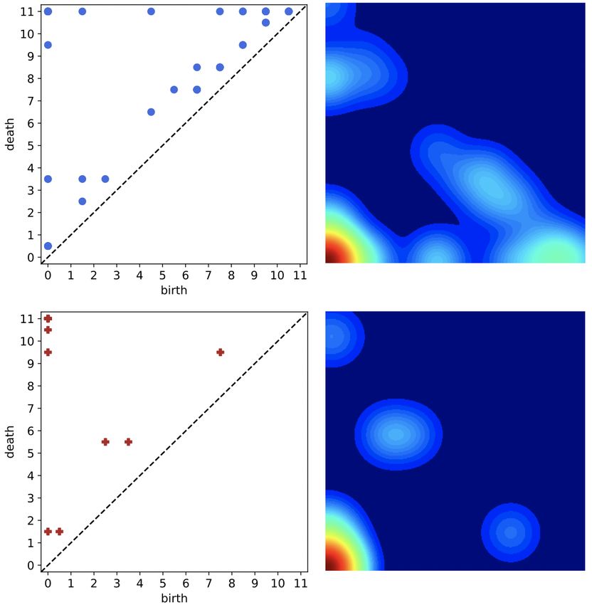
Figure 2. The architecture of Z-GCNETs. Given a sliding window, e.g. (Gt−3 , . . . , Gt ), we extract zigzag persistence image (ZPI) based
on zigzag filtration. For the ZPI ∈ R2 with the shape of p × p, Z-GCNETs first learn the topological features of ZPI through CNN-based
framework, and then apply global max-pooling to obtain the maximum values among pooled activation maps. The output of zigzag
persistence representation learning is decoded into spatial graph convolution and temporal graph convolution, where the inputs of spatial
graph convolution and temporal graph convolution are current timestamps, e.g., Gt in red dashed box, and the sliding window (i.e.,
(Gt−3 , . . . , Gt ) in yellow dashed box) respectively. After graph convolution operations, features from time-aware zigzag topological layer
are combined and moved to GRU to perform forecasting. Symbol ⊗ represents dot product whilst ⊕ denotes combination.
Cout are the number of channels in input and output, re- sliding window X τ . (Here for brevity we suppress de-
(`−1)
spectively). Finally, H i,S ∈ RN ×(Cin /2) is the matrix pendence of ZPI on a scale parameter ν∗ .) We design the
of activations of spatial graph convolution to the `-th layer time-aware zigzag topological layer to (i) extract and learn
(0) the spatial-temporal topological features contained in ZPI,
and H i,S = X i . As a result, all information regarding
the `-layered input at time i are reflected in the latest state (ii) aggregate transformed information from (spatial or tem-
variable. poral) graph convolution and spatial-temporal topological
information from zigzag persistence module, and (iii) mix
Temporal graph convolution In addition to spatial domain, spatial-temporal and spatial-temporal topological informa-
the nature of spatial-temporal networks includes temporal tion. The information’s extraction, aggregation, and combi-
relationships among multiple spatial networks. To extract nation processes are expressed as:
temporal dependency patterns, we choose longer window
size (i.e., by using the entire sliding window as input) and
apply temporal graph convolution to graph signals in sliding
window X τ . The mechanism has several excellent prop- Z (`) = ξmax fcnn
(`)
(ZPIτ ) ,
erties: (i) there is no need to select a particular size of the (`) (`)
Si = H i,S Z (`) ,
nested sliding window, (ii) temporal dependency patterns (4)
(`) (`)
can be well captured and evaluated by (longer) window Ti = H i,T Z (`) ,
sizes, whereas shorter window sizes (i.e., nested sliding (`) (`) (`)
H i,out = COMBINE(`) (S i , T i ),
window) are likelier to be biased and noisy, and (iii) the slid-
ing window X τ enhances efficiency of estimating temporal
dependencies. The temporal graph convolution is given by:
(`)
where fcnn represents the convolutional neural network
(`) (`−1)
H i,T = (L̃H i,T )> φU (`−1) Q, (3) (CNN) in the `-th layer, ξmax (·) denotes global max-pooling
operation, Z (`) ∈ R(Cout /2) is the learned zigzag persis-
where U (`) ∈ Rc×Cin ×(Cout /2) is trainable weight and (`)
tence representation from CNN, S i ∈ RN ×(Cout /2) is
U (0) ∈ Rc×F ×(Cout /2) , Q ∈ Rτ ×1 is the trainable pro- 2
the aggregated spatial -temporal representation, T i ∈
(`)
jection vector in temporal graph convolutional layer, and 2
RN ×(Cout /2) is the aggregated spatial-temporal represen-
(`−1)
H i,T ∈ Rτ ×N ×(Cin /2) is the hidden matrix fed to the tation, and the output of time-aware zigzag topological layer
(0) (`) (`) (`)
`-th layer and H i,T = X τ ∈ Rτ ×N ×F . H i,out ∈ RN ×Cout combines hidden states S i and T i
at time i.
Time-aware zigzag topological layer To learn the topolog-
ical features across a range of spatial and temporal scales, GRU with time-aware zigzag topological layer GRU is a
we extend the CNN model to be used along with ZPI. In variant of the LSTM network. Compared with LSTM, GRU
this paper, we present a framework to aggregate the topo- has a simpler structure, fewer training parameters, and more
logical persistent features into the feature representation easily overcome vanishing and exploding gradient problems.
learned from GCN. Let ZPIτ denote the ZPI based on the The feed forward propagation of GRU with time-awareZ-GCNETs: Time Zigzags at Graph Convolutional Networks for Time Series Forecasting
et al., 2001) collects real time traffic data in California. Both
Table 1. Summary of datasets used in time series forecasting tasks.
PeMSD4 and PeMSD8 datasets are aggregated to 5 minutes,
[‡] means the average number of edges in transportation networks
under threshold ν∗ . therefore there are overall 16,992 and 17,856 data points in
PeMSD4 and PeMSD8, respectively. In the traffic network,
Dataset # Nodes Avg # edges Time range
the node is represented by the loop detector which can detect
Bytom 100 9.98 27/07/2017 - 07/05/2018 real time measurement of traffic conditions and the edge
Decentraland 100 16.94 14/10/2017 - 07/05/2018 is a freeway segment between two nearest nodes. Hence,
PeMSD4 307 316.10‡ 01/01/2018 - 28/02/2018 the node set Vt ≡ V and the node feature matrix of traffic
PeMSD8 170 193.53‡ 01/07/2016 - 31/08/2016 network Xt ∈ RN ×3 denotes that each node has 3 features
(i.e., flow rate, speed, and occupancy) at time t. To capture
both spatial and temporal dependencies, we reconstruct the
zigzag topological layer is recursively conducted as: traffic graph structure Gt = {V, Et , Wtν∗ } at time t. Here,
we define the right censoring weight Wtν∗
z i = ϕ (W z [O i−1 , H i,out ] + bz ) ,
r i = ϕ (W r [O i−1 , H i,out ] + br ) , wt,uv (u, v) ∈ E and wt,uv ≤ ν∗
(5) ν∗
ωt,uv = 0 (u, v) ∈ E and wt,uv > ν∗ , (6)
Õ i = tanh (W o [r i O i−1 , H i,out ] + bo ),
0 (u, v) ∈
/E
Õ i = z t O i−1 + (1 − z t ) Õ i ,
2
where ϕ(·) is a non-linear function, i.e., the ReLU function; where wt,uv = e−||xt,u −xt,v || /γ is based on the Radial Ba-
is the elementwise product; z i and r i are update gate sis Function (RBF). To investigate how the traffic graph
and reset gate, respectively; bz , br , bo , W z , W r , and W o structure evolves over time, at each time point t we keep
ν∗
are trainable parameters; [O i−1 , H i,out ] and O i are the only edges with weights ωt,uv which are no greater than
input and output of GRU model, respectively. In this way, some positive threshold ν∗ . Hence, the resulting graph is dy-
Z-GCNETs contains structural, temporal, and topological namic, that is, its edge set changes over the considered time
information. period. In our experiments, we assign parameter γ = 1.0
to RBF and set the thresholds in PeMSD4 and PeMSD8 to
Figure 2 depicts the framework of our proposed Z-GCNETs ν∗ = 0.5 and ν∗ = 0.3, respectively. (ii) The Ethereum
model. As illustrated in Figure 2, Z-GCNETs contains the blockchain was developed in 2014 to implement Smart Con-
four major steps. First, we use CNN base model (fcnn ) tracts, which are used to create and sell digital assets on the
to learn the topological features of an ZPI and then em- network1 . In particular, token assets are specially valuable
ploy global max-pooling (ξmax ) to the corresponding feature because each token naturally represents a network layer
maps to obtain image-level feature representation (see the with the same nodes, i.e., addresses of users, appearing in
black dashed box). Second, purple dashed box, in the spa- the networks, i.e., layers, of multiple tokens (Akcora et al.,
tial and temporal dimensions, i.e., (i) we use spatial graph 2021; Li et al., 2020; di Angelo & Salzer, 2020). For our
convolution to capture spatial correlations between nodes experiments, we extract two token networks with more than
and get H S (Equation 2); (ii) we use temporal graph con- $100M in market value2 , Bytom and Decentraland tokens,
volution to capture temporal correlations between features from the publicly available Ethereum blockchain. We focus
in different time slices and get H T (Equation 3). Third, we our analysis on the dynamic network generated by the daily
can get hidden states S (red dashed block) and T (yellow transactions on each token network, and historical daily
dashed block) by applying the H S and H T to ZPI repre- closed prices2 . Since each token has different creation date3 ,
sentation, respectively; then combine S and T and get output Bytom dynamic network contains 285 nets whilst Decen-
of time-aware zigzag topological layer H out (Equation 4). traland dynamic network has 206 nets. Ethereum’s token
Fourth, we pass H out to the GRU for modeling the temporal networks have an average of 442788/1192722 nodes/edges.
dependency. To maintain a reasonable computation time, we obtain a
subgraph via the maximum weight subgraph approximation
5. Experiments method of (Vassilevska et al., 2006), which allows us to re-
duce the dynamic network size considering only most active
5.1. Datasets nodes and its corresponding nodes. Let Gt = {Vt , Et , W̃t }
We consider two types of networks (i) traffic network and denotes the reduced Ethereum blockchain network on day t
(ii) Ethereum token network. Statistical overview of all and Xt ∈ RNt ×1 be the node feature matrix, we assume a
datasets is given in Table 1. We now describe the detailed solely node feature: the node degree. Each node in Vt is a
construction of traffic and Ethereum transaction networks as 1
Ethereum.org
follows (i) The freeway Performance Measurement System 2
EtherScan.io
3
(PeMS) data sources (i.e., PeMSD4 and PeMSD8) (Chen End date: May 7, 2018Z-GCNETs: Time Zigzags at Graph Convolutional Networks for Time Series Forecasting
Table 2. Forecasting performance comparison of different approaches on PeMSD4 and PeMSD8 datasets. The baselines with † marks the
results from rerunning the published source codes. Z-GCNETs uses the weight rank clique filtration.
PeMSD4 PeMSD8
Model
MAE RMSE MAPE MAE RMSE MAPE
HA 38.03 59.24 27.88% 34.86 52.04 24.07%
VAR (Hamilton, 2020) 24.54 38.61 17.24% 19.19 29.81 13.10%
FC-LSTM† (Sutskever et al., 2014) 26.77 40.65 18.23% 23.09 35.17 14.99%
GRU-ED (Cho et al., 2014) 23.68 39.27 16.44% 22.00 36.23 13.33%
DSANet (Huang et al., 2019) 22.79 35.77 16.03% 17.14 26.96 11.32%
DCRNN† (Li et al., 2018) 21.20 37.23 14.15% 16.83 26.35 10.90%
STGCN† (Yu et al., 2018) 21.16 35.69 13.83% 17.52 27.07 11.23%
GraphWaveNet† (Wu et al., 2019) 28.15 39.88 18.52% 20.30 30.82 13.84%
ASTGCN† (Guo et al., 2019) 22.81 34.33 16.60% 17.98 28.00 11.66%
MSTGCN† (Guo et al., 2019) 23.96 37.21 14.33% 19.00 29.15 12.38%
STSGCN† (Song et al., 2020) 21.23 33.69 13.90% 17.13 26.86 10.96%
AGCRN† (Bai et al., 2020) 19.83 32.30 12.97% 15.95 25.22 10.09%
LSGCN (Huang et al., 2020) 21.53 33.86 13.18% 17.73 26.76 11.20%
Z-GCNETs (ours) 19.50 31.61 12.78% 15.76 25.11 10.01%
buyer/seller and edges in Et represent transactions in the net- PeMSD8 datasets. Besides, the inputs of PeMSD4 and
work. To construct the similarity matrix W̃t , the normalized PeMSD8 are normalized by min-max normalization ap-
number of transactions between node pairs (u, v) serves as proach. We split Bytom and Decentraland with 80% for
the edge weight value wt,uv ∈ W̃t . In our experiments, we
consider a set of 100 most actively trading nodes over the
whole time period. That is, on each particular day t, both
the node and edge sets vary. If a particular node vi does not Table 3. Computational costs for generation of zigzag persistence
trade on day t, then vi is entered as isolated node. As such, images (ZPI) and a single training epoch of Z-GCNETs.
N = 100. Average Time Taken (sec)
Dataset Window Size
ZPI Z-GCNETs (epoch)
5.2. Experiment Settings
Decentraland 7 0.03 2.09
For multi-step time series forecasting, we evaluate the per- Bytom 7 0.03 2.06
formances of Z-GCNETs on 4 time series datasets versus 13 PeMSD4 12 0.86 30.12
state-of-the-art baselines (SOAs). Among them, Historical PeMSD8 12 0.65 36.76
Average (HA) and Vector Auto-Regression (VAR) (Hamil-
ton, 2020) are the statistical time series models. FC-
LSTM (Sutskever et al., 2014) and GRU-ED (Cho et al.,
2014) are RNN-based neural networks. DSANet (Huang training sets and 20% for test sets. For token networks,
et al., 2019) is the self-attention networks. DCRNN (Li et al., Z-GCNETs contains 2 layers, where each layer has 16
2018), STGCN (Yu et al., 2018), GraphWaveNet (Wu et al., hidden units. We use one week historical data to predict
2019), ASTGCN (Guo et al., 2019), MSTGCN (Guo et al., the next week’s data, i.e., window size τ = 7 and hori-
2019), STSGCN (Song et al., 2020) are the spatial-temporal zon h = 7 over Bytom and Decentralnad datasets. All
GCNs. AGCRN (Bai et al., 2020) and LSGCN (Huang reported results are based on the weight rank clique filtra-
et al., 2020) are the GRU-based GCNs. We conduct our tion (Stolz et al., 2017). More detailed description of the
experiments on NVIDIA GeForce RTX 3090 GPU card experimental settings can be found in Appendix A, while
with 24GB memory. The PeMSD4 and PeMSD8 are split the analysis of sensitivity with respect to the choice of fil-
in chronological order with 60% for training sets, 20% for tration is in Appendix B. The code is available at https:
validation sets, and 20% for test sets. For PeMSD4 and //github.com/Z-GCNETs/Z-GCNETs.git.
PeMSD8, Z-GCNETs contains 2 layers, with each layer
Table 3 reports the average running time of ZPI generation
has 64 hidden units. We consider the window size τ = 12
and training time per epoch of our Z-GCNETs model on all
and horizon h = 12 for Z-GCNETs on both PeMSD4 and
datasets.Z-GCNETs: Time Zigzags at Graph Convolutional Networks for Time Series Forecasting
5.3. Comparison with the Baseline Methods Comparison results on PeMSD8, w/o zigzag learning and
w/o show the necessity for encoding topological information
Table 2 shows the comparison of our proposed Z-GCNETs
and modeling spatial structural information in multi-step
and SOAs for traffic flow forecasting tasks. We assess model
forecasting over spatial-temporal time series datasets. Addi-
performance with Mean Absolute Error (MAE), Root Mean
tional results for the ablation study on Ethereum tokens are
Square Error (RMSE), and Mean Absolute Percentage Error
presented in Appendix C.
(MAPE) on PeMSD4 and PeMSD8. From Table 2, we find
that our proposed model Z-GCNETs consistently outper-
forms SOAs on PeMSD4 and PeMSD8. The improvement Table 5. Ablation study of the network architecture. [*] means
gain of Z-GCNETs over the next most accurate methods the GCNSpatial is only applied to the most recent time point in the
ranges from 0.44% to 2.06% in RMSE for PeMSD4 and sliding window.
PeMSD8. Table 4 summarizes the forecasting performance Architecture MAE RMSE MAPE
on Bytom and Decentraland in terms of RMSE.
Z-GCNETs 19.50 31.61 12.78%
We find that Z-GCNETs, based on the power filtration with W/o Zigzag learning 19.65 31.94 13.01%
PeMSD4
transaction volume as edge weight, outperforms AGCRN by W/o GCNSpatial ∗ 19.86 31.96 13.19%
margins of 3.67% and 4.60%. (See the results in Appendix B W/o GCNTemporal 20.76 33.18 13.60%
for other filtrations. For all filtration types, Z-GCNETs
yields better forecasting performance than all SOAs.). In Z-GCNETs 15.76 25.11 10.01%
contrast with SOAs, Z-GCNETs fully leverages the topologi- W/o Zigzag learning 17.16 27.06 10.77%
PeMSD8
cal information by incorporating zigzag topological features W/o GCNSpatial ∗ 16.92 26.86 10.33%
via CNN on topological space. Given the dynamic nature W/o GCNTemporal 16.66 26.44 10.39%
of the considered data, our experiments show that estab-
lishing a connection between the time-indexed zigzag pairs
can deliver substantial gains for learning and forecasting 5.5. How does time-aware zigzag persistence help?
time-evolving objects.
To track the importance of p-dimensional topological fea-
tures in Z-GCNETs (i.e., 0-dimensional and 1-dimensional
Table 4. Forecasting results (MAPE) on Ethereum token networks. holes), we evaluate the performance of Z-GCNETs on two
Z-GCNETs uses power filtration with transaction volume as edge different aspects: (i) the sensitivity of Z-GCNETs to differ-
weight. ent dimensional topological features and (ii) the effects of
Model Bytom Decentraland threshold ν∗ in constructed input networks along with zigzag
persistence. Table 6 summarizes the results using different
FC-LSTM (Sutskever et al., 2014) 40.72% 33.46%
dimensional topological features and different thresholds on
DCRNN (Li et al., 2018) 35.36% 27.69%
PeMSD4 and PeMSD8. Under the same scale parameter
STGCN (Yu et al., 2018) 37.33% 28.22%
ν∗ , we find that 1-dimensional topological features con-
GraphWaveNet (Wu et al., 2019) 39.18% 37.67%
sistently outperform 0-dimensional terms on both datasets.
ASTGCN (Guo et al., 2019) 34.49% 27.43%
Furthermore, the forecasting results on PeMSD4 are not
AGCRN (Bai et al., 2020) 34.46% 26.75%
significantly affected by varying ν∗ . However, on PeMSD8,
LSGCN (Huang et al., 2020) 34.91% 28.37%
1-dimensional topological features constructed under ν∗ of
Z-GCNETs 30.79% 22.15% 0.3 yield better results than 1-dimensional summaries con-
structed under ν∗ = 0.5.
5.4. Ablation Study 5.6. Robustness Study
To better understand the importance of the different com- To assess robustness of Z-GCNETs under noisy conditions,
ponents in Z-GCNETs, we conduct ablation studies on we consider adding Gaussian noise into 30% of training sets.
PeMSD4 and PeMSD8 and the results are presented in Ta- The added noise follows zero-mean i.i.d Gaussian density
ble 5. The results show that Z-GCNETs have better perfor- with fixed variance ς 2 , i.e., N (0, ς 2 ), where ς ∈ {2, 4}. In
mance over Z-GCNETs without zigzag persistence represen- Table 7, we report comparisons with two competitive base-
tation learning (zigzag learning), spatial graph convolution lines (AGCRN and LSGCN) on Decentraland and PeMSD4
(GCNSpatial ), or temporal graph convolution (GCNTemporal ). using two different noise levels. Table 7 shows performance
Specifically, we observe that when removing GCNTemporal , of Z-GCNETs and two SOAs under described noisy con-
the multi-step forecasting is affected significantly, i.e., Z- ditions. We find that performance of all methods slowly
GCNETs outperforms Z-GCNETs without temporal graph decays as variance of noise increases. Nevertheless, we
convolution with relative gain 6.46% on RMSE for PeMSD4. notice that Z-GCNETs is still consistently more robust thanZ-GCNETs: Time Zigzags at Graph Convolutional Networks for Time Series Forecasting
or recommendations expressed in this material are those of
Table 6. Results of zigzag persistence on the dynamic network
the author(s) and do not necessarily reflect the views of the
with different dimensional features and threshold values (ν∗ ).
Office of Naval Research. The authors are grateful to Baris
PeMSD4 Coskunuzer for insightful discussions.
Zigzag module
MAE RMSE MAPE
0-th ZPIν∗ =0.3 19.73 32.04 12.93% References
1-st ZPIν∗ =0.3 19.47 31.66 12.75% Adams, H. and Carlsson, G. Evasion paths in mobile sen-
Z-GCNETs +
0-th ZPIν∗ =0.5 19.78 32.20 12.98% sor networks. The International Journal of Robotics
1-st ZPIν∗ =0.5 19.50 31.61 12.78% Research, 34(1):90–104, 2015.
PeMSD8 Adams, H., Emerson, T., Kirby, M., Neville, R., Peterson,
Zigzag module
MAE RMSE MAPE C., Shipman, P., Chepushtanova, S., Hanson, E., Motta,
F., and Ziegelmeier, L. Persistence images: A stable
0-th ZPIν∗ =0.3 17.14 27.24 10.66%
vector representation of persistent homology. Journal of
1-st ZPIν∗ =0.3 15.76 25.11 10.01%
Z-GCNETs + Machine Learning Research, 18, 2017.
0-th ZPIν∗ =0.5 17.22 27.41 10.77%
1-st ZPIν∗ =0.5 16.77 26.62 10.39% Adams, H., Bush, J., Carr, B., Kassab, L., and Mirth, J. A
torus model for optical flow. Pattern Recognition Letters,
129:304–310, 2020.
SOAs on both Decentraland and PeMSD4.
Akcora, C. G., Kantarcioglu, M., and Gel, Y. R. Blockchain
networks: Data structures of bitcoin, monero, zcash,
Table 7. Robustness study on Decentraland and PeMSD4 (RMSE). ethereum, ripple and iota. arXiv:2103.08712, 2021.
Noise AGCRN LSGCN Z-GCNETs (ours)
Bai, L., Yao, L., Li, C., Wang, X., and Wang, C. Adaptive
N (0, 2) 27.69 36.10 24.12 graph convolutional recurrent network for traffic forecast-
Decentraland
N (0, 4) 28.12 36.79 25.03 ing. Advances in Neural Information Processing Systems,
33, 2020.
N (0, 2) 32.24 34.16 31.95
PeMSD4
N (0, 4) 32.67 34.75 32.18 Bauer, U. Ripser: efficient computation of vietoris-rips
persistence barcodes. arXiv:1908.02518, 2019.
Carlsson, G. Persistent homology and applied homotopy
6. Conclusion theory. Handbook of Homotopy Theory, 2019.
Inspired by the recent call for developing time-aware deep Carlsson, G. and Gabrielsson, R. B. Topological approaches
learning mechanisms of the US Defense Advanced Re- to deep learning. In Topological Data Analysis, pp. 119–
search Projects Agency (DARPA), we have proposed a new 146. Springer, 2020.
time-aware zigzag topological layer (Z-GCNETs) for time- Carlsson, G. and Silva, V. Zigzag persistence. Found.
conditioned GCNs. Our idea is based on the concepts of Comput. Math., 10(4):367–405, August 2010. ISSN 1615-
zigzag persistence whose utility remains unexplored not 3375.
only in conjunction with time-aware GCN but DL in general.
The new Z-GCNETs layer allows us to track the salient time- Carrière, M., Chazal, F., Ike, Y., Lacombe, T., Royer, M.,
aware topological characterizations of the data persisting and Umeda, Y. Perslay: A neural network layer for per-
over time. Our results on spatio-temporal graph structured sistence diagrams and new graph topological signatures.
data have indicated that integration of the new time-aware In AISTATS, pp. 2786–2796, 2020.
zigzag topological layer into GCNs results both in enhanced
Chen, C., Petty, K., Skabardonis, A., Varaiya, P., and Jia, Z.
forecasting performance and robustness gains.
Freeway performance measurement system: mining loop
detector data. Transportation Research Record, 1748(1):
7. Acknowledgements 96–102, 2001.
The project has been supported in part by the Cho, K., Van Merriënboer, B., Gulcehre, C., Bahdanau,
grants NSF DMS 1925346, NSF ECCS 2039701, the D., Bougares, F., Schwenk, H., and Bengio, Y. Learn-
UTSystem-CONACYT ConTex program, and the grant ing phrase representations using rnn encoder-decoder
N000142112226 from the Department of the Navy, Office for statistical machine translation. arXiv preprint
of Naval Research. Any opinions, findings, and conclusions arXiv:1406.1078, 2014.Z-GCNETs: Time Zigzags at Graph Convolutional Networks for Time Series Forecasting
Chowdhury, S., Dai, B., and Mémoli, F. The importance Huang, S., Wang, D., Wu, X., and Tang, A. Dsanet: Dual
of forgetting: Limiting memory improves recovery of self-attention network for multivariate time series fore-
topological characteristics from neural data. PloS one, 13 casting. In Proceedings of the 28th ACM International
(9):e0202561, 2018. Conference on Information and Knowledge Management,
pp. 2129–2132, 2019.
Corcoran, P. and Jones, C. B. Modelling topological features
of swarm behaviour in space and time with persistence Kim, W., Mémoli, F., and Smith, Z. Analysis of dynamic
landscapes. IEEE Access, 5:18534–18544, 2017. graphs and dynamic metric spaces via zigzag persistence.
In Topological Data Analysis, pp. 371–389. Springer,
Defferrard, M., Bresson, X., and Vandergheynst, P. Con- 2020.
volutional neural networks on graphs with fast localized
spectral filtering. In Advances in Neural Information Kipf, T. N. and Welling, M. Semi-supervised classification
Processing Systems, volume 29, pp. 3844–3852, 2016. with graph convolutional networks. ICLR, 2017.
di Angelo, M. and Salzer, G. Tokens, types, and standards: Li, Y., Yu, R., Shahabi, C., and Liu, Y. Diffusion con-
Identification and utilization in ethereum. In 2020 IEEE volutional recurrent neural network: Data-driven traffic
International Conference on Decentralized Applications forecasting. International Conference on Learning Rep-
and Infrastructures (DAPPS), pp. 1–10, 2020. doi: 10. resentations, 2018.
1109/DAPPS49028.2020.00001.
Li, Y., Islambekov, U., Akcora, C., Smirnova, E., Gel, Y. R.,
Gamble, J., Chintakunta, H., and Krim, H. Coordinate-free and Kantarcioglu, M. Dissecting ethereum blockchain
quantification of coverage in dynamic sensor networks. analytics: What we learn from topology and geometry of
Signal Processing, 114:1–18, 2015. the ethereum graph? In SDM, pp. 523–531, 2020.
Gao, S., Huang, Y., Zhang, S., Han, J., Wang, G., Zhang, Pareja, A., Domeniconi, G., Chen, J., Ma, T., Suzumura, T.,
M., and Lin, Q. Short-term runoff prediction with Kanezashi, H., Kaler, T., Schardl, T., and Leiserson, C.
gru and lstm networks without requiring time step Evolvegcn: Evolving graph convolutional networks for
optimization during sample generation. Journal of dynamic graphs. In Proceedings of the AAAI Conference
Hydrology, 589:125188, 2020. ISSN 0022-1694. on Artificial Intelligence, volume 34, pp. 5363–5370,
doi: https://doi.org/10.1016/j.jhydrol.2020.125188. 2020.
URL https://www.sciencedirect.com/
science/article/pii/S002216942030648X. Schmidhuber, J. LSTM: Impact on the
world’s most valuable public companies.
Greff, K., Srivastava, R. K., Koutnı́k, J., Steunebrink, B. R., http://people.idsia.ch/˜juergen/
and Schmidhuber, J. Lstm: A search space odyssey. IEEE impact-on-most-valuable-companies.
Transactions on Neural Networks and Learning Systems, html, 2017. Accessed: 2020-03-19.
28(10):2222–2232, 2017. doi: 10.1109/TNNLS.2016.
2582924. Segovia Dominguez, I., Lee, H., Chen, Y., Garay, M.,
Gorski, K., and Gel, Y. Does air quality really impact
Guo, S., Lin, Y., Feng, N., Song, C., and Wan, H. Attention covid-19 clinical severity: Coupling nasa satellite datasets
based spatial-temporal graph convolutional networks for with geometric deep learning. KDD, 2021.
traffic flow forecasting. In Proceedings of the AAAI Con-
ference on Artificial Intelligence, volume 33, pp. 922–929, Segovia-Dominguez, I., Zhen, Z., Wagh, R., Lee, H., and
2019. Gel, Y. R. Tlife-lstm: Forecasting future covid-19 pro-
gression with topological signatures of atmospheric con-
Hamilton, J. D. Time series analysis. Princeton university ditions. In PAKDD (1), pp. 201–212, 2021.
press, 2020.
Shin, S. and Kim, W. Skeleton-based dynamic hand gesture
Hofer, C. D., Kwitt, R., and Niethammer, M. Learning recognition using a part-based gru-rnn for gesture-based
representations of persistence barcodes. JMLR, 20(126): interface. IEEE Access, 8:50236–50243, 2020. doi: 10.
1–45, 2019. 1109/ACCESS.2020.2980128.
Huang, R., Huang, C., Liu, Y., Dai, G., and Kong, W. Lsgcn: Song, C., Lin, Y., Guo, S., and Wan, H. Spatial-temporal
Long short-term traffic prediction with graph convolu- synchronous graph convolutional networks: A new frame-
tional networks. In Bessiere, C. (ed.), Proceedings of the work for spatial-temporal network data forecasting. In
Twenty-Ninth International Joint Conference on Artificial Proceedings of the AAAI Conference on Artificial Intelli-
Intelligence, IJCAI-20, pp. 2355–2361, 2020. gence, volume 34, pp. 914–921, 2020.Z-GCNETs: Time Zigzags at Graph Convolutional Networks for Time Series Forecasting Stolz, B. J., Harrington, H. A., and Porter, M. A. Persis- Yu, Y., Si, X., Hu, C., and Zhang, J. A review of recurrent tent homology of time-dependent functional networks neural networks: Lstm cells and network architectures. constructed from coupled time series. Chaos: An Inter- Neural Comput., 31(7):1235–1270, 2019. disciplinary Journal of Nonlinear Science, 27(4):047410, 2017. Sutskever, I., Vinyals, O., and Le, Q. V. Sequence to se- quence learning with neural networks. Advances in neural information processing systems, 27:3104–3112, 2014. Tausz, A. and Carlsson, G. Applications of zigzag per- sistence to topological data analysis. arXiv:1108.3545, 2011. Tymochko, S., Munch, E., and Khasawneh, F. A. Hopf bifurcation analysis using zigzag persistence. Algorithms, 13(11):278, 2020. Vassilevska, V., Williams, R., and Yuster, R. Finding the smallest h-subgraph in real weighted graphs and related problems. In Automata, Languages and Programming, pp. 262–273. Springer Berlin Heidelberg, 2006. Veličković, P., Cucurull, G., Casanova, A., Romero, A., Lio, P., and Bengio, Y. Graph attention networks. ICLR, 2018. Weber, M., Domeniconi, G., Chen, J., Weidele, D. K. I., Bellei, C., Robinson, T., and Leiserson, C. E. Anti-money laundering in bitcoin: Experimenting with graph convo- lutional networks for financial forensics. arXiv preprint arXiv:1908.02591, 2019. Wu, Z., Pan, S., Long, G., Jiang, J., and Zhang, C. Graph wavenet for deep spatial-temporal graph modeling. In Proceedings of the Twenty-Eighth International Joint Conference on Artificial Intelligence, IJCAI-19, pp. 1907– 1913, 2019. Xian, L., Adams, H., Topaz, C. M., and Ziegelmeier, L. Capturing dynamics of time-varying data via topology. arXiv:2010.05780, 2020. Yan, S., Xiong, Y., and Lin, D. Spatial temporal graph convolutional networks for skeleton-based action recogni- tion. In Proceedings of the AAAI conference on artificial intelligence, volume 32, 2018. Yao, H., Wu, F., Ke, J., Tang, X., Jia, Y., Lu, S., Gong, P., Ye, J., and Li, Z. Deep multi-view spatial-temporal network for taxi demand prediction. In Proceedings of the AAAI Conference on Artificial Intelligence, volume 32, 2018. Yu, B., Yin, H., and Zhu, Z. Spatio-temporal graph convo- lutional networks: A deep learning framework for traffic forecasting. In Proceedings of the Twenty-Seventh In- ternational Joint Conference on Artificial Intelligence, IJCAI-18, pp. 3634–3640, 2018.
You can also read