An Improved Scheduling Approach for Minimizing Total Energy Consumption and Makespan in a Flexible Job Shop Environment - Semantic Scholar
←
→
Page content transcription
If your browser does not render page correctly, please read the page content below
sustainability

Article
An Improved Scheduling Approach for Minimizing
Total Energy Consumption and Makespan in a
Flexible Job Shop Environment
Zhongwei Zhang 1,2 , Lihui Wu 1, *, Tao Peng 2, *      and Shun Jia 3
 1    School of Mechanical & Electrical Engineering, Henan University of Technology, Zhengzhou 450001, China;
      zzw_man@haut.edu.cn
 2    State Key Laboratory of Fluid Power and Mechatronic Systems, School of Mechanical Engineering,
      Zhejiang University, Hangzhou 310027, China
 3    Department of Industrial Engineering, Shandong University of Science and Technology,
      Qingdao 266590, China; jiashun@sdust.edu.cn
 *    Correspondence: wulihui@haut.edu.cn (L.W.); tao_peng@zju.edu.cn (T.P.)

 Received: 27 November 2018; Accepted: 25 December 2018; Published: 31 December 2018

 Abstract: Nowadays, manufacturing industry is under increasing pressure to save energy and reduce
 emissions, and thereby enhancing the energy efficiency of the machining system (MS) through operational
 methods on the system-level has attracted more attention. Energy-efficient scheduling (ES) has proved to
 be a typical measure suitable for all shop types, and an energy-efficient mechanism that a machine can be
 switched off and back on if it waits for a new job for a relatively long period is another proven effective
 energy-saving measure. Furthermore, their combination has been fully investigated in a single machine,
 flow shop and job shop, and the improvement in energy efficiency is significant compared with only
 applying ES for MS. However, whether such two energy-saving measures can be integrated in a flexible
 job shop environment is a gap in the existing study. To address this, a scheduling method applying
 an energy-efficient mechanism is proposed for a flexible job shop environment and the corresponding
 mathematical model, namely the energy-efficient flexible job shop scheduling (EFJSS) model, considering
 total production energy consumption (EC) and makespan is formulated. Besides, transportation as well
 as its impact on EC is taken into account in this model for practical application. Furthermore, a solution
 approach based on the non-dominated sorting genetic algorithm-II (NSGA-II) is adopted, which can
 avoid the interference of subjective factors and help select a suitable machine for each operation and
 undertake rational operation sequencing simultaneously. Moreover, experimental results confirm the
 validity of the improved energy-efficient scheduling approach in a flexible job shop environment and the
 effectiveness of the solution.

 Keywords: machining system; machine; energy consumption; energy-efficient mechanism;
 energy-efficient flexible job shop scheduling; non-dominated sorting genetic algorithm-II

1. Introduction
     Manufacturing industry consumes enormous amounts of energy to transform resources into
products or services, which increases the competition for energy resources and brings huge pressure to
the environment. In China, energy consumed by manufacturing industry takes up nearly 57% of total
national energy consumption (EC) by 2014 [1]. As the countries with the most energy-related CO2
emissions, China and the United States almost account for 40% of the world’s total CO2 emissions,
and energy-related CO2 emission accounts for about 80% of all CO2 emissions in the United States [2].
Thus, it is a huge challenge for manufacturing enterprises to reduce EC and enhance sustainability.

Sustainability 2019, 11, 179; doi:10.3390/su11010179                      www.mdpi.com/journal/sustainability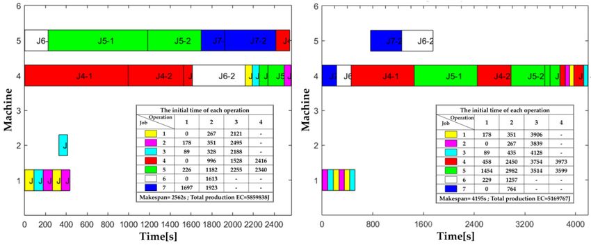
Sustainability 2019, 11, 179                                                                         2 of 21

      A machining system (MS), as a typical manufacturing system, usually comprises machine tools,
fixtures, cutting tools, workpieces, operators and various machining processes [3]. Since machines are
entities implementing various machining processes and the final products are usually directly or indirectly
processed by machines, machines are important energy consuming units in MS. Accordingly, reducing
the EC of machines has already been proved to be a significant strategy to improve manufacturing
sustainability [4]. In general, the energy-saving methods for MS follows two types, namely energy-efficient
process planning and energy-efficient scheduling [5]. The former mainly pays attention to the machining
EC of machines while the latter aims to minimize non-value added EC in manufacturing process.
However, the energy use breakdown in machining processes shows that actual material removal energy
is minimal compared with the energy used by auxiliary functions and components of a machine [6].
Furthermore, idle and loss EC take up more than 40% of total EC [7]. Hence, there is a greater energy-saving
potential from the manufacturing system-level perspective. As a workshop can be interpreted as a MS,
energy-efficient scheduling (ES) is easier to accept by manufacturing enterprises because it does not
substantially change the existing legacy system and requires less investment.
      Shop scheduling is a classical decision-making problem, and different scheduling problem types
can be categorized by the flowing types of workpiece in the workshop [8]. Owing to the lack of enough
attention to the environmental impact of MS in the past, ES research considering EC or environment
impact is rather limited and mainly aimed at single machine and flow shop modes. The job shop
mode is prevalent in small and medium enterprises, and flexible manufacturing mode is gradually
accepted by them for meeting diversified customers’ needs and responding to market changes rapidly.
Therefore, ES for flexible job shops is worth studying. Besides, traditional job shop scheduling (JSS)
and flexible job shop scheduling (FJSS) research usually ignored transportation time. As considering
transportation time will make the optimized shop floor schedule more practical, transportation time or
the influence of transport resources have already been taken into account in some FJSS research [9,10].
Yet, the effects of transportation factors on EC are not involved in these studies. In view of this,
considering transportation time, a new general ES model for flexible job shops with two performance
criteria, total production EC and makespan, is proposed in this paper.
      In the rest of this paper, a literature review on ES for various shop types and the motivation
for our research in Section 2 are followed by Section 3 describing the energy-efficient flexible job
shop scheduling (EFJSS) problem and the establishment of corresponding model. Details of the
application of the non-dominant sorting genetic algorithm-II (NSGA-II) for solving the presented
model is illustrated in Section 4, and verifying experiments and results are focused in Section 5.
Section 6 presents conclusions and prospects for future research.

2. Literature Review
     Since machines are key manufacturing resources as well as the main energy sources in a workshop,
ES is usually conducted to effectively manage machines from the EC perspective. In general, machine
state can be classified into four situations, i.e., start, machining, idle and stop. As ordinary machines
are usually operated and controlled manually, the operation time is of great uncertainty. So current
energy-efficient MS research mainly addresses numerical control (NC) machines, and the machining
EC of a machine can be calculated by the established machining process EC models and further viewed
as a constant when the process documents are given [11]. Hence, the EC of machines that current
ES research focuses on is different owing to various shop types. As the machining EC of a specific
machine often differs when various processing parameters are selected, a small amount of research
integrates processing parameter selection to reduce machining EC. By contrast, non-machining EC has
drawn significant attention in ES study from the shop-floor level.
     Regarding energy-efficient single machine scheduling (SMS), the most valuable achievement
is the proposal of energy-efficient mechanism, i.e., switching off the non-bottleneck idle machines
if no job needs it [12]. Beyond that, the existing related work mainly focused on the development
and/or improvement of dispatching rules, and the influence of different scheduling conditions on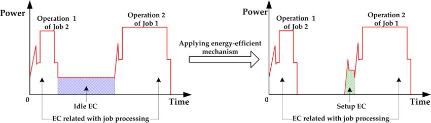
Sustainability 2019, 11, 179                                                                        3 of 21

optimization objectives [12–14]. For instance, as energy prices usually fluctuate, reducing EC can
not only reduce CO2 emissions but also save manufacturing costs, especially at the peak period of
electricity consumption or high energy price periods.
     The main reason for carrying out energy-efficient parallel machine scheduling (PMS) is that
the machines with the same manufacturing capability usually hold different energy efficiency.
Accordingly, some research considers processing parameter setting simultaneously. Fang et al. [15]
investigated minimizing the weighted sum of tardiness penalty and power consumption cost by
considering a higher cutting speed may enhance the productivity at the cost of more EC. Similarly, in view
of the fact that a higher cutting speed may incur high power load peaks, Wang et al. [16] examined the
PMS problem with flexible resources and a bounded power demand peak.
      Regarding energy-efficient flow shop scheduling (FSS) and the extension of it, different mixed
integer programming models considering EC and EC-related objectives (e.g., peak power, power
cost and carbon footprint) had been proposed under various conditions in the existing study [17–21].
Typically, Luo et al. [18] studied a hybrid FSS problem with the continuous change of electricity
price; in [20], not only the energy-efficient mechanism proposed in energy-efficient SMS research was
introduced into an energy-efficient flexible flow shop scheduling (FFSS) model but also spindle speed
selection was integrated; Wu et al. [21] established a FFSS model considering the periodicity and the
limited storage capacity of renewable energy.
      Regarding ES for a job shop, as each job has a fixed process route, total job-related processing EC
can be viewed as a constant and black box, and total idle EC attracts the most attention [22]. As for a
flexible job shop, although it is the extension of the job shop, the EC concerned is different. Since the
task-driven EC is greatly influenced by the variability and flexibility of task flow [23], EC can be
optimized by selecting suitable machines for jobs and arranging appropriate processing sequences in
flexible job shops [11]. Correspondingly, total production EC, including total processing EC and idle
EC, or total environmental impact according to the conversion relationship between energy and CO2
emissions, can be optimized [24].
      To summarize, ES research considering objectives related to environmental influence is increasing
but limited. Current study mostly focuses on SMS and FSS, and other shop types are seldom touched,
especially flexible job shop. However, the effectiveness of several typical energy-saving methods
stated in the aforementioned research has been verified, including operation sequencing, switching
off the idle machine and then switching on it before the arrival of new job (i.e., an energy-efficient
mechanism), process route selection, and machining parameter selection. Among them, process route
selection is not applicable for workshops in which each job has a fixed process route (e.g., classical
job shop) and machining parameter selection is only suitable for the condition that an operation has
alternative machining parameters. Moreover, EC calculation is the basis of EC optimization, resulting
in the application effect of the optimized scheduling schemes depending largely on the accuracy and
reliability of energy models or data of machines. Nevertheless, the real and reliable energy-related
data provided in the existing ES cases is rather limited, leading to enormous difficulty in evaluating
the energy-saving effect objectively. In contrast, more focus is on the algorithms for solving scheduling
problems, especially modern intelligent algorithms, such as genetic algorithm (GA), particle swarm
optimization (PSO) algorithm, Simulated annealing (SA) algorithm and the hybrid algorithm based on
them. Therefore, how to reduce EC through operational approaches has not been well investigated
for a typical flexible job shop environment, and a relatively general EFJSS model needs addressing
to facilitate the follow-up research with more sophisticate situations, e.g., machine failure, workload
constrains or recirculation. In addition, although some research had already been carried out on
the combination of energy-efficient mechanism with energy-efficient SMS, FFSS, and JSS [12,20,22],
how to apply energy-efficient mechanism to an EFJSS environment is a gap in the existing study, which
deserves exploring.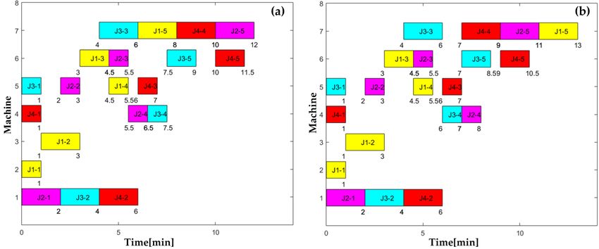
Sustainability 2019, 11, 179 4 of 21
3.Sustainability
Energy-Efficient
2019, 11, x Flexible
FOR PEER Job Shop Scheduling Model
REVIEW 4 of 22
Based
Based on
on previous
previous studies,
studies, manufacturing
manufacturing ECEC is
is tried
tried to
to be
be reduced
reduced by
by ES
ES combined
combinedwith
with
energy-efficient mechanism in flexible job shops. Correspondingly, EC and makespan, reflecting
energy-efficient mechanism in flexible job shops. Correspondingly, EC and makespan, reflecting
production
productionefficiency,
efficiency,are
arechosen
chosenasastwo
twooptimization
optimizationobjectives.
objectives.
3.1. Energy-Efficient Mechanism
3.1. Energy-Efficient Mechanism
When
Whenaamachine
machineisisturned
turned on, there
on, thereis aisstart-up
a start-uporder among
order amongdifferent power
different supply
power modules
supply (e.g.,
modules
power supplysupply
(e.g., power for electricity box, main
for electricity box,power
main supply, and power
power supply, andsupply
powerfor NC system).
supply for NC The power
system). Theoff
sequences are usually in the opposite order of the start-up. As these operations are
power off sequences are usually in the opposite order of the start-up. As these operations are usually usually regulated
inregulated
machine in manual,
machine themanual,
corresponding EC for a specific
the corresponding machine
EC for can be
a specific measured
machine canorbecalculated,
measuredthenor
viewed as a constant value. Hence, if the influence of warm-up operation after
calculated, then viewed as a constant value. Hence, if the influence of warm-up operation afterstarting up on machining
quality
startingisup
ignored, energy quality
on machining will be issaved by switching
ignored, energy willthebeidle machine
saved off and the
by switching then switching
idle machineitoffon
before a new
and then job arrives.
switching it on Such
beforea aturn-off
new joband then Such
arrives. turn-on operation
a turn-off andsequence was operation
then turn-on defined assequence
a “Setup”
operation in [12], and this definition is adopted in our study. Accordingly, energy-efficient
was defined as a “Setup” operation in [12], and this definition is adopted in our study. Accordingly, mechanism
isenergy-efficient
the execution of Setup operation,
mechanism as is displayed
is the execution of Setup byoperation,
Figure 1. as is displayed by Figure 1.
Figure 1.
Figure 1. The schematic diagram of
of the
the energy-efficient
energy-efficient mechanism.
mechanism.
When
Whenputting
puttingthis
thisenergy-efficient
energy-efficientmechanism
mechanismininpractical
practical use,
use,it is essential
it is to to
essential judge
judge whether
whether the
idle
the machines should
idle machines be off.be
should Based
off. on previous
Based analysis,analysis,
on previous a Setup operation takes at least
a Setup operation takesa predefined
at least a
predefined
amount amount
of time of ),
(TSetup time (TSetup
so the ), so the corresponding
corresponding EC (ESetupEC (ESetup
) can be )viewed
can be viewed as constant
as constant for a
for a specific
specific machine.
machine. Suppose Suppose
Tidle isTthe
idle is the inter-arrival
inter-arrival timetime between
between jobs,
jobs, since
since thetheidle
idlepower
power of aamachine
machine
(PSO
(P SO)) is
is usually stable, the
usually stable, the idle
idle EC EC isisthe productofofPPSOSOand
theproduct and Tidle
Tidle . Obviously,
. Obviously, whenwhenTidleT≥ T ≥ Tand
idleSetup Setup
SO
andSOP Tidle ≥ ESetup are both satisfied, amounts of energy can be saved as Setup operations can be
P Tidle ≥ ESetup are both satisfied, amounts of energy can be saved as Setup operations can be executed
executed during the idle periods. Let TB be the break-event duration, i.e., the least time required for a
during
Setup the idle periods.
operation, it can beLet TB be the
calculated by:break-event duration, i.e., the least time required for a Setup
operation, it can be calculated by:
ESetup
TB = ESetup (1)
TB = PSOSO (1)
P
Accordingly, if Tidle ≥ max( TB , TSetup ), the idle machine can perform Setup operation.
Accordingly, if Tidle ≥ max(TB , TSetup ) , the idle machine can perform Setup operation.
3.2. Problem Statement and Model Hypothesis
3.2. Problem Statement and Model Hypothesis
FJSS is further developed from classical JSS. To obtain feasible scheduling schemes, two subordinate
issues,FJSS
i.e., ismachine
further selection
developed and from classicalsequencing,
operation JSS. To obtain
needsfeasible
tackling.scheduling
Moreover, schemes, two
as EC is an
subordinate issues, i.e.,
environment-related machine
objective, it isselection and operation
vital to evaluate it whensequencing,
modeling aneeds tackling. Moreover, as EC
FJSS problem.
is anAlthough
environment-related
a MS contains objective,
variousit technical
is vital to equipments
evaluate it when modeling adifferent
and consumes FJSS problem.
types of energy
and media (e.g., electricity, diesel and cooling water), we only pay attention to the types
Although a MS contains various technical equipments and consumes different directof
ECenergy
of NC
and media
machines in (e.g., electricity,
the whole diesel andprocess,
manufacturing coolingandwater), we onlyEC
the indirect pay attention
[25] to the
as well as the embodied
direct EC EC
of NC
[26]
machines in the whole manufacturing process, and the indirect EC [25] as well as the
of auxiliary materials is ignored in order to simplify study and facilitate result comparison. Based on embodied EC
[26] of auxiliary
current research,materials
some otheris ignored in order
assumptions to simplify
made study and
for modeling facilitate
EFJSS result
are listed comparison. Based
below.
on current research, some other assumptions made for modeling EFJSS are listed below.
(1) Jobs are mutually independent and there is no priority difference for them.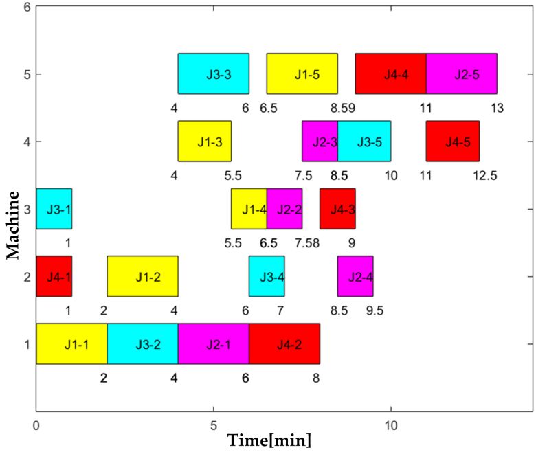
Sustainability 2019, 11, 179                                                                             5 of 21

(1)  Jobs are mutually independent and there is no priority difference for them.
(2)  Each machine cannot process more than one job at a time, and job pre-emption or cancellation is
     forbidden once processing starts.
(3) Each job contains sequential operations, and each operation can only be executed on one machine
     in actual production. When an operation of a job, not the terminal operation, ends, such a job is
     immediately transported to the machine arranged for its next operation, i.e., without regard for
     batch transportation.
(4) Transportation time varies with the different machines selected for pre- and post-operation
     of a job, and it is only related to transportation distance. In particular, transportation time is
     considered as zero under the condition that a machine processes two adjacent operations of a job.
(5) Input buffer of each machine is unlimited. The initial position of each job is the machine
     executing its first operation, and the ending position is the machine performing its last operation,
     i.e., transportation is not needed for the first and the last operations of each job.
(6) The processing time of an operation is composed of machining time and auxiliary time (e.g.,
     clamping, inspection and cleaning times).
(7) Each operation on the selected NC machine is executed according to the fixed NC programs.
(8) All jobs are simultaneously available at time zero, and breakdown is not considered.
(9) Total production EC is evaluated with makespan as time boundary.
(10) The energy-efficient mechanism is adopted, and the warm-up operation is neglected.

3.3. Mathematical Model
      A typical EFJSS problem contains m machines and n jobs. Each job i (i = 1, 2, . . . , n) comprises
a sequence of operation Oij , j = 1, 2, . . . , Ji , where Ji represents the total number of operations in
job i. All operations that can be executed on machine k (k = 1, 2, . . . , m) form a set Nk , and each
operation Oij in Nk has a corresponding processing time and EC, denoted as TPijk and MEijk respectively.
According to the Therblig-based energy supply models of machines, the idle power of machine k can
be identified by its Therblig-SO power, namely PkSO . The Setup operation time and the corresponding
                                    Setup         Setup
EC of machine k is denoted as Tk           and Ek        respectively. TRTkq is the transportation time from
machine q (q = 1, 2, . . . , m) to machine k. H is an extremely large positive number. In addition, some
decision variables, namely Sij , Cij , Xijk and Yiji∗ j∗ k , are denoted, where Sij and Cij indicate the initial
and terminal time of Oij respectively, Xijk is an integer variable whose value is 1 if machine k executes
Oij and 0 otherwise, and Yiji∗ j∗ k is also an integer variable with value 1 if Oij is processed before Oi∗ j∗
when they are both executed on machine k and 0 otherwise.
     As the time boundary for analyzing EC, the makespan of all jobs (Tmakespan ) can be obtained by:

                                         Tmakespan = max Cij , ∀i, j                                        (2)

      Consequently, the total production EC (Etotal ) is the sum of the EC of all machines related with
jobs, which can be expressed below:
                                                        m
                                            Etotal =   ∑ (EIk + EMk )                                       (3)
                                                       k =1

where EIk is the sum of EC during all standby periods of machine k and EMk is the total processing EC,
which can be further presented below:

                                      EMk =            ∑            MEijk Xijk , ∀k                         (4)
                                                {(i,j):Oij ∈ Nk }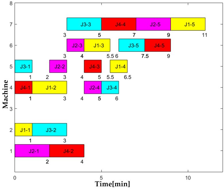
Sustainability 2019, 11, 179 6 of 21
As for EIk , when all machines are not allowed to be turned off during idle time, it can be expressed as:
EIk = PkSO max
{(i,j):Oij ∈ Nk }
{Cij } − min
{(i,j):Oij ∈ Nk }
{Sij } − ∑ TPijk Xijk , ∀k (5)
{(i,j):Oij ∈ Nk }
For a given scheduling scheme, the machine distribution for each operation is determined. Let Rk
be the actual number of operations executed on machine k, which can be calculated by:
Rk = ∑ Xijk , ∀k (6)
{(i,j):Oij ∈ Nk }
Obviously, if there are Rk operations processed on machine k, Rk −1 idle intervals between adjacent
operations will exist at most. Suppose Oij is the lth (1 ≤ l ≤ Rk −1) operation performed on machine k,
Oi0 j0 is its adjacent subsequent operation on machine k, and the parameters, namely Sij , Cij , Si0 j0 and
( l +1) k ( l +1) k
Ci0 j0 , are remarked as Sijlk ,Cijlk ,Si0 j0 and Ci0 j0 respectively, the EC of each idle interval on machine k
when applying an energy-efficient mechanism can be expressed as follows:
ESetup ( l +1) k
if PkSO (Si0 j0 − Cijlk ) > Ek
Setup
and (Si0 j0
( l +1) k Setup
− Cijlk ) > Tk
k
EIkl = ,
PSO (S(0l +0 1)k − C lk ) otherwise (7)
k ij ij
∀k, (i, j), (i0 , j0 ) : Oij ∈ Nk , Oi0 j0 ∈ Nk , Xijk = 1, Xi0 j0 k = 1, Yiji0 j0 k = 1; l = 1, 2, . . . , Rk − 1
Then, EIk can be presented below:
R k −1
EIk = ∑ EIkl (8)
l =1
According to Formulae (5)–(7), no matter whether the energy-efficient mechanism is applied, EIk
is mainly determined by the decision variable Sij , Cij and Xijk . Combined with Formula (4), it can be
known that the EC calculation is closely related to the values of decision variables. So it is essential to
acquire the values of all decision variables firstly to further calculate EC. The optimization objectives
are presented below: (
Minimize[ Tmakespan ]
(9)
Minimize[ Etotal ]
subject to:
∑ Xijk = 1, (10)
k:Oij ∈ Nk
Cij = Sij + ∑ TPijk Xijk , ∀i, j (11)
{k:Oij ∈ Nk }
Cij − Ci∗ j∗ + H (1 − Xijk ) + H (1 − Xi∗ j∗ k ) + HYiji∗ j∗ k ≥ TPijk , ∀k, (i, j), (i∗ , j∗ ) : Oij , Oi∗ j∗ ∈ Nk (12)
Ci∗ j∗ − Cij + H (1 − Xijk ) + H (1 − Xi∗ j∗ k ) + H (1 − Yiji∗ j∗ k ) ≥ TPi∗ j∗ k , ∀k, (i, j), (i∗ , j∗ ) : Oij , Oi∗ j∗ ∈ Nk (13)
H (1 − Xijk ) + H (1 − Xi( j−1)q ) + Sij − Ci( j−1) ≥ TRTkq , ∀k, q, i, j = 2, . . . , Ji : Oij ∈ Nk , Oi( j−1) ∈ Nq (14)
Sij ≥ 0, ∀i, j (15)
Constraint (10) represents that each operation is not allowed to be executed on more than one
machine anytime. Constraint (11) notes that machine selection affects the earliest finish time of an
operation, and the processing cannot be interrupted until it is finished. Constraints (12) and (13) are
to guarantee that two operations belonging to various jobs cannot be executed simultaneously when
both are arranged on the same machine. Constraint (14) states that precedence relationships cannotSustainability 2019, 11, 179 7 of 21
Sustainability 2019, 11, x FOR PEER REVIEW 7 of 22
be violated
be violated and
and transportation affects the
transportation affects the initial
initial time
time of
of each
each operation.
operation. Constraint (15) ensures
Constraint (15) ensures that
that
the initial time of each operation is non-negative. Furthermore, it can be concluded that the
the initial time of each operation is non-negative. Furthermore, it can be concluded that the allowableallowable
earliest initial
earliest initial time
time of
of an
an operation
operation is
is constrained
constrained by by transportation
transportation and
and manufacturing
manufacturing resource
resource from
from
Constraints (12)–(14), and such an impact relationship can be depicted by
Constraints (12)–(14), and such an impact relationship can be depicted by Figure 2.Figure 2.
2. Constraints
Figure 2. Constraintsofof
transportation timetime
transportation and equipment resources
and equipment on the starting
resources on the time of antime
starting operation.
of an
operation. setup setup
When calculating Etotal , the input parameters, namely TPijk , MEijk , PkSO , Tk , Ek and TRTkq ,
should be obtained in advance. The processing time of an operation (TP
When calculating Etotal, the input parameters, namely TPijk, MEijk, Pk ijk , Tk SO ) consists
setup of
setup machining
, Ek and TRTkq,
time and necessary auxiliary time based on a research assumption. Since the NC program contains
should be obtained in advance. The processing time of an operation (TPijk) consists of machining time
the information of cutting tool path and processing parameters, machining time can be obtained
and necessary auxiliary time based on a research assumption. Since the NC program contains the
by analyzing the NC program [27]. Besides, in order to make reasonable production plans and
information of cutting tool path and processing parameters, machining time can be obtained by
analyze production efficiency, the standard labor time or man-hour quota is commonly applied in
analyzing the NC program [27]. Besides, in order to make reasonable production plans and analyze
manufacturing enterprises. Correspondingly, the auxiliary time of each operation can be viewed as a
production efficiency, the standard labor time or man-hour quota is commonly applied in
constant. Except process time analysis, the EC models of related machines also need to be established
manufacturing enterprises. Correspondingly, the auxiliary time of each operation can be viewed as
beforehand. Although a multitude of research has been carried out on EC modeling for machines
a constant. Except process time analysis, the EC models of related machines also need to be
and various models has been put forward, the Therblig-based model [28,29] is adopted here in view
established beforehand. Although a multitude of research has been carried out on EC modeling for
of accuracy and applicability. Furthermore, MEijk can be calculated by combining the analysis of
machines and various models has been put forward, the Therblig-based model [28,29] is adopted
processing time with the already Therblig power models of machines, including Therblig-SO power
here in view of accuracy and applicability. Furthermore,
setup MEijk can be calculated by combining the
(PkSO ). In addition, the Setup operation time (Tk ) can also be obtained by the methods of making
analysis of processing time with the already Therblig setup power models of machines, including Therblig-
standard laborSOtime, and the corresponding EC (Ek ) can be measured with EC collection equipment.
setup
SO power ( Pk ). In addition, the Setup operation time ( Tk ) can also be obtained by the methods
Moreover, due to the relatively fixed workshop layout and the assumption that transportation time is
of making
only relatedstandard labor time,distance,
to transportation and the the
corresponding
transportation ( Eksetup
EC time ) can bevarious
between measured with EC(TRT
machines collection
kq ) can
be set by a man-hour quota system or obtained through simulation with some
equipment. Moreover, due to the relatively fixed workshop layout and the assumption that digital plant simulation
softwares (e.g., Delmia
transportation time is Quest and Tecnomatix).
only related to transportation distance, the transportation time between
various machines (TRTkq) can be set by a man-hour quota system or obtained through simulation with
4. Model Solution Based on Non-Dominated Sorting Genetic Algorithm-II(NSGA-II)
some digital plant simulation softwares (e.g., Delmia Quest and Tecnomatix).
FJSS is NP-hard and it is formidable to obtain the exact optimal solutions for large scale problems
4. Model Solution
in finite time. Hence, Based on intelligent
modern Non-Dominated Sorting
algorithms, e.g.,Genetic
ant colony Algorithm-II(NSGA-II)
optimization (ACO) algorithm, GA,
PSO and SA, are gradually prevalent, and have been utilized for
FJSS is NP-hard and it is formidable to obtain the exact optimal solutions seeking the near-optimal solutions
for large scale of a
problems
FJSS problem in reasonable time [30,31]. Furthermore, the established EFJSS model
in finite time. Hence, modern intelligent algorithms, e.g., ant colony optimization (ACO) algorithm, is a multi-objective
function
GA, PSOwith andconstraints. Obviously,
SA, are gradually the solution
prevalent, andofhave
it is actually solving for
been utilized a multi-objective optimization
seeking the near-optimal
problem (MOP). However, it is impossible to make all independent and conflicting
solutions of a FJSS problem in reasonable time [30,31]. Furthermore, the established EFJSS model objectives optimal
is a
simultaneously. Traditional basic idea for solving an MOP is transforming it
multi-objective function with constraints. Obviously, the solution of it is actually solving a multi- to a single-objective
optimization
objective problem (SOP),
optimization problem and (MOP).
the typical methodsit include
However, the weighted
is impossible to make sum, allgoal programming
independent and
conflicting objectives optimal simultaneously. Traditional basic idea for solving anInMOP
and min-max algorithm [32,33]. However, the solution of a MOP is usually not unique. view ofis
the advantages of the intelligent optimization algorithm, namely high parallelism,
transforming it to a single-objective optimization problem (SOP), and the typical methods include self-organization,
self-learning
the weighted and sum,self adaptation,
goal programming the NSGA-II originated
and min-max from GA
algorithm is utilized
[32,33]. However,to acquire the Pareto
the solution of a
set of the proposed EFJSS model. The general flow chart of NSGA-II is shown
MOP is usually not unique. In view of the advantages of the intelligent optimization algorithm, by Figure 3, and more
details can
namely high beparallelism,
known fromself-organization,
[34]. self-learning and self adaptation, the NSGA-II originated
from GA is utilized to acquire the Pareto set of the proposed EFJSS model. The general flow chart of
NSGA-II is shown by Figure 3, and more details can be known from [34].Sustainability 2019, 11, 179 8 of 21
Sustainability 2019, 11, x FOR PEER REVIEW 8 of 22
Figure 3. The flow chart of the non-dominated sorting genetic algorithm-II(NSGA-II)
4.1. Encoding Scheme
4.1. Encoding Scheme
FJSS
FJSS need
need address
address two two core
core issues: machine selection
issues: machine selection and and operation
operation sequencing.
sequencing.
Correspondingly,
Correspondingly, the
the chromosome
chromosome shouldshould contain
contain thethe information
information related
related to to machines and operation
machines and operation
sequences, and the operation-based encoding schema can be adopted. Each
sequences, and the operation-based encoding schema can be adopted. Each gene in a chromosome gene in a chromosome
representing an operation
representing an operation isiscoded
codedas asthe form(i,(i,k).k).The
theform Thejthjth gene
gene likelike k) k)
(i, (i, stands
stands OijO
forfor ij executed
executed on
on machine k. Moreover, the genes related to job i should appear J times, and they
machine k. Moreover, the genes related to job i should appear Ji times, and they are located in the
i are located in the
chromosome
chromosome randomly
randomly while
while satisfying
satisfying order
order constraints. Therefore, the
constraints. Therefore, chromosome length
the chromosome length of each
of each
n
individual representing a solution is ∑n
Ji .
individual representing a solution is i
=1 J i .
i =1
4.2. Decoding Scheme
4.2. Decoding Scheme
The evaluation of each objective relies on the values of decision variables when all input parameters
The evaluation
are known. of eachchromosome
Correspondingly, objective relies
decodingon isthe values
mainly of decision
to determine the variables when all
values of decision input
variables
parameters are known. Correspondingly, chromosome decoding is mainly to determine
which actually reflect the machine selection and time information of each job, obtaining feasible schedule the values
of decision
and variables
the values which actually
of optimization reflectAccording
objectives. the machine selectionhypotheses,
to research and time information of each
there are three job,
possible
obtainingtypes,
schedule feasible schedule
namely and the
semi-active valuesactive
schedule, of optimization objectives. schedule
schedule and non-delay According[35].toIn research
order to
reduce total production EC as much as possible while shortening makespan, the active schedule isschedule
hypotheses, there are three possible schedule types, namely semi-active schedule, active adopted
and
in ournon-delay
study, andschedule
a decoding[35]. In order
method basedtoonreduce total production
[36] is presented to acquireEC as much
feasible asschedule
active possibleand while
the
shortening makespan, the active schedule is adopted in our study, and a decoding method
corresponding values of other decision variables. Suppose ASij is the allowable earliest starting time of O based on,
ij
[36] is presented to acquire feasible active schedule
the decoding details for any given chromosome are expressed below:and the corresponding values of other decision
variables. Suppose ASij is the allowable earliest starting time of Oij, the decoding details for any given
Step 1 Acquire
chromosome arethe Xijk and Yiji∗ j∗ k by Constraint (10) and the encoding schema.
values ofbelow:
expressed
Analyze the genes successively, and determine the value of Sij . For the gene (i, k) representing Oij , ASij
Step 1 isAcquire
non-negative, and AS
the values ofij X=ijkCand
i ( j−1)Y+* TRT based on Constraints
bykqConstraint (10) and the and (15), ∀i,
(14) encoding j = 2, 3, . . . , Ji , k,
schema.
iji j * k
q:Oij ∈ Nk , Oi( j−1) ∈ Nq . Check the operations performed on machine k that have already been
Step 2 analyzed
Analyzeand theobtain
genes successively,
all idle ranges [IT_S, and determine
IT_E]. Then, check theeach value
idle of Sij. For
interval the
[IT_S, IT_E]gene (i, k)
Step 2 = Cand + TRTkq of
representing
successively, Oij, ASijij, is
if max{AS non-negative,
IT_S} + TPijk ≤ IT_E, Sij AS
and = IT_S
ij i ( j −1)the value
based
related onYiji
Constraints (14)
∗ j∗ k should be
changed according to new order; otherwise, check next idle range.
and (15), ∀i , j = 2, 3, ..., Ji , k, q: Oij ∈ Nk , Oi ( j −1) ∈ Nq . Check the operations When O ij cannot be inserted
performed on into
any idle range, Sij will take the maximum of ASij and the end time of the immediate predecessor of Oij
onmachine
machinekkthat have already
according to Constraint been(12) analyzed and(13).
along with obtain all idle ranges [IT_S, IT_E]. Then,
Determine the value of Cij . According to Constraint (11), Cif
check each idle interval [IT_S, IT_E] successively, max{ASij, IT_S}+TPijk≤IT_E, Sij=IT_S
ij = Sij + TPijk . If the genetic analysis is not
Step 3
and theturn
finished, value of related
to Step 2. Yiji* j* k should be changed according to new order; otherwise,
Combined with the obtained values of decision variables, Tmakespan can be determined by Formula (2)
Step 4 check next idle range. When Oij cannot be inserted into any idle range, Sij will take the
and Etotal can be calculated by Formulae (3) and (4), (6)–(8).
maximum of ASij and the end time of the immediate predecessor of Oij on machine k
according to Constraint (12) along with (13).
Step 3 Determine the value of Cij. According to Constraint (11), Cij=Sij+TPijk. If the genetic analysis
is not finished, turn to Step 2.Sustainability 2019, 11, 179 9 of 21
4.3. Initial Population
Based on the encoding schema, a set including all values of job layer can be obtained firstly, i.e.,
n
there are Ji elements equal to i, and the number of all elements in such set is ∑ Ji . Then, owing to the
i =1
n
fixed chromosome length (i.e., ∑ Ji ), all elements will be randomly assigned to the job layer of each
i =1
gene in the chromosome. Correspondingly, the operation represented by each gene can be acquired.
Finally, assign a machine to each operation from its optional machine set randomly, acquiring the
value of the corresponding gene’s machine layer.
4.4. Non-Dominated Sorting
All feasible solutions can be represented by different individuals of the population, and they can
be ranked in various Pareto fronts through non-dominated sorting. The objective functions shown by
Formulae (2) and (3) are used to evaluate the dominance relationship between different individuals,
then determining the fronts as well as its containing elements. Correspondingly, the individuals
belonging to higher front set are preferable. The commonly-used method for non-dominated sorting is
fast sort algorithm, which had been fully illustrated in [34].
4.5. Crowding Distance Sorting
The introduction of crowding distance is to assess the Euclidian distance between individuals
belonging to the same front according to their objective values. Accordingly, crowding distance
sorting can guarantee the diversity of population, which is similar to genetic mutation operation.
Note that crowding distance comparison is meaningless for individuals with various Pareto ranks.
Generally, the crowding distance for an individual locating between two boundaries of the front is
the sum of the normalized distance between its adjacent neighbors based on each objective function.
In particular, the crowding distances for individuals distributed in the boundary are set to infinity.
4.6. Genetic Operators
Selection is carried out based on tournament selection here. Firstly, select a certain number of
individuals from the current generation randomly. Then, make non-dominated sorting and crowding
distance sorting based on the decoded objective function values. The individual locating in a higher front
as well as having the largest crowding distance will be selected to form a mating pool, whose size is usually
set as half of the population size. Such operations will be repeated until the mating pool is full, and the
following crossover and mutation operations will be carried out based on the individuals in mating pool.
Regarding crossover operation, a single-point crossover operator is applied. The detailed
procedures and a crossover example for 3 × 3 flexible job shop are shown by Figure 4.
Then the swap mutation operator, i.e., exchanging two different arbitrary genes of the
chromosome, is employed for a mutation operation. In particular, if such two genes having the
same value on job layer, the chromosome obtained after mutation operation may be illegal, as each
gene represents an operation and the contents of each operation’s alternative machine set are usually
various. Hence, it is necessary to further examine the values of machine layer for two swapped genes
in this condition. If the machine selected cannot execute an operation, choose a machine from its
alternative machine set randomly, then update the value of machine layer for the corresponding gene.Sustainability 2019, 11, 179 10 of 21
Sustainability 2019, 11, x FOR PEER REVIEW 10 of 22
Figure 4. Single-point crossover operation and an example.
5. Experiments
5. Experiments
To evaluatethe
To evaluate therelationship
relationship of two
of two criteria
criteria in flexible
in flexible job apply
job shops, shops,theapply the improved
proposed proposed
improved scheduling approach and verify the effectiveness of NSGA-II in solving
scheduling approach and verify the effectiveness of NSGA-II in solving a EFJSS problem, a EFJSS problem,
two
two experiments
experiments werewere conducted
conducted respectively.
respectively.
5.1. Experiment 1
5.1. Experiment 1
Owing to the lack of FJSS examples with reliable EC data in the current study, this experiment
Owing to the lack of FJSS examples with reliable EC data in the current study, this experiment
was carried out based on the example in our early study [37], and the EC data needed was further
was carried out based on the example in our early study [37], and the EC data needed was further
enriched. Such an example was composed of five machines and seven independent jobs corresponding
enriched. Such an example was composed of five machines and seven independent jobs
to three sorts of parts, as shown in Figure 5. Moreover, the established Therblig power models of each
corresponding to three sorts of parts, as shown in Figure 5. Moreover, the established Therblig power
machine, the detailed process plan of each job, as well as the EC calculation for each operation can
models of each machine, the detailed process plan of each job, as well as the EC calculation for each
also be referred
operation to. Some
can also important
be referred information,
to. Some including
important TPijk and
information, MEijk , isTP
including briefly shown in Table 1.
ijk and MEijk, is briefly
setup setup
Additionally, to determine Ek and Tk , the experimental
Eksetup and Tsetup setup used for Therblig power modeling
shown in Table 1. Additionally, to determine k
, the experimental setup used for
can still be applied according to the standard operation specification of each machine, and an example
Therblig power modeling can still be applied according to the standard operation specification of
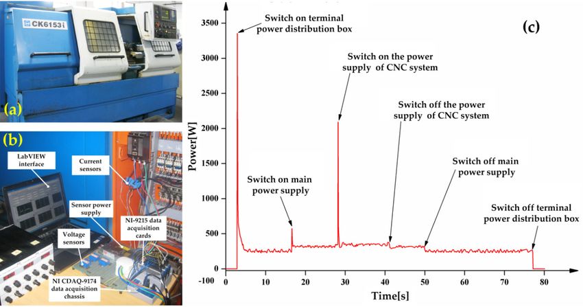
is displayed in Figure 6. The Setup operation was carried out by skilled workers three times for each
each machine, and an example is displayed in Figure 6. The Setup operation was carried
setup setupout by skilled
machine, and the mean values of the measured EC and time were set as Ek and T respectively,
workers three times for each machine, and the mean values of the measured EC andk time were set as
as expressed in Table 2. Besides, the virtual environment of manufacturing workshop was established
Eksetup Delmia
with k
setup
and TQuest. respectively,
All workpieces as were
expressed
transported in Table 2. Besides,
by handcart, the
then thevirtual
average environment
transportation of
manufacturing
time workshop
between different was established
machine tools (i.e., TRTwith kq ) Delmia Quest. All
can be obtained workpieces
through logisticwere transported
simulation by
analysis,
handcart, then
as shown in Table 3. the average transportation time between different machine tools (i.e., TRT kq) can be
obtained through
Then, logistic simulation
the relationship betweenanalysis,
EC andasmakespan shown in Table 3.
was analyzed in four working modes.
Then, the
The former tworelationship
modes werebetween EC and
corresponding to makespan
EFJSS while wastheanalyzed in fourwere
rest two modes working modes. The
corresponding to
former two modes
energy-efficient were scheduling
job shop corresponding(EJSS).to However,
EFJSS while thethe rest two
difference modesinwere
existing corresponding
the former two modes to
energy-efficient
as well as the latter jobtwo
shop scheduling
ones (EJSS).
were the same, i.e.,However,
whether the theenergy-efficient
difference existing in the was
mechanism former two
applied.
modes as well
Specifically, an as the latter two mechanism
energy-efficient ones were the was same,
utilizedi.e., in
whether
modes the 1 andenergy-efficient
3. Note that the mechanism
arrangementswas
applied.
in mode 3Specifically,
and 4 shown anby
energy-efficient
Table 4 was mainly mechanism was utilized
for the balanced use ofin machines.
modes 1 and 3. Note that the
arrangements
After all in mode
input 3 and 4 shown
parameters neededby Table 4 was mainly
for evaluating Etotalfor the balanced
were determined,use ofthemachines.
NSGA-II was
After all input parameters needed for evaluating
implemented in Matlab language on a PC with Intel Core(TM) i5-6500 3.20GHz CPU, E total were determined, the NSGA-II
8GB RAM, was
implemented
and Windowsin7.Matlab language
The basic on a PC with
parameters Intel Core(TM)
for NSGA-II are listed i5-6500 3.20GHz
in Table 5. CPU,
Then,8GB the RAM, and
algorithm
Windows
was 7. The respectively
run 15times basic parameters for NSGA-II
to obtain the Pareto arefront
listedcorresponding
in Table 5. Then, the algorithm
to various workingwas run
modes.
15times respectively
Comparison of solutionsto obtain the working
in four Pareto front modescorresponding
is shown by toFigure
various7.working modes.
Specifically, Comparison
schedule Gantt
of solutions
charts in four working
corresponding modes inis two
to the solutions shown by Figure
boundaries of the7. Specifically,
Pareto front in schedule
workingGantt modecharts
1 are
corresponding
depicted by Figure to the
8. solutions in two boundaries of the Pareto front in working mode 1 are depicted
by Figure 8.Sustainability 2019, 11, 179 11 of 21
Table 1. Processing time and energy consumption (EC) of each operation [37].
Machine 1 2 3 4 5
Part Job
Operation (CK6136i) (CK6153i) (CAK6150Di) (JTVM6540) (XHK-714F)
89 s, 89 s, 89 s,
1 - -
1.0684 × 10⁵ J 1.2173 × 10⁵ J 1.2599 × 10⁵ J
84 s, 84 s, 84 s,
A 1–3 2 - -
0.8870 × 10⁵ J 1.0206 × 10⁵ J 1.0615 × 10⁵ J
67 s, 66 s,
3 - - -
4.7815 × 10⁴ J 4.7912 × 10⁴ J
996 s, 956 s,
1 - - -
1.0986 × 10⁶ J 1.1109 × 10⁶ J
532 s, 525 s,
2 - - -
5.3333 × 10⁵ J 5.4448 × 10⁵ J
B 4, 5
85 s,
3 - - - -
5.1481 × 10⁴ J
155 s, 133 s,
4 - - -
1.1115 × 10⁵ J 9.9921 × 10⁴ J
229 s, 226 s,
1 - - -
2.4488 × 10⁵ J 2.6095 × 10⁵ J
C 6, 7
508 s, 493 s,
2 - - -
5.1276 × 10⁵ J 4.8041 × 10⁵ J
Table 2. Average Setup operation time and EC of each machine.
Setup Setup
Machine k Ek [J] Tk [s] PSO
k [W]
CK6136i 1 1.9065 × 10⁴ 60 335.7
CK6153i 2 2.7800 × 10⁴ 75 332.1
CAK6150Di 3 2.8400 × 10⁴ 80 414.0
JTVM6540 4 2.7000 × 10⁴ 65 360.5
XHK-714F 5 2.9700 × 10⁴ 75 371.0
Table 3. Average transportation time of workpieces between different machines.
Target Position
CK6136i CK6153i CAK6150Di JTVM6540 XHK-714F
Initial Position
CK6136i 0 150 s 210 s 465 s 515 s
CK6153i 180 s 0 250 s 450 s 475 s
CAK6150Di 220 s 270 s 0 435 s 425 s
JTVM6540 485 s 460 s 500 s 0 535 s
XHK-714F 530 s 510 s 520 s 505 s 0
Table 4. Machine selection for each job in working mode 3 and 4.
Operation
1 2 3 4
Job
1 CK6136i CK6153i JTVM6540 -
2 CK6153i CAK6150Di XHK-714F -
3 CAK6150Di CK6136i JTVM6540 -
4 JTVM6540 XHK-714F JTVM6540 JTVM6540
5 XHK-714F JTVM6540 JTVM6540 XHK-714F
6 JTVM6540 XHK-714F - -
7 XHK-714F JTVM6540 - -
Table 5. Parameter setting of NSGA-II.
Population Evolutional Crossover Mutation Tournament
Parameter
Size Generation Probability Probability Size
Value 50 300 0.9 0.1 2Sustainability 2019, 11, 179 12 of 21
Sustainability 2019,
Sustainability 2019, 11,
11, xx FOR
FOR PEER
PEER REVIEW
REVIEW 12 of
12 of 22
22
Figure 5.
Figure
Figure 5. Three
5. Three kinds
Three kinds of
kinds of parts
of parts [37].
parts [37].
[37].
Figure6.
Figure 6.An
Anexample
exampleofofmeasuring
measuringSetup
Setupoperation
operationtime
operation timeand
andEC:
EC:(a)
(a)numerical
numericalcontrol
controllathe
latheCK6153i;
CK6153i;
(b)experimental
(b) experimentalsetup
setupfor
forEC
for ECdata
EC dataacquisition;
data acquisition;(c)
acquisition; (c)the
(c) thepower
the powerprofile
power profileof
profile ofSetup
of Setupoperation
Setup operationfor
operation forCK6153i.
for CK6153i.
CK6153i.Sustainability 2019, 11, 179
x FOR PEER REVIEW 13 of 21
22
Sustainability 2019, 11, x FOR PEER REVIEW 13 of 22
Figure 7.Solution comparison of four working modes.
Figure 7. Solution comparison of four working modes.
Figure 7.Solution comparison of four working modes.
Figure 8. Schedule
Figure 8. Schedule Gantt
Gantt charts
chartscorresponding
correspondingtotothe
thesolutions
solutionsinintwo
twoboundaries
boundariesofof
thethe
Pareto front
Pareto in
front
Figure
working 8. Schedule
mode 1.
in working mode 1. Gantt charts corresponding to the solutions in two boundaries of the Pareto front
in working mode 1.
As revealed by Figure 7, makespan conflicts with EC in the Pareto front in the first two working
As revealed by Figure 7, makespan conflicts with EC in the Pareto front in the first two working
modes.As When total production
revealed by Figure 7,EC was reduced
makespan by 11.7% fromin 5,859,838J to 5,169,797J, the corresponding
modes. When total production EC wasconflicts
reduced withbyEC 11.7% thefrom
Pareto front in the
5,859,838J to first two working
5,169,797J, the
makespan
modes. increased
When by
total 63.8%
productionfrom 2562
EC s to
was 4195 s. In
reduced the byPareto
11.7% front,
fromeven though
5,859,838J there
to was the same
5,169,797J, the
corresponding makespan increased by 63.8% from 2562 s to 4195 s. In the Pareto front, even though
change of makespan,
corresponding the degree
makespan of EC optimization
increased by 63.8% was2562
from quites todifferent.
4195 s. Hence,
In the makespan
Pareto andeven
front, EC can be
though
there was the same change of makespan, the degree of EC optimization was quite different. Hence,
treated as two
there was theindependent
same change optimization
of makespan, objectives
the degreein a of
flexible job shop environment.
EC optimization was quite AlthoughHence,
different. there
makespan and EC can be treated as two independent optimization objectives in a flexible job shop
were some regions
makespan and ECwhere
canthebe Pareto
treated fronts
as twowere very close oroptimization
independent coincide for working
objectivesmode in 1aclose
and 2, thejob
flexible region
shop
environment. Although there were some regions where the Pareto fronts were very or coincide
where the ParetoAlthough
environment. front obtainedthere inwere
workingsome mode 1 outside
regions where that
theinPareto
working mode
fronts 2 was
were veryrather large,
close or which
coincide
for working mode 1 and 2, the region where the Pareto front obtained in working mode 1 outside
means
for in an energy-efficient
working mode 1 and mechanism
2, therather further
region whereenhances
the Paretothe EC optimization
obtained potential on mode
the basis of ES.
that working mode 2 was large, which meansfront an energy-efficient in working
mechanism 1further
outside
According to Figuremode
that in working 8, the machine
2 was with higher
rather large, energy efficiency antended to be selected for an operation
enhances the EC optimization potential on the which
basis ofmeansES. According energy-efficient
to Figure 8,mechanism
the machinefurther with
when much
enhances more attention
the efficiency
EC optimization was paid to EC than makespan. However, the processing 8, the of
time Part B was
higher energy tended potential
to be selectedon theforbasis of ES. According
an operation when much to Figure
more attention machine
was paidwith
far longerenergy
higher than that of the other
efficiency tendedtwoto kinds
be of parts, for
selected so the
an completion
operation time of
when Part B
much determined
more attention makespan
was paid
to EC than makespan. However, the processing time of Part B was far longer than that of the other
totoa EC
large extent.
than Owing to
makespan. the smallthe
However, scale of example,
processing time the ofoverall
Part B solution
was far space
longer was
than relatively
that of limited
the other
two kinds of parts, so the completion time of Part B determined makespan to a large extent. Owing
totwo
thekinds
smallofscale
parts, ofsoexample,
the completion time solution
the overall of Part Bspace
determined makespan
was relatively to a large
limited andextent. Owing
the optimal
to the small scale of example, the overall solution space was relatively limited and the optimalSustainability 2019, 11, 179 14 of 21
and the optimal solution found in working mode 4 was unique. The solution comparison of working
mode 3 and 4 showed that total production EC could be further reduced by employing the energy-efficient
mechanism despite the same makespan (2826 s), which was consistent with the research conclusions in [22].
Meanwhile, the solution comparison between working mode 1 and 3 demonstrated that the flexibility of
machine selection can improve energy-saving potential obviously.
5.2. Experiment 2
This experiment was carried out from two aspects to evaluate the performance of the NSGA-II applied
in our study by comparing the solutions obtained with other intelligent algorithms. Firstly, the example in
Experiment 1 corresponding to the first working mode was solved with ACO used in [38]. Furthermore, By
reviewing the existing literature related to EFJSS, the example including four jobs and seven machines
in [39] was selected, and the performance comparison was made between the algorithms used in [39],
namely modified genetic algorithm (MGA) and GA-PSO, and the NSGA-II we used.
As a typical stochastic intelligent search algorithm, ACO is inspired by the behavior of ants
searching the shortest path during foraging. For a specific FJSS example, the number of total operations
is fixed, and each operation can be regarded as a node through which ants crawl. In each node,
the probability of a machine to be selected is affected by pheromone level and heuristic information.
Correspondingly, each ant constructs a solution to the scheduling problem by traveling all nodes.
Note that the precedence relationship of operations belonging to the same job results in the order of ants
passing through these nodes cannot be violated. The general idea of ACO in [38] was applying different
pheromone trail matrices for different optimization objectives. The iteration number, the number
of ants, the pheromone exponential weight, the heuristic exponential weight, and the pheromone
evaporation rate were assigned 300, 50, 2, 3 and 0.01 respectively in this ACO. For more details, such
as the probability distribution for node selection and the pheromone evaporation rule, can refer to [38].
Since the crawling path of each ant represents a solution to the problem, the operation-based encoding
scheme, the decoding scheme as well as the non-dominated sorting in this paper can all be used for
reference. In each iteration, only the ants in the non-dominated front were allowed to update both
pheromone matrices. Correspondingly, the non-dominated front gradually moved outward with the
iteration of ACO, and the final non-dominated front was viewed as the Pareto front. With the same
computer and programming language, the Pareto front obtained by ACO was highly close to that
obtained by NSGA-II. However, the mean searching time of ACO was much longer (82 s versus 31 s).
Thus, the NSGA-II used in our study is feasible to solve EFJSS model.
For the example in [39], transportation time was neglected and the energy-efficient mechanism
was not adopted. Total production cost, including processing cost and idle cost, and total production
EC were two independent optimization objectives, and a two-stage solution method was proposed.
From the viewpoint of EC, the first stage only paid attention to reducing total processing EC, and an
MGA was utilized to choose an appropriate machine for each operation; After that, total idle EC was
focused, and a method integrating GA with PSO, namely GA-PSO, was adopted to enable operation
sequencing for reducing it at the second stage. The basic machining information of jobs is shown
by Table 6. Further, the NSGA-II in our study with the basic running parameters set as Table 5 was
utilized to solve this example, and the solution comparison was carried out from three aspects.You can also read