Real Options Valuation in the Airline Industry
←
→
Page content transcription
If your browser does not render page correctly, please read the page content below
Real Options Valuation in the Airline Industry
                           BMI Paper
                            Chuck Liu

S^D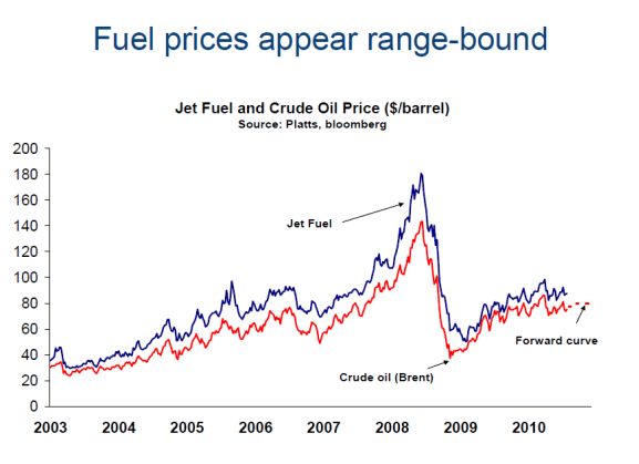
Real Options Valuation in the Airline Industry

                                         BMI Paper
                                   Author: Chuck Yuen Liu
                       Program: Business Mathematics & Informatics
                  Supervisor KLM Royal Dutch Airlines: Marjolein van Reisen
                           Supervisor VU University: Sandjai Bhulai

 VU University Amsterdam                                         KLM Royal Dutch Airlines
 Faculty of Exact Sciences                                    Department Fleet Development
   De Boelelaan 1081a                                              Amsterdamseweg 55
   1081 HV Amsterdam                                               1182 GP Amstelveen
     The Netherlands                                                 The Netherlands
Preface
This BMI paper is one of the last steps towards the Master of Science degree in Business Mathematics &
Informatics at the VU University Amsterdam. The purpose of this paper is to analyze and solve a problem on the
crossing of Business, Mathematics & Computer Science.

The goal of this paper is to provide an advanced methodology in airline fleet planning for the decision of buying or
leasing aircraft. Research was conducted at KLM for the department Fleet Development & Aircraft Trading and
was done in light of replacing 5 Fokker 100s with 5 Embraer 190s. Although methodology is designed for this
event, the results are generally applicable for financing decisions and not limited to a specific industry.

I would like to thank Sandjai Bhulai despite his busy schedule for making the necessary time for supervising this
paper from the VU University Amsterdam and Marjolein van Reisen for giving me the opportunity to do such an
interesting project and providing the necessary support from the Fleet Development & Aircraft Trading
department.

Chuck Yuen Liu, April 2011
Executive summary
We will show how to decide between leasing and buying aircraft using real options analysis. The theoretical
grounded methodology takes into account different scenarios and different options in a correct and fair way.

The choice for a firm above a lease is a matter of commitment, the more commitment is chosen the less flexibility
(implicit and explicit options) is available to management. At the other hand in normal market circumstances,
more flexibility costs more on the long term. We provide a general framework in which the financing decision is
made transparent and a new decision rule is introduced to make the tradeoff between profitability and flexibility.
The financing decision will eventually incorporate all possible scenarios of the future concerning the factors that
determine the profit or loss.

Main Goals:
   -   Provide a sound and objective guide to the financing decision
   -   Decompose the financing decision
   -   Provide a framework to do the necessary calculations
   -   Show how options can be valued
   -   Determining the optimal financing mix

Furthermore the methodology is implemented in an Excel valuation tool in which calculations are automated.
Additionally a manual gives insight in the usage of the tool and validation Excel sheets provide the validation of the
calculations mimicking in a step by step approach mimicking the final valuations.
Contents
1     Introduction ...........................................................................................................................................................7
    1.1        Background ..................................................................................................................................................7
    1.2        Problem statement ......................................................................................................................................9
    1.3        Structure of report .....................................................................................................................................10
2     Translate financing mix to real options framework .............................................................................................11
    2.1        Choices & Assumptions ..............................................................................................................................11
    2.2        Investment horizon ....................................................................................................................................11
    2.3        Comparing financing constructions ...........................................................................................................11
      2.3.1        Characterizing different financing constructions ...................................................................................13
    2.4        Overview of the decompositions of any construction ...............................................................................14
    2.5        Real options framework .............................................................................................................................16
      2.5.1        Expanded NPV........................................................................................................................................16
3     Investment analysis .............................................................................................................................................18
    3.1        Investment valuation .................................................................................................................................19
    3.2        Revenues ....................................................................................................................................................19
      3.2.1        Modeling the relationship between RPK, GDP and Yield.......................................................................20
    3.3        Costs ...........................................................................................................................................................21
    3.4        The risk factors ...........................................................................................................................................22
      3.4.1        Determining the investment and option value ......................................................................................23
4     Option valuation in discrete time ........................................................................................................................24
    4.1        Assumptions in the binominal tree model .................................................................................................24
    4.2        One period binominal tree model ..............................................................................................................24
    4.3        One period binomial tree model option valuation ....................................................................................24
      4.3.1        Revised Expectation: change of measure                                      .................................................................................26
      4.3.2        No arbitrage ...........................................................................................................................................27
      4.3.3        An example ............................................................................................................................................27
    4.4        Option valuation over two periods ............................................................................................................29
    4.5        Option valuation over n periods ................................................................................................................30
    4.6        Binomial representation theorem .............................................................................................................31
5     Option valuation in continuous time ...................................................................................................................32
    5.1        Probability space ........................................................................................................................................32
    5.2        Stochastic processes ..................................................................................................................................32
      5.2.1        Brownian motion ...................................................................................................................................32
      5.2.2        Variation ................................................................................................................................................33
      5.2.3        Stochastic integrals ................................................................................................................................34
      5.2.4        Itō’s Lemma ...........................................................................................................................................34
5.3 Geometric Brownian motion......................................................................................................................35
5.4 Understanding Geometric Brownian motion .............................................................................................35
5.5 Ornstein–Uhlenbeck process (Mean reversion) ........................................................................................36
5.6 Doob martingale ........................................................................................................................................37
5.7 Girsanov theorem ......................................................................................................................................37
5.8 Brownian Martingale Representation Theorem ........................................................................................38
5.9 Discounted investment under Q ................................................................................................................38
5.10 Valuing the option in the general univariate case .....................................................................................38
6 Multivariate option valuation in continuous time ...............................................................................................39
6.1 General n-factor model ..............................................................................................................................39
6.2 Theorems in multivariate setting ...............................................................................................................39
6.3 Valuing the option in the general multivariate case ..................................................................................39
7 Applying real option valuation ............................................................................................................................41
7.1 Three different options ..............................................................................................................................41
7.2 Justification of option valuation using simulation .....................................................................................41
7.3 Implementation in Excel ............................................................................................................................42
7.4 Determining the parameters of the stochastic factors ..............................................................................43
7.5 Calculation steps ........................................................................................................................................43
8 Conclusion ...........................................................................................................................................................44
9 Further research ..................................................................................................................................................451 Introduction
1.1 Background
The department Fleet Development & Aircraft trading is responsible for the procurement, financing and the sale of
aircraft within KLM. Procurement of (new) aircraft is an investment decision, a decision that has been made by
management in the light of bringing positive return to the company. This means a profitable investment in terms
of euros and/or a better strategic position. When aircraft needs to be replaced due to aging, the situation is the
same and the following question arises: How many aircraft is KLM going to invest/replace? KLM could choose for a
smaller number (reducing the fleet size), an equal number (keeping the same fleet size) or even a larger number of
aircraft (expansion of fleet). The next step in the process is choosing the financing construction, that is the choice
between buying (firm) and leasing. In this paper the focus is on unravelling and making the financing decision.
The choice of buying or leasing depends on the advantages and disadvantages accompanying a firm or a lease. For
each, one can distinguish two financing constructions. Buying gives us the choice of going for a financial lease or no
financing, i.e. paying the aircraft in steps to a bank willing to finance or paying the full amount before delivery to
the original equipment manufacturer (OEM) respectively. No financing has a big impact on the liquidities’ position
(and gearing ratio), as the entire sum is paid before delivery (pre delivery payments) and at delivery. Buying results
in ownership over the aircraft, in contrary with leasing where the aircraft returns to the lessor at the end of the
leaseterm. In the latter case the risk or uncertainty of the residual value of the aircraft lies with the lessor.
Leasing consists of two choices that are similar. KLM could directly go to the lessor and lease an aircraft which is
called an operational or direct lease. The other way is first purchasing an aircraft, immediately selling it back to a
lessor with the agreement for a direct lease. This is called a sale and leaseback construction. The advantage is that
KLM can customize the aircraft from the OEM, while in the direct lease there might be some restrictions as one is
dependent on the fleet of the lessor. Next to that it could be attractive to lease a relative short period when KLM
expects in the near future developments will change our choice, for example when a new fuel efficient aircraft
type is going to enter the market.
Financial lease
vs.
No financing
Buy
Invest in
vs.
aircraft
lease
Direct lease
vs.
Options Sale and
leaseback
Investment decision Financing decision
1.1 red – investment decision, green – delaying investment – blue – financing decision
In reality the financing decision is even more complicated. When one chooses to firm, one can acquire option(s)
from the OEM to purchase additional aircraft. The decision to invest can then be delayed at some moment in the
future, typically 1-2 years later. In 1-2 years time, one can decide to exercise the option and acquire the extra
aircraft for a predetermined price. This purchase option is valuable, if the investment decision can be made better
in 1-2 years of time.Options are not solely available in firms, in the direct lease (and sale & lease back) agreement we could obtain an
option to extend the direct lease with for example 2 years for a predetermined rate today. We will call such an
embedded (explicitly stated) option, an extension option.
As u might have noticed investing in options is neither an investment nor a financing decision, as the decision to
invest (and consequently the financing decision) in an aircraft is not made yet. But an option is valuable as it gives
us opportunities and no obligations, we must value these options just as any investment for full picture. The choice
to invest in options (as options typically costs money) is an investment decision in the option but not in an aircraft
(yet).
We have now made an overview of 5 ways to fill in our financing decision. We give an overview of the available
constructions we will take into account in this paper:
• Lifetime typically 20 years (new aircraft)
No Financing • Entire payment at beginning
• Risk: residual value
• Duration: typically for 10-20 years
• Fixed monthly fee
Financial Lease • Risk: residual value
• Cancellation Fee negotionable, prepayment option
• Duration: typically for 6-12 years
Direct Lease • Fixed monthly fee
• Can contain extension option
• Idem Direct Lease, but with involvement KLM
Sale & Lease Back purchasing the aircraft. Additionally purchase option
can be obtained from OEM.
• Duration: typically for 12-24 months
Purchase option • Predetermined price for develivery at some pretermined
date in the future. Typically for 20-24 months after
expiration option.
1.2 7 Financing constructions
The available financing constructions and the accompanying conditions like lease prices and durations are all
dependent on today’s market consisting of the Original Equipment Manufacturers (e.g. Boeing, Airbus, Embraer) &
the lessors and the negotiations between KLM and these market participants.
The eventual choice will depend on the uncertainty of the return on an investment and the price of a contract with
one of the market participants. The more uncertainty there is, the more flexibility is needed for management to
act accordingly in the then prevailing economy in the future. The flexibility lies in the duration of the financing
construction and options, a shorter lease term and/or options will give more flexibility in readjusting the fleet size
over time.
When for example choosing a 6 year direct lease over a 12 year direct lease, we get more flexibility as we can
reconsider the investment after 6 years. In other words we only committed to direct lease payments for 6 years
instead of an investment of 12 years which includes 12 years of costs. Choosing for 6 years however, will likely
result in a higher monthly payment. This will lower downside risk or losses in a bad state of economy but will limit
upside potential in a good state of economy.
The last important difference between the buying and leasing is the residual value risk that comes with buying.
Predicting the residual value in 20 years time is hard as many factors have to be taken into account.Clearly, there are pros and cons for each financing choice and it is the goal of this paper to evaluate the pros
against the cons in an objective way. In this paper we take on a mathematical approach using real options
valuation to solve this problem.
1.2 Problem statement
Now that we have a full picture of the available constructions, we are ready to formulate the problem statement.
The situation is as follows: The investment decision is made for x airplanes and we are up to the challenge how to
allocate the number of aircraft to the five different constructions, where each construction takes up one
allocation.
Example
KLM has decided on the investment of 5 Embraer 190’s, to replace 5 old Fokker 100’s in operation. The question is
how to allocate the 5 “slots” over the available constructions.
– One possible allocation or mix of financing is:
all 5 Direct Lease for 10 years (without extension options).
– Another possible allocation is:
1x Direct lease for 8 years (without extension options),
3x financial lease for 20 years and 1 purchase option maturing in 1 year for delivery in 2 years time from
option maturity.
– Another possible allocation is:
3x Sale and lease back for 8 years $0.25 million per month with each an extension option to extend by 2
years and 2x a purchase option.
KLM has these three financing mixes available and has to make a decision which one to choose. The choice will
depend on the price, the flexibility a mix provides, upside potential and downside risk for the final choice.
Financing choices
Tradeoff to be made A financing mix
Financial
Lease Price
No
Direct
Purchase Purchase lease
Financing options
options
Upside Financial
potential lease
Direct Lease Sale and &
Lease Back Downside risk
1.3 Find the ideal financing mix, identify the available constructions, measure their pros and cons and make the choice.We formulate this in a formal research question.
Research question
• What is the optimal mix of financing for the acquisition of a fixed number of new aircraft given its current fleet
and today’s financing market?
With the following sub questions:
◦ How to reformulate the financing decision into the real option valuation framework?
◦ How do we define optimal?
◦How to value options?
The valuation of the different financing construction is not possible with the well known Net Present Value (NPV)
or Discounted Cash Flow (DCF) method. The reason is that options are differently valued than investments and the
NPVs of different lengths of contracts cannot be fairly compared to each other. We can translate the financing
question into an option framework and use financial options theory to value the options properly, in the next
chapter one will also see that it resolves the unequal “investment horizons”. The valuation of the options in the
option framework will lead us to the optimal financing mix.
1.3 Structure of report
The structure of this paper is as follows:
Choice of optimal financing mix
Translate financing mix to real option framework
Investment analysis Option analysis
Translating the financing mix to the real option framework is treated in chapter 2, in chapter 3 investment analysis
is treated and the mathematical approach to option analysis is treated in chapter 4, 5 & 6. In chapter 7 we come to
the application of the theory to come to the optimal financing mix using an alternative (insightful) way of option
valuation. The alternative approach is implemented in Excel. We finish with our conclusion in chapter 8 and in
chapter 9 a word on further research directions.2 Translate financing mix to real options
framework
In this chapter we will answer the first sub question:
- How to reformulate the financing decision into the real option valuation framework?
2.1 Choices & Assumptions
- Although it is possible to do a sale and leaseback for any aircraft in ownership, we will assume here that
this can only be done at the moment of the financing decision, today.
- Escalation of lease payments is assumed to be fixed, thus non-stochastic.
- The analysis assumes aircraft are delivered straight away at initiation of the contract.
- Options are decided on at maturity and delivery of the optional aircraft is instantaneous too.
- When ownership is chosen, we assume the aircraft will be operated on for its natural lifetime typically 20
years after which the aircraft is sold against market value.
2.2 Investment horizon
To compare financing mixes in a fair way, we need to compare financing constructions over an equal time interval.
It matters whether we invest for 8 years or for 20 years and a fair comparison is needed. There is a 12 years
difference between the two, after the 8 years investment one can make the decision to reinvest or not. These 12
years are an (implicit) optional investment, and by seeing it as an option one can value it accordingly. Thus the
total period to consider is 20 years called the investment horizon. If we have an 8 year direct lease contract and
there are 2 extension options available for 2 extra years, the investment horizon of this contract is 8+2+2 = 12
years. Comparing it with a 20 year investment, we would value the remaining 8 years of the direct lease as an
option again.
We will formally define the above:
Definition: Investment horizon of a financing construction
The Investment horizon of a financing choice is the operation time plus, if present, the extension time for optional
operation (due to options).
The next step would be to compare financing mixes, we take the maximum of the investment horizon of all the
available financing constructions and consider that the investment horizon for fair comparison.
2.3 Comparing financing constructions
The real options framework is simple. By looking at the investment horizon for all the contracts we can fairly
compare them. By definition one financing construction has the length of the investment horizon of the financing
mixes. The other contracts are equally compared by realizing we have an opportunity, an implicit option, to
reinvest at the end of a contract. This implicit option is a reinvestment option.A financing construction
Attractive
forecast
revenues
Start
Investment
horizon: End of End
Initiation delivery aircraft investment
contract aircraft usage horizon
Investment Optional investment
Investment horizon
Example 1:
Consider the situation where we want to compare two direct lease contracts with lengths of 6 and 12 years in the
contract.
If we would have invested in the 6 years contract, we have an option after 6 years to do a reinvestment for the
remaining 6 years. In practice this is a bit before the 6 years, as the contract negotiation and delivery time needs to
be taken into account but for convenience we assume this is exactly after 6 years. We can either decide to replace
the aircraft or decide not to reinvest. This will depend on the economic outlook and the cost of ownership for a
replacement airplane. In case the aircraft is forecasted in year 6 to be loss making then the reinvestment option
will not be exercised and the fleet size will decreases by one. At the other hand when market circumstances
present themselves favorable we can use our option and reinvest in the remaining 6 years.
If we have chosen the 12 year direct lease, there wouldn’t be flexibility after running 6 years in the contract. We
would be obliged to continue operating the aircraft and satisfy the lease payment in both favorable and
unfavorable market circumstances.
Example 2:
Consider the situation where we want to compare a direct lease contracts with a length of 12 years against a
financial lease with a duration of 16 years.The duration of the financial lease only states the period to pay and the aircraft at the end of the contract is still in
ownership of the airliner. Thus the length of the financial lease contract is irrelevant. Assuming the aircraft has a
lifetime of 20 years, the investment horizon to consider is 20 years. If we would choose for the 12 year direct lease
we would have a reinvestment option at year 12 for a period of 8 years. This is flexibility which the financial lease
contract doesn’t offer.
2.3.1 Characterizing different financing constructions
All the financing constructions can be decomposed in an investment (indicated blue) and option component
(indicated green). The investment component consists of the price or lease rate to be paid, a duration the aircraft
can be operated and whether ownership is obtained or not. The duration available for operation is in the case of a
direct lease or sale and lease back, the duration of the contract and in case of a firm (i.e. “No financing” or
“Financial lease”) the natural lifetime of the aircraft (typically 20 years) before KLM would sell the aircraft. The
ownership of an aircraft is obtained only in case of a firm. In case of ownership, one receives the sale proceeds of
the aircraft at the end of its natural lifetime.
Options can be an extension option in case of a direct lease, a purchase option in case of firm or a reinvestment
option in case the operation duration of a specific contract is shorter than the investment horizon. The investment
can be valued with the traditional NPV method, while options need to be valued appropriately using discussed in
later chapters.
Any financing choice
Investment Options
Price Duration Ownership Contract Reinvestment
of operation option option2.4 Overview of the decompositions of any construction In this section we give a complete overview of all financing constructions. We will visualize the cash flows accompanying each financing construction. That is the payments for the right to use an aircraft (e.g. lease payments) and the sale proceeds when dealing with a firm. Additionally the direct lease and sale and leaseback are similar in our analysis, we assume that the sale and lease back terms from the OEM and lessor to can be determined and is executed today. So that we don’t take into account the opportunity to firm and sale and lease back and aircraft in a later stadium. That is a firm stays a firm. As a consequence the difference between a direct lease and sale and lease back lies in the availability of purchase option(s) for the latter one.
Sale and
No financing       Financial lease       Direct lease
                                                               Leaseback

                                                               NPV investment
 NPV investment      NPV investment      NPV investment
                                                               during duration
 during lifetime     during lifetime     during duration
                                                                  contract
     aircraft            aircraft           contract

                                                               Extension option
 Residual value      Residual value     Extension option

                                                             Reinvestment option

 Purchase option     Purchase option   Reinvestment option
                                                               Purchase option
Finally we conclude this paragraph with the visualization of an option. As can be seen we have assumed that whenever the option is exercised at maturity, the optional aircraft is delivered immediately. 2.5 Real options framework Having gone through the previous sections, we have all the tools to reformulate the allocation or financing question into the real options framework. If the duration of the available contracts were the same and no options were present, then the Discounted Cash Flow method (DCF) or the Net Present Value (NPV) method is the right choice. In the previous section we saw the difference in time as a reinvestment option. Valuing all other options we can fairly compare and value financing constructions. We can integrate the value of the option with the NPV to come to the financing decision. The fixed component is here the initial commitment to the investment, so in a direct lease this is the duration of the contract while the variable component consists of all the options that come available given that one has chosen for a specific contract. With the explicit options being the purchase and extension options and the implicit options being the reinvestment options. 2.5.1 Expanded NPV The integration of both the NPV of the project during the contract time with its options leads us to the expanded NPV. The static part or fixed part of a financing construction valued with the NPV method is called the static NPV, this name follows from the fact it fails to incorporate the flexibility in options and only values the fixed component of a contract. The value of the implicit and explicit options in the financing construction is the option premia. Adding the values up, we get the Expanded NPV. Definition Expanded NPV Expanded NPV = Static NPV + Option Premiums The expanded NPV was introduced by Gehr in 1981 and is used by Trigeorgis (2001).
We would calculate the expanded NPV for each financing mix, and just like a normal NPV analysis we choose the
project that has the highest NPV, but now the expanded NPV which also incorporates options.

An example:
If today the investment decision is made for 5 aircraft, two different financing mixes could be:
     -    2 direct Lease for 12 years, 2 financial lease for 20 years and 1 purchase option (maturity in 1 year).
     -    4 direct lease for 10 years and 1 financial lease for 20 years.
Translating this into the real options framework:
     -    Mix 1: 2 direct lease + 2 options starting in year 12 to reinvest for 8 years + 2 financial lease + 1 purchase
          option.
     -    Mix 2: 4 direct lease for 10 years + 4 options starting in year 10 to reinvest for 10 years direct lease + one
          financial lease for 20 years.

This would yield the following expanded NPV:

Expanded NPV mix 1: 2x NPV direct lease for 12 years + 2x Option value direct lease in 12 years time + 2x NPV
financial lease for 20 years + 1x purchase option value
Expanded NPV mix 2: 4x NPV direct lease for 10 years + 4x Option value direct lease in 10 years time + 1x NPV
financial lease for 20 years. The obvious decision is choosing the financing mix which holds the highest expanded
NPV and can be seen as the expected added value given one chooses for the corresponding financing mix. This is
also the answer to the second sub question, how optimality is defined. The choice here is made on the highest
expected return, the highest expanded NPV among all possible financing mixes.

In general it holds that the higher the uncertainty, the higher the options are in value. The choice will depend on
the amount of uncertainty. The lower the uncertainty the more the expanded NPV will move towards firm (that is
going for ownership: No financing or Financial lease), since the options will be worth less. The higher the
uncertainty the more the expanded NPV will tend towards flexibility, the options will become more valuable (as
having the choice to invest is available) so that shorter contract durations (gives reinvestment options) and
purchase options and extension options are preferred.
3 Investment analysis
In this chapter we will view investments from a financial theoretic point of view.
In investment analysis one always has to make the tradeoff between risk and return. In general the more risk one
is willing to take, the higher the promised or expected payoff is. Investors get compensated for risk. The starting
point of any investment analysis in financial literature is identifying a so called risk free rate, which is the rate of
return of an investment without any risk. One could say that putting money into a savings account is safe and risk
free. In general banks are reliable and even when a bank defaults, most governments still guarantees the savings.
The interest one receives can thus be considered to be the risk free rate. For corporate investments, sovereign
bonds are considered risk free and more specifically triple A bonds like German (or Dutch) bonds. We will make the
assumption that the risk free rate exists and equals the rates of German bonds. One could still debate between
bonds of different lengths, we follow market conventions by taking 1 year bonds.
As a consequence the rate of return of any investment project that has no risk, is the risk free rate. Any risk free
cash flows in the future should be discounted by the risk free rate to get the fair value of the investment today.
In the corporate world cash flows of investment projects are far from certain. This has given the rise of different
risk adjusted discount factors or risk adjusted rates of return like the weighted average cost of capital (WACC)
within corporations. Observe this is always higher than the risk free rate, this rate of return can be seen the
required expected rate of return for an investment within the corporation.
The WACC depends on the industry and also varies across firms, as different industries have different degrees of
risk and different firms have different risk appetites. One can imagine that the risk of a budget airliner/low-cost
carrier is different than from a legacy carrier (which targets different customers). Within KLM two WACCs or
discount rates are used for investments in aircraft, 4,5% for the replacement of fleet and 9% for the expansion of
fleet. The higher required rate of return for expansion of fleet underwrites the higher risk and thus results in more
uncertain cash flows when one expands the fleet.
In the next chapter we will show how we are going to deal with the risk of the option or the uncertainty of the cash
flows associated with the option. One has to distinguish between the risk or uncertainty of today (the initiation of
the option) till the maturity of the option and from this maturity till the end of the (optional) investment. On
maturity of the option, we cannot postpone the decision anymore whether to invest or not. Using the risk adjusted
WACC one can calculate the added value of the investment at that moment. One can view the calculated added
value as the payoff of the option at maturity whenever it is positive. When this amount is negative, the optional
aircraft is not exercised. No value is added but also no costs are incurred. The question remains what to do with
the uncertain payoff between today and the maturity of the option. It would be incorrect to use the risk free rate
as the payoff is uncertain. Essentially there are two ways to resolve this:
1) Use a risk adjusted discount rate, e.g. the WACC at 4,5%. State the risk of the optional aircraft investment
equals the risk on the replacement of an aircraft.
2) Use financial option valuation.
In the later chapters we explain the mechanics of financial option valuation. We will prove that the payoff of an
option can be replicated with an hedging portfolio. The consequence is that all risk is hedged away. As a result we
can value the option by discounting the value of the replicated portfolio at maturity (which is the payoff of the
option at maturity or the payoff of the investment at maturity), with the risk free rate. In general the risk free rate
is the only discount rate that is used in valuing options using the replication argument.
Although we explain financial options valuation, for the implementation we will choose the other option. That is
pricing the risk with another risk adjusted discount rate like the WACC. Financial options theory is highly
complicated and hard to fully understand by first encounter, while the WACC methodology can be explained moretransparent. Nonetheless, we will be needing a part of the theory of financial options valuation to do the first
option.
Below we show we plot of the value of the option over time, once can observe that this changes over time and
secondly the volatility decreases the closer to the end. That is when the option option is exercised at the maturity
of the option, the revenues and costs will be more and more set. The plot also show there is two different risks or
uncertainties having an option. The first risk is the start time of the option till maturity, which is the uncertainty of
the value of the option while having the opportunity to exercise or not. And second is the risk or uncertainty once
the option is exercised, which is the risk of the investment itself.
Development of the profitability of the optional ac
Initiation
Option
Eventual
payoff
Maturity investment
option
Risk of option Risk of the investment
Time in years
Today 2 4 6 8 10 12 14 16 18 20 22
3.1 Investment valuation
At the time the decision about the investment has to be decided upon, the project to be invested in needs to be
valued. One needs to make an analysis of the expected cash flows, that is the revenues minus the costs for the
duration of the investment and discount it back using the appropriate risk adjusted discount factor WACC. This is
normally done on a yearly basis and in this paper the analysis will also be. The revenues and costs will be zoomed
in and is the basis for the valuation of the investment and the option. Note that in case of a firm, the residual value
of the aircraft at the end of its natural lifetime needs to be taken into account in addition to the revenues and
costs and is a risk factor as well since there is uncertainty about the residual value of an aircraft at the end of its
lifetime.
3.2 Revenues
The income stream of an aircraft is determined by the revenues from ticket sales. In the aviation industry one
denotes the revenues in the realized revenue per passenger per kilometre (RPK) and in yield per RPK. In this
context RPK is not an amount from revenue but the actual realized occupied seats that travel a kilometre. Yield
means the actual revenue or money units that the passenger has paid (by average, think about business andeconomy class) for this one seat per kilometre. From this it follows that the revenues are given by the following
equation (all variables are per year):
Once the investment must be decided on, the then prevailing yield and RPK in that specific year is assumed to be
known.
The yield will depend on the type of aircraft and the specific area of operation of the type of aircraft. For example,
the Embraer 190 has a yield that is for 1/3 dependent on the yield of intercontinental flights and 2/3 dependent on
the yield of regional flights. Thus the yield for this type of aircraft can be computed to be the weighted average of
the intercontinental and the regional flights. The two yields from the regional flights and intercontinental flights
are the weighted average of the yields from the economy classes and business classes.
Furthermore we assume a constant network utilisation, that is the planned number of kilometres and number of
flights each year for the total fleet of this type remains constant. Also all planned flights (and their corresponding
kilometres) are assumed to be carried out. So that in the valuation we assume that aircraft keep flying even for
example when the yield fall.
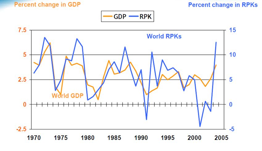
3.2.1 Modeling the relationship between RPK, GDP and Yield
We acknowledge the fact that the RPK generated by the fleet is dependent on the world gross domestic product
(GDP). When GDP goes up, the RPK (Revenue per passenger kilometre) generated by KLM’s fleet goes up too.
3.1 Source Boeing 2008
Next to GDP, RPK is dependent on the yield. Whenever yield goes up (tickets prices rise) demand expressed in RPK
will go down. We model this (deterministic) relationship in the following equation.
Where the elasticity’s are assumed constant.
The relationship tells us that when GDP goes up with 1%, the RPK will go up by approximately %. And when yield
goes up with 1%, the RPK will go down with approximately %. Approximately, since the changes are log
proportional. Given a yearly change of the GDP and yield and the corresponding elasticities and , we candetermine the RPKs. From this it follows that the revenues can be determined by GDP and yield, which are
unknown for the future from today’s point of view. Thus these are stochastic.
3.3 Costs
Likewise with the revenues, we take the total costs per year and assume constant network utilization and following
that a constant fuel consumption.
Where the costs are divided in:
E&M = engineering and maintenance.
Flight operations = operational costs including take off and landing charges by Schiphol and other airports.
Ground & Handling = costs incurred with baggage handling
Catering = costs occurred with meals by passengers and crew.
Other (Sales, Costs
Commission,)
7%
Ownership's
11% E&M
16%
Fuel Crew
15% 18%
Flight Ops
Ground&
12% Catering
Handling
4% 17%
3.2 costs pie based on 07/08 Fokker 100, E&M heavily dependent on age of ac
From an investment point of view, the fuel costs are the biggest risk factor. We assume that E&M, Crew, Ground &
Handling, Catering & Flight Operations are deterministic costs and in jet fuel lays the uncertainty when considering
the costs of the investment over the investment horizon. Thus jet fuel becomes a stochastic factor to consider. The
jet fuel price is primarily influenced by the crude oil price quoted in financial markets. The costs excluding fuel and
ownship will be put under either fixed or variable costs of which the total variable costs are divided equally over all
the aircraft. We could think of the fixed costs as costs due to ground staff which does in essence not depend on the
fleet size (under small mutations) while the variable costs like catering is dependent on the fleet size.3.3 Source IATA
We will assume that the correlation between jet fuel and crude oil prices is perfect and work with a (constant
assumed) conversion factor to jump from jet fuel consumption to crude oil consumption.
For the ownership costs we need to distinguish between the ownership costs if we would make the investment
today and in the future. Today the ownership costs are known. These stems from the lease conditions and the
buying terms which are the results of negotiations between KLM and the corresponding lessors, financing banks &
OEMs. In contrary the ownership costs in the future are uncertain, the profit from an (implicit) option to reinvest
depends on the ownership costs by that time. While the ownership costs for purchase options and extension
options are part of today’s contract.
For today’s investment we would need to give an estimate of all three components for the time of the investment.
The biggest uncertainty lies with the fuel and a prediction of the fuel costs in the future needs to be made. This
depends on the beliefs of experts and/or in combination with a model to predict crude oil prices. Since from the
costs perspective, oil and ownership costs are the biggest risk factors we model these two as risk factors while
taking the variable and fixed costs deterministic (constant per plane). The ownership costs in the future are
stochastic too and we will simulate a direct lease rate (where we don’t distinguish between lease rates of different
lengths) to get a proxy for the ownership costs in the future.
3.4 The risk factors
We have determined that the risk for the investment in aircraft are determined by 5 different risk factors which
are risks because the development of these factors determine the attractiveness and unattractiveness and are
uncertainty (stochastic). Tthey are unknown from the perspective of today. Quantification of risk is done by
dispersion and the volatility is one common to quantify risk. The later chapters on option valuation will make use
of the volatility and see this a parameter in the stochastic model.
Fuel Residual Lease
GDP Yield
price value rate
3.4 The volatility of the option is the volatility of all these (correlated) factorsThese factors change all the time and the investment decision is primarily based on these factors i.e. the projected
revenues and the forecasted costs.
3.4.1 Determining the investment and option value
We look at the investment from a financial perspective, the value of the investment is determined by discounting
future cash flows with an appropriate discount rate. The future cash flows are determined by the 5 risk factors and
are unknown/stochastic at the moment the investment has to be decided on. At that moment one has to forecast
the 5 factors for the investment horizon to determine the cash flows. In this paper we will assume that the 5
stochastic factors follow some stochastic process, elaborated in the option valuation chapters. This can capture
both stable future levels for the factors as well as disperse changing behaviors.
Implementation wise, this means we will simulate the factors for different scenarios and from that determine the
profit = future revenues – future costs, this is a generalization of Paul Clark’s approach on fleet planning using the
macro approach to investment valuation (2007). In which the revenues of an additional aircraft are determined by
first allocating the RPKs (=market demand) to the “fixed” fleet (the fleet from contracts which is not optional). The
new aircraft takes the “leftovers” in terms of RPKs. Capacity in terms of passenger kilometres is denominated by
available seat kilometres. From a revenue management perspective it is known that aircraft cannot be filled up
100%, the ASKs (=available seat kilometres, the maximum capacity of an aircraft) without influencing the yield
level significantly. That is why we assume there exists a maximum load factor, which we will use to determine the
maximum RPK one aircraft can generate.
The value of an option goes in the same fashion, since at maturity of the option the situation is the same: a
projection of revenues and costs has to be made on the basis of the current levels of the 5 factors. The following
steps are undertaken:
The projected revenues = projected yield * projected RPK.
At maturity of the option, the decision moment, we exercise the option if:
1) Demand RPK cannot be covered by ASK without optional ac
Projected RPK > ASK without optional ac * maximum load factor
and
2) “Spill” RPK is profitable:
projected yield*(Projected RPK-ASK without optional ac * maximum load factor) > projected cost optional ac
Else the optional aircraft is not profitable. We do nothing and let option expire to invest.
*Projected RPK (which is the total RPK generated by the entire fleet) is also dependent on the current fleet, as the
current fixed fleet size changes during this evaluation period. We assume the fleet size, which are not in the
financing decision today, stays constant over the investment horizon.4 Option valuation in discrete time
Option valuation in discrete time means that time is partitioned over a countable number of intervals at which the
option is valued. We will start off with option valuation over one period and then generalize to multi period
analysis. These are important examples as these are fundamental towards continuous time models which we will
eventually use.
In general one needs to define the behavior of the value of an investment or project, this behavior is a process
which is uncertain from today’s point of view and thus stochastic. The value of the project will be called S and its
value at time t is . All options that we consider are call options.
4.1 Assumptions in the binominal tree model
a. There exists a risk free bond discount bond with continuously compounded interest rate
b. One can borrow money at the risk free rate
4.2 One period binominal tree model
The binominal tree model specifies the process of the value of the project S, assuming that the process either goes
up or goes down. The constants are assumed to be known and satisfy d < u and 0 < p < 1:
“The starting value at time 0 of the process is known and is ”
“At time 1 the process increases in value with factor u with probability p”
“At time 1 the process decreases in value with factor d with probability p”
The choice of this discrete time model can be motivated, as this process converges to the continuous time
Geometric Brownian Motion model which we will consider later on.
4.3 One period binomial tree model option valuation
The one period binominal tree model can be visualized as follows:
The evolution of the investment
Time 0 Time 1
Where the value of the process at time 0 is known and the value of the process at time 1, is unknown.
takes on the value or with probability p and 1-p respectively. In same fashion the
option value at time 0 is known and the option value at time 1, is unknown. takes on the
value and . The functional form or claim of a call option at maturity T is
. We can derive the value of the option where K is a constant. In other words the option becomes valuable
when the project value exceeds the threshold K and the option is consequently exercised. Else it is not exercised.
Thus for an option to make sense in the one period model, it must hold .The evolution of the option’s value
Time 0 Time 1
The question now, what the fair value at time 0 of an option that expires is at time 1 when the investment decision
needs to be made today. As one can notice the value of the option is uncertain and holding it results in risk or
uncertainty about the eventual option value at time 1. It turns out that we can compose a portfolio at time 0 and
without risk this portfolio will always replicate the option value at time 1.
Construct a portfolio at time 0, . Invest a fraction in the investment and invest a fraction in a risk free
bond that matures at time 1. In mathematical notation: The portfolio at time 1 equals
The discount bond will increase in value to and the process turns into
which is or with probability p and 1-p respectively. Note we use the continuously compounded interest
rate for the bond price process, instead of a periodic compounded in which case . This choice does
not change the theory except some notation for discrete time models but will come in handy for continuous time
models.
Now we want the portfolio at time 1 to replicate the option value at all times, when the project
increases in value as well when the project decreases in value.
This results in the following two equations at time 1:
We point out that the only unknowns are the fractions , and hence with two equations and two unknowns we
can solve for , .
We get
and
= =
So for these two choices of and , our portfolio replicates the option’s payoff at time 1. Note that the
probability p of an upward movement is irrelevant!4.3.1 Revised Expectation: change of measure In the previous section we derived an explicit formula for ( ). Since the option value and the replicating portfolio at time 1 are equal (enforced by the two equations) we can find the option value at time 0 by filling in the portfolio weights ( ): The subscript in the expectation operator means we have to replace the real probability p with the new defined q to evaluate the expectation. Thus the option value can be evaluated as the discounted expectation under a new probability measure , defined above. The correct price of the option is not the discounted expectation under the real physical measure , that is the real probability of going up and down in value. Calculating the price of the option using this new measure is just an artificial way of changing the probabilities in such a way that the fair price of the option is found. If one would use the real probabilities one would be evaluating the value of the option through its expected payoff. Doing so one does not take into account the risk of the option. This is only valid when investors are indifferent to risk or that investors are risk neutral. Taking the expectation under the measure to calculate the fair price of the option seems like as if risk is not taken into account, this is the reason why this is called risk neutral valuation. In fact the original expectation under the real probability p is adjusted with q and exactly this operation takes into account risk. As a consequence the new artificial probabilities (which are only used for computation for the option price) are called risk neutral probabilities. The third name to these artificial probabilities or the measure is the martingale measure. One can see that: A martingale is a variable that doesn’t change in expectation, that is the variable does not tend to grow or decrease over time but has as expectation the current (known) value. In general, a process Z is a martingale if it satisfies the following (with the subscript in Z denoting the time index):
We have left out the subscript on the expectation operation which denotes measure to use, typically one would
say it is a martingale with respect to a certain measure if it is needed to explicit specify it. In this paper processes
are typically a martingale with respect to but not with respect to the measure .

The variable is unknown from the perspective of time 0, we have shown that its discounted value, the
expectation is (given is known). We can make the known information explicit by writing the conditional
expectation:                       . The measure     is such that the variable S becomes a martingale, hence the
name martingale measure.

4.3.2 No arbitrage
In the previous section we saw that the option and the replicating portfolio have the same cash flows and thus
they are essential the some security. Since they are identical there should not be a reason why they would be
priced different, this is in economics called the law of one price. At the moment there is an imbalance in pricing,
there will be a higher demand for the cheaper security. This higher demand will results in a rise in the price of the
cheaper security until the two prices coincides again.

The Financial market allows short selling of securities. Whenever there are two securities that are identical or have
the same cash flows and they differ in price, one can buy the cheaper one and short sell the expensive one. At the
maturity of the security, one has covered its obligations and has a neutral position. The difference in price results
in a risk free profit. This is called an arbitrage opportunity. In financial markets no arbitrage is assumed as these
opportunities will disappear quickly whenever they become available.

As a consequence the price of the replicating portfolio equals the option price.

4.3.3 An example
Now we turn to a numerical example, we assume:

This results in the following visualization of the project value.

                                                                           The evolution of the investment

      Time 0                                       Time 1

From this we can derive the call option on such a project:
The question is what the value is of the option at time 0, .
The evolution of the option’s value
Time 0 Time 1
We answer this by valuing the replicating portfolio:
The second weight is negative, it would mean we wouldn’t buy the bond but short sell the bond against the
interest free rate.
Now we construct our portfolio at time 0:
Now one period later we have:
We just exactly replicated the option buying 8/15 of the project and short selling 40 riskless discount bonds. As we
can see the payoff of the portfolio exactly replicates the portfolio of the option. Thus the option’s value is 15.238.
Alternatively we can derive the option value using the discounted expectation under the measure. This gives the
identical result as the portfolio value at time 0. We find the new probability measure and then evaluate the
discounted expectation under this artificial measure.
As one can see option valuation using an expectation under a new measure is quick, it is the way option pricing
is done in practice.You can also read