The Large Hadron Collider and the ATLAS Detector
←
→
Page content transcription
If your browser does not render page correctly, please read the page content below
Chapter 2
The Large Hadron Collider and the ATLAS
Detector

2.1 The Large Hadron Collider

The Large Hadron Collider (LHC) at CERN (the European Center for Nuclear
Research) is a 26.7 km long particle accelerator outside of Geneva, Switzerland [1].
It lies below-ground in the tunnel previously inhabited by the LEP machine. It is
capable of colliding particles at four different experimental sites, which are occupied
by the ATLAS, ALICE, CMS, and LHCb detectors.
    There are several principal parameters used to define the physics potential of a
particle accelerator:
                                        √
     • The center-of-mass energy, or s, is the total energy of a proton-proton system
        at an interaction point (in the lab frame).
    • A is the cross-sectional area of the beam at a collision point, and depends on the
      longitudinal and lateral spread of the proton bunches. It can be expressed as:

                                            4πεn β ∗
                                       A=                                         (2.1)
                                             γr F

      where εn is the normalized transverse beam emittance, β ∗ is the beta function
      (a measure of the beam width) at the collision point, γr is the Lorentz gamma
      factor, and F is a factor that accounts for the fact that the beams do not strike
      head-on, but rather cross with some angle.
    • The luminosity, L, is then defined as:

                                          fr ev n b N1 N2
                                    L=                                            (2.2)
                                                  A
      where fr ev is the revolution frequency of the beam, n b is the number of bunches
      in the beam, and Ni is the number of particles in each bunch. (Their typical
      values will be discussed in the following section.)

M. Hance, Photon Physics at the LHC, Springer Theses,                                17
DOI: 10.1007/978-3-642-33062-9_2, © Springer-Verlag Berlin Heidelberg 2013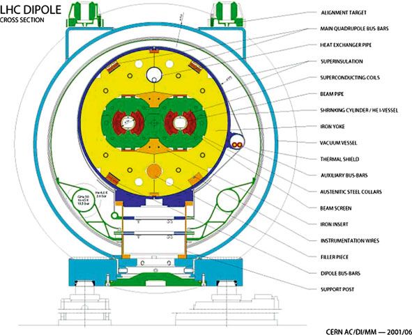
18                                       2 The Large Hadron Collider and the ATLAS Detector

Fig. 2.1 A cut-away view of an LHC dipole magnet. There sections of both LHC rings in each mag-
net, one for each beam. The rings are coupled magnetically, each having a flux of equal magnitude
and opposite sign to the other, and share mechanical and cryogenic services

   As a proton–proton collider, the LHC has a designed center-of-mass energy of
14 TeV and a designed luminosity of 1034 cm−2 s−1 . It is also capable of colliding
heavy ions (lead) at energies of 5.5 TeV per nucleon pair, with a peak luminosity of
1027 cm−2 s−1 .

2.1.1 Design

To achieve its ambitious goals for beam energy and luminosity, while meeting the
physical constraints of the LEP tunnel, the LHC was designed as a two-ring supercon-
ducting accelerator. The superconducting elements are Niobium–Titanium (NbTi)
coils, which are cooled to a temperature of 1.9 K through the use of 96 metric tons of
superfluid liquid Helium. The two rings share a cryogenic and mechanical structure,
and are coupled magnetically, each ring having a magnetic flux equal in magnitude
(but opposite in direction) to the other. A cut-away view of an LHC dipole is shown
in Fig. 2.1.
   Protons are accelerated in stages in the CERN accelerator complex, culminating in
their injection into the LHC at a beam energy of 450 GeV. The protons are injected in
bunches, with a maximum bunch size of roughly 1.5 × 10¹¹ protons (Ni ). There can
2.1 The Large Hadron Collider 19
in principle be as many as 3,564 bunches stored in each ring; in practice, not every
bunch is filled, and there is an effective maximum of 2,808 filled bunches (n b ). Each
bunch orbits the ring with a frequency of 11 kHz ( fr ev ). Bunch crossings occur at
each of the interaction points at a frequency of 40.08 MHz. At its design luminosity,
each bunch crossing will have roughly 20 proton–proton interactions.
After injection and acceleration, protons are circulated and collided for a long
period of time. This is known as a fill, and can last as long as 24 h. Over this time the
instantaneous luminosity will degrade as the protons collide and the proton bunches
slowly lose their integrity. A typical fill can see a factor of two (or more) drop in
instantaneous luminosity from beginning to end, depending on the length of the fill
and the stability of the beam.1
Even at the highest instantaneous luminosities, most bunch crossings will contain
only one hard (large Q 2 ) interaction. Additional proton–proton interactions in each
crossing are referred to as in-time pileup, and will typically contribute energy (in the
form of soft particles) homogenously throughout the detector. The effects of in-time
pileup on prompt-photon identification will be discussed further in Sect. 4.3. In addi-
tion to in-time pileup, the short bunch-spacing of the LHC beams means that the
detector response in a given bunch crossing can be influenced by the residual effects
of previous bunch crossings. Such out-of-time pileup effects will also be discussed
in Sect. 4.3.
2.1.2 Running Conditions in 2010
√
The LHC produced its first collisions at s = 7 TeV in the spring of 2010, and contin-
ued to run throughout the summer and fall at that energy. At first, there was a single
bunch per beam, with an average of less than one interaction per bunch crossing.
The beam conditions improved quickly over the summer and fall, and the instanta-
neous luminosity grew from 1027 cm−2 s−1 in April to over 2 × 1032 cm−2 s−1 in
November. At the end of the 2010 run, the LHC was averaging over three interactions
per crossing, with trains of filled bunches in each beam. The minimum bunch spacing
was 150 ns. A plot of the integrated luminosity delivered by the LHC versus time is
shown in Fig. 2.2.
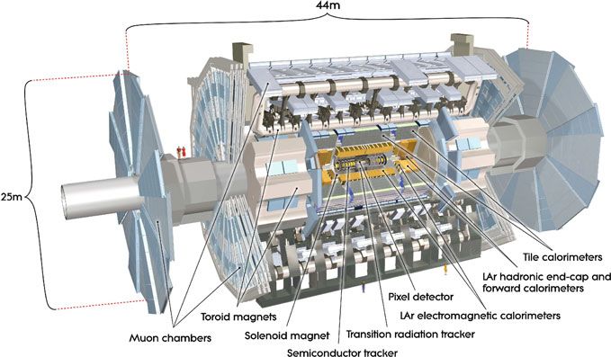
2.2 The ATLAS Detector
ATLAS (A Toroidal LHC ApparatuS) is one of two general-purpose detectors at
the LHC–the other is the Compact Muon Solenoid (CMS) detector. As with other
modern experiments, ATLAS was designed as a hermetic detector with the following
elements:
1 The luminosity lifetime (τ ) of the LHC beam is roughly 15 h; depending on the down-time between
fills, the optimal fill length is anywhere from 5 to 24 h [1].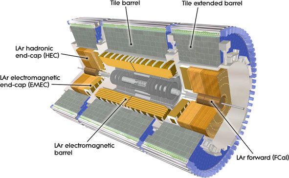
20                                                                                  2 The Large Hadron Collider and the ATLAS Detector

 Total Integrated Luminosity [pb-1]   60
                                           ATLAS Online Luminosity      s = 7 TeV
                                                                                                               4.5   ATLAS Online       s = 7 TeV

                                      50                                                                         4      LHC Delivered

                                                                                            Peak
                                               LHC Delivered
                                               ATLAS Recorded                                                  3.5
                                      40   Total Delivered: 48.1 pb-1                                            3
                                           Total Recorded: 45.0 pb-1                                           2.5
                                      30
                                                                                                                 2
                                      20                                                                       1.5
                                                                                                                 1
                                      10
                                                                                                               0.5
                                       0                                                                        0
                                       24/03     19/05         14/07      08/09     03/11                       24/03     19/05          14/07      08/09   03/11
                                                          Day in 2010                                                               Day in 2010
                                                               (a)                                                                        (b)
Fig. 2.2 The integrated luminosity (a) and the peak average interactions per crossing (b) delivered
by the LHC in the 2010 run

                                      • An inner tracking detector immersed in a solenoidal magnetic field, capable
                                        of providing precision momentum measurements for charged particles origi-
                                        nating at (or near) the interaction point,
                                      • A calorimetry system sensitive to both electromagnetic (EM) and hadronic
                                        interactions, which provide good particle identification capabilities as well as
                                        accurate measurements of object/jet energies and missing transverse energy
                                        (E Tmiss ),
                                      • A muon spectrometer, also immersed in a magnetic field, which provides
                                        muon identification and accurate momentum measurements over a wide range
                                        of muon momenta, and
                                      • A tiered triggering system, composed of both hardware- and software-based
                                        decision making elements, to identify interesting events for a broad variety of
                                        physics goals.
    ATLAS distinguishes itself from other, similar experiments in two important ways.
First, in addition to silicon pixel and silicon strip sensors in the inner tracker, ATLAS
uses a straw tracker with transition radiation detection capabilities for electron/pion
discrimination. Second, the magnet system used for the muon spectrometer is com-
posed of superconducting air-core toroids, rather than a second solenoidal field.
    In this section, the features of the ATLAS detector relevant to photon physics will
be reviewed. The primary focus will be on the inner tracker and the EM calorimeter,
with some additional discussion of the hadronic calorimetry and trigger systems used
in the prompt photon analysis. More detailed explanations and references for much
of the material in this section can be found in [2].

2.2.1 Coordinate System

The ATLAS coordinate system defines the origin at the nominal proton–proton
interaction point. The beam direction defines the z axis; positive values point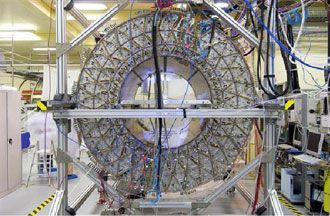
2.2 The ATLAS Detector                                                                             21

Fig. 2.3 The ATLAS detector. The inner-most layers belong to the inner tracker, and include both
silicon and straw tube sensors. Just outside of the inner tracker are the electromagnetic and hadronic
calorimeters. The large air-core toroids and muon spectrometer define the outer envelope of the
detector

counter-clockwise around the ring. The x − y plane is perpendicular to the z axis,
with positive x values pointing towards the center of the ring. The coordinate system
is chosen to be right handed, so the positive y axis points away from the Earth’s
core. ATLAS is nominally symmetric across the x − y plane at z = 0; the portion
of the detector corresponding to z > 0 is sometimes called “Side A”, while z < 0
is called “Side C”. Many subsystems are composed of a barrel portion, which has
detecting elements arranged parallel to the z axis, and two endcap portions, with
detecting elements arranged in planes perpendicular to the beam axis. The endcaps
may therefore be referred to as “Endcap-A” and “Endcap-C” (Fig. 2.3).
    Cylindrical and polar coordinate systems are frequently used to describe both
detecting elements and the trajectories of particles through the apparatus. The radius
R is defined as the perpendicular distance to the z axis. An azimuthal angle φ is
defined around the z axis, while a polar angle θ is defined as the angle away from the
z axis. The variable θ itself is rarely used; rather, a variable known as rapidity (y) is
preferred:
                                        1      E + pz
                                   y = ln                                           (2.3)
                                        2      E − pz

where E represents the energy of an object, and p Z its momentum along the z axis.
In the case of massless objects, such as photons, the rapidity is equivalent to the
pseudorapidity (η):
                                               θ
                                η = − ln tan                                  (2.4)
                                               2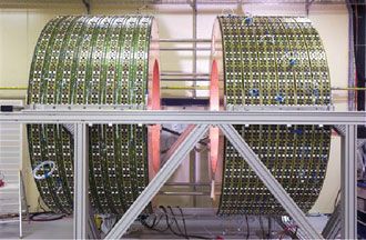
22                                       2 The Large Hadron Collider and the ATLAS Detector

               (a)                                                 (b)

Fig. 2.4 The barrel (a) and endcap (b) inner tracking subsystems of the ATLAS detector. The pixel
subsystem is closest to the beamline, followed by the SCT, and finally the TRT. Detecting elements
in the barrel are arranged axially, while those in the endcap are arranged radially

   As pseudorapidity is defined only with respect to θ, it has a well-defined and mass-
independent interpretation in the lab frame, and is commonly used when discussing
detector performance. It is also common to refer to the η − φ plane, in which the
surfaces of the cylindrical detectors appear as flat sheets.
   Colliding protons transfer momenta through constituent partons which carry
unknown fractions of the proton momentum. Some of that momentum is exchanged
in the hard interaction, and some of it lost to remnants that escape down the
beam pipe. Thus, one cannot easily use total momentum conservation to place
constraints on the kinematics of a single event. However, as the protons approach
each other with trajectories that are nearly along the z axis, momentum is con-
served in the plane transverse to the beam axis. Thus, in many cases, only the trans-
verse component is used when describing object kinematics, e.g. E T (= Esinθ) and
pT (= psinθ).

2.2.2 Inner Tracker

The inner tracker contains three subsystems. The subsystem closest to the interaction
point is composed of silicon pixel sensors, and is commonly called the “pixel detec-
tor” (or just the “pixels”). Just outside of the pixels is a silicon microstrip detector,
called the Semi-Conductor Tracker (SCT). The outermost system is a straw tube
tracker with transition radiation inducing and detecting capabilities, called the Tran-
sition Radiation Tracker (TRT). Each subsystem is composed of a barrel and two
endcaps, shown in Fig. 2.4.
    Silicon-based trackers are used in all modern general-purpose particle detectors
for their excellent position resolution, which is typically on the order of microns.
The sensors are thin pieces of high-purity doped silicon, which produce electron-
hole pairs when traversed by an ionizing particle. An electric field is applied to the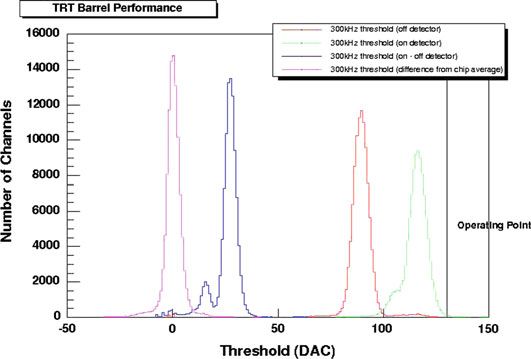
2.2 The ATLAS Detector                                                                  23

sensor to prevent the pairs from recombining, and the subsequent drift and capture of
the free charge carriers produces a current pulse that is read out by analog electronics.
   The pixel and SCT subsystems each provide a small number of hits on track;
the TRT, by contrast, is a straw-tracker that provides semi-continuous tracking out to
large radii. An typical charged particle traversing the TRT will produce approximately
36 hits on track, with a resolution of around 130 µm. The TRT is also unique in its
ability to induce and detect transition radiation, which provides good electron/pion
separation over a broad range of particle momenta.

2.2.2.1 The Pixel Detector

The pixel detector has a barrel section and two endcap sections. The barrel has three
concentric layers, with distances of 50.5, 88.5, and 122.5 mm from the beam axis,
and which cover the central region up to |η| = 1.9. The innermost layer is called
the “B-layer”, and is mechanically integrated with the beryllium beam pipe. There
are three endcap disks on each side, extending the total coverage out to |η| = 2.5.
A charged track originating at the interaction point will almost always produce three
pixel hits; the single-hit efficiency ranges from 97 to 100 %, depending on the layer,
including acceptance losses.
    There are 1,744 “sensors” in the pixel subsystem, with each sensor composed of
47,323 individual pixels. The sensors are 19 × 63 mm2 , while the nominal pixels
dimensions are 50 × 400 µm2 . This leads to a total of over 80 million pixels, each
with an intrinsic R − φ accuracy of 10 µm, and an intrinsic z (R) accuracy of 115 µm
in the barrel (endcap).

2.2.2.2 The Semi-conductor Tracker

The SCT is also composed of a barrel and two endcap sections. The barrel part
has four concentric layers, ranging from an innermost radius of R = 299 mm to
the outermost layer at R = 514 mm. It covers the central region, up to |η| = 1.1. The
endcaps each have nine disks of varying sizes, extending the total coverage of the
SCT out to |η| = 2.5. A charged track originating from the origin will almost always
cross four separate SCT detecting elements; the single-hit efficiency is better than
99 % in all regions of the detector.
    The silicon sensors are designed as collections of thin strips; each of the 15,912
sensors has 768 active strips, for a total of over 6 million channels. The strips are 12 cm
in length, with a pitch of 80 µm. Each layer of the SCT has sensors on both sides, with
a stereo angle of 40 mrad between back-to-back modules. This allows the nominally
one-dimensional sensors to have a resolution in z (R) in the barrel (endcap) of roughly
580 µm, while the resolution in R − φ is 17 µm. The requirement of coincident hits
on both sides of the module reduces the impact of noise to negligible levels.
24 2 The Large Hadron Collider and the ATLAS Detector
2.2.2.3 Transition Radiation Tracker
The Physics of Straw Trackers
When a charged particle passes through the TRT straws, Coulomb interactions
between the charged particle and the valence electrons in the gas will result in the
liberation of some of those electrons from their respective nuclei. In the TRT, the
outer wall of the straw has a radius of 2 mm and acts as a cathode, held at a negative
potential. A wire strung down the middle of the straw acts as an anode. The primary
ionization electrons are move towards the anode; as they get close to the wire, the
strong electric field allows the primary electrons to ionize more of the gas, inducing
an avalanche of electrons that amplifies the signal at the wire. This characteristic
“gas gain” in the TRT is of order 2 × 10⁴ .
If the electrons are liberated close to the wire, the electrons will be collected by the
anode almost immediately. Electrons that are freed closer to the cathode will have a
drift time that depends on the type of gas used—for a Xenon/CO2 mixture, the drift
time for electrons will be around 25 ns/mm. A particle passing through the straw will
always ionize some of the gas close to the edge of the straw, so the “trailing edge”
of the electronic pulse should be fixed with respect to the time at which the particle
traverses the straw.
The electron drift towards the anode is balanced by an ion drift towards the
cathode. The ion drift is largely composed of the ionized gas from the avalanche
near the wire, and thus travels the full 2 mm to the straw wall. This ion drift occurs
at significantly longer time scales (µs/mm) and induces a long tail of mirror current
on the wire. An example of the total straw current response is shown in Fig. 2.5a.
The tail is sufficiently long compared to the LHC bunch spacing that collecting all
of the charge from the ions is not possible at the LHC, so some active cancellation
is performed at the TRT front-end. This is illustrated in Fig. 2.5b, and explained in
more detail in Section “Front-End Electronics”.
Mechanical Design
Like the silicon trackers, the TRT has one barrel and two endcap sections. The barrel
has straw tubes arranged coaxially with the beamline, while the endcaps have straws
arranged radially in layers of constant z. The barrel part provides full coverage out
to |η| = 0.7, and partial coverage up to |η| ≈ 1.0, while the endcap extends the
coverage to |η| = 2.
The straw tubes in the TRT are made of two layers of polyimide film, strengthened
by carbon fibers, surrounded by two thin layers of aluminum protected by a graphite-
polyimide layer. The straws are 4 mm in diameter, and 1.4 m (0.35 m) long in the barrel
(endcap). A gold-plated tungsten wire runs down the middle of the straw, attached to
tension plates on either end. The straws are filled with a gas mixture of 70 % Xe, 27 %2.2 The ATLAS Detector 25
7000
6000 Electron component
5000
Amplitude (μV)
4000
3000
2000
1000 Ion tail
0
25 50 75 100 125 150 175 200 225 250
Time (ns)
(a) (b)
Fig. 2.5 a The current response on the TRT wires due to a point-like ionization in the gas. The
component due to the avalanche electrons is roughly 5 % of the total signal, and quickly gives way
to a long tail due to the ion drift towards the cathode. b The result of the baseline restoration in
the TRT front-end electronics for a 2 fC (solid) and 24 fC (dashed) input charge. The 24 fC pulse is
scaled to have the same peak amplitude as the 2 fC pulse (Images from Ref. [3])
CO2 , and 3 % O2 .2 The Xenon provides efficient absorption of the transition radiation
X-rays, while the CO2 and O2 help to prevent frequent discharges in the gas and
increase the electron drift velocity. The straw wall is held at approximately −1530 V.3
The gold/tungsten wire anode is connected to the analog readout electronics.
There are 298,304 straws in the TRT; 52,544 straws are in the barrel. The wires in
these straws are separated at |η| = 0 with a glass bead, allowing the analog signals
to be read out on both ends, and effectively doubling the total readout channels to
105,088.4 The barrel is split into three concentric layers of 32 trapezoidal modules
each, supported by a carbon-fiber space frame. On either end of each module are
two triangular “active roof” boards, which hold the analog and digital electronics. A
picture of the barrel TRT, taken in its surface assembly facility at CERN, is shown
in Fig. 2.6a.
The remaining 245,760 straws are split evenly between both endcaps. Each endcap
is composed of stacks of disks in z called wheels. The first six wheels in z are the
“A” wheels; each A wheel has sixteen planes of straws. The outermost eight wheels
are the “B” wheels; each B wheel has eight planes of straws.5 Each plane has 768
straws, and the planes in all of the wheels are slightly offset from each other in φ
(with a period of eight planes) to ensure good coverage. The readout electronics are
2 A 70 % Ar/30 % CO2 mixture was used for much of the commissioning period, to avoid the cost
of running with Xenon.
3 The exact voltage is tuned in groups 1̃00 straws to give a gas gain of 2.5 × 10⁴ .
4 The innermost 10 layers in R have two glass beads, creating an uninstrumented gap in the middle
of the straw; this was done to reduce the total occupancy of the innermost straws at high luminosities.
5 The original design of the TRT called for “C” wheels that would extend the |η| coverage out to
almost 2.5; for a number of reasons, these wheels were never built.26 2 The Large Hadron Collider and the ATLAS Detector
(a) (b)
Fig. 2.6 The ATLAS TRT barrel (a) and endcap (b) in their assembly facility on the surface. The
TRT barrel is shown during cosmic-ray testing, when 3/32 of the detector (in φ) were instrumented
and read-out. The endcap is shown before the combination of the A (right) and B (left) wheels into
the full endcap package
connected to the straws at the outer radius of the endcap. Each wheel has 32 slices in
φ; each B-wheel has one front-end board per φ slice, while the A-wheels each have
two boards, stacked in z. A picture of one of the TRT endcaps is shown in Fig. 2.6b.
Transition Radiation
Transition Radiation (TR) is emitted by relativistic particles when they pass between
media with different dielectric constants. The total TR energy emitted, per material
transition, by a relativistic particle with unit charge is:
α
E= γω p (2.5)
3
√
where γ is the Lorentz gamma factor (γ = c/ c2 − v 2 ) and ω p is the plasma
frequency, which depends on the materials at the boundary region. A typical value
of ω p is roughly 20 eV. The transition radiation photons are produced with energies
of several keV—more energy than that produced by minimum ionizing particles
passing through a straw (around 1 keV). As electrons have masses that are 250 times
smaller than pions, the γ factor for an electron with the same energy as a pion will
be significantly larger, corresponding to a larger probability for emitting transition
radiation. The TR photons are also emitted with small angles (θ ≈ 1/γ) relative to
the particle’s direction. Unfortunately, the probability of a TR photon being emitted
is low (from the factor of α/3 ≈ 1/(3 · 137)), meaning many transition regions need
to be encountered to ensure good TR emission efficiency.
In the barrel, the radiator material is a foam mat of polypropylene/polyethylene
fibers [4]. The fibers have a diameter of 19 µm, and are molded into 3 mm-thick
fabric sheets. The sheets are cut in the shape of the barrel modules and stamped with
a hole pattern allowing the straws to be inserted perpendicular to the plane of the2.2 The ATLAS Detector 27 sheet. Around 500 sheets are needed to fill each barrel module. In the endcap, the radiator is made of layers of 15 µm-thick polypropylene foils [5]. The wheels are segmented into groups containing four straw-planes each; stacks of foils were placed at the outside edges of the four-plane wheels, and between each internal straw-plane. The number of foils in each stack ranges from 6 to 34, depending on the position of the stack in z. The emitted transition radiation photons are absorbed by the Xenon gas, producing a cluster of primary electrons. Front-End Electronics The principle components of the front-end electronics are custom made, including the analog and digital application specific integrated circuits (ASICs) and the printed circuit boards on which they are mounted. The analog chips are connected directly to the straw wires, and perform amplifica- tion, shaping, discrimination, and base-line restoration (ASDBLR) of the avalanche current from the wire. The ASDBLR is implemented as a custom ASIC in a radiation- hard process so as to withstand the high radiation background near the interaction point. Signals from the wire pass first through a pre-amplifier, which has a gain of 1.5 mV/fC and a peaking time of 1.5 ns. The signals are then shaped to isolate the electron peak of the ionization curve (see Fig. 2.5a). The ion-tail is canceled and the baseline output restored as the signal is passed into the discriminators. There are two independent discriminators; the first is for detecting the currents from min- imum ionizing particles, and the second is for detecting the larger currents from transition radiation photons. Each discriminator has an associated threshold, set by an externally-applied voltage level, and interpreted with respect to the analog ground reference. The “low” threshold is applied to the first discriminator, in the range of 250–300 eV, while a “high” threshold is applied to the transition-radiation discriminator, usually at 5–7 keV. The output of each channel is a ternary signal, indicating the firing of neither, one, or both of the discriminators (with the ambigu- ity in the second case broken by assuming that the low threshold is always lower than the high threshold). Each ASDBLR has eight channels, each corresponding to a single straw. The discriminator thresholds are shared by all channels in an ASDBLR. The analog output from the ASDBLR feeds directly into a drift time measure- ment read-out chip (DTMROC), which digitizes the analog signals and synchro- nizes them to the 40 MHz clock. The DTMROC, like the ASDBLR, is also a custom ASIC implemented in a radiation-hard process. Each DTMROC takes the output of two ASDBLRs, and provides binary output for the low-level discriminator of each channel in eight time-bins every 25 ns (3.125 ns per bin). The high-level threshold information is encoded as a single bit per 25 ns. The digitized results, along with a counter indicating the bunch crossing associated with the straw data, are stored for up to 6 µs while waiting for a trigger decision. The DTMROCs also store the configuration for each of its ASDBLRs, and apply the low and high thresholds in the form of voltage levels with respect to the digital ground reference.
28                                       2 The Large Hadron Collider and the ATLAS Detector

    In the barrel, both the ASDBLRs and DTMROCs are mounted on the same active
roof (AR) boards. The ASDBLRs occupy the low-z side of the board, while the
DTMROCs are on the opposite side. Each of the three trapezoidal module types in
the barrel have two unique triangular boards per side, for a total of twelve independent
board designs.6 Data to and from the chips pass through a connector on the outer
(DTMROC) side of the AR board.
    In the endcap, the ASDBLRs and DTMROCs are mounted on separate boards. The
ASDBLR boards for the A wheels and B wheels are slightly different in design, to
accommodate the larger gaps between the straw planes in the B-wheels. Each ASD-
BLR board connects to 64 straws through flexible integrated circuits. The DTMROC
boards for the A-wheels and B-wheels are identical, and arranged in triplets. Each
part of the three pieces corresponds to a single ASDBLR board, and all channels on
a triplet share a common connection for signal and power transmission.
    One of the principle challenges in the construction of a straw tracker like the TRT
is the sensitivity of its detecting elements to high frequency noise. To reduce the
impact of noise generated outside of the TRT volume, the digital ground planes of
all AR boards in the barrel are electrically connected to the copper tape wrapping
the carbon fiber space frame, completing a large Faraday shield. In the endcap, the
analog ground plane completes an internal Faraday shield, while an external shield
is created by cable trays between the endcap and the cryostat wall.
    In addition to external noise, the close proximity of the signal traces carrying the
40 MHz clock to the preamplifiers in the ASDBLRs leads to significant clock pickup.
This is especially true in the barrel, where the analog and digital circuits share a single
printed circuit board. Extensive testing was done to ensure that the detector operated
at or below its designed noise occupancy of 2.25 %, while retaining a high tracking
efficiency. This 2.25 % noise occupancy is commonly expressed in terms of a noise
hit rate, which for a 40 MHz clock (and a three bunch-crossing readout window) cor-
responds to 300 kHz. The amount of noise is quantified by the threshold at which this
300 kHz rate is reached. Figure 2.7 shows the 300 kHz rate threshold for all electronics
channels before and after installation on the barrel modules. The left-hand shoulder
in the “on detector” and “on-off detector” trends is due to the “short” straws at low R
(which have an uninstrumented region in the middle of the wire) and indicates that
the detector is operating at the thermal limit defined by the capacitance of the wires.

Back-End Electronics and Data Acquisition

The interface between the TRT front-end electronics and the ATLAS data acquisition
(DAQ) system is composed of a pair of custom 9U VME modules called the Timing
and Trigger Controller (TTC) and Read-Out Driver (ROD). The TTC receives copies

6While the boards that mirror each other across the x − y plane are similar in size and shape, and
have identical numbers of channels, they were designed and implemented separately.
2.2 The ATLAS Detector 29
Fig. 2.7 Per channel 300 kHz threshold distributions for Barrel electronics on (green), off (red),
on–off (blue) the detector and then difference from chip average (purple). Note that the increase in
the 300 kHz threshold when the electronics are mounted in place is due to the detector capacitance
which raises the equivalent noise charge figure for the ASDBLR. The smaller capacitance of the
first nine layers of ‘short’ straws is clearly evident in the difference (blue) distribution (Figure and
caption from Ref. [6].)
of the ATLAS clock and command signals, and distributes them to the front-end
electronics through intermediate “patch panels” (physically located within the muon
spectrometer). The RODs receive data from the front-end, package them, and either
make them available over the VME backplane (for testing) or pass them to the ATLAS
DAQ system over a fiberoptic link.
Upon receipt of a level-1 trigger accept from the TTC, a DTMROC bundles the
hit information from three consecutive bunch crossings and transmits the data to the
TRT backend electronics. The data are transmitted through thin twisted-pair cables
to patch panels, which encode and multiplex the data in groups of 30 DTMROCs.
The data are then transmitted over a 1.2 Gb/s fiberoptic link to the RODs. A graphical
representation of the read-out chain, from front-end to back-end, is shown in Fig. 2.8.
In order to collect front-end data that correspond to the bunch crossing of interest,
the system must be carefully tuned so that the digitized pulses for each straw are
fully contained in a 75 ns window. This is accomplished by tuning the trailing edge
of each digitized pulse to fall near the end of the readout window. As mentioned
previously, a minimum-ionizing particle will always ionize some of the gas near
the straw wall, meaning that the trailing edge of the pulse is primarily determined
by the wire-to-wall distance. The time over threshold for the digital output is then
determined by the point of closest approach of the track to the wire. Figure 2.9 has an
illustration of this effect. An example of the effect of a charged particle track passing
further away from the center of the wire is shown in Fig. 2.10.30 2 The Large Hadron Collider and the ATLAS Detector Fig. 2.8 Half of 1/32nd of the TRT readout chain, from back end modules to the front-end elec- tronics Fig. 2.9 The passage of a charged particle through the straw ionizes gas, which causes electrons to drift into the anode. The resulting current is read out by the analog electronics, and then digitized. The pulse at the right shows the result of that digitization. The blue regions are where the low threshold was crossed—the red region is where both the low and the high threshold were crossed. The point of closest approach of the particle to the wire determines the leading edge of the digital pulse, while the size of the straw (and drift speed of the gas) determines the trailing edge Straw Hit Efficiency for Tracking The hit efficiency for the barrel and endcap detectors are shown in Fig. 2.11 as a function of the distance of closest approach of the charged particle to the straw
2.2 The ATLAS Detector                                                                                                                                   31

Fig. 2.10 A scenario similar to that shown in Fig. 2.9. In this case, the straw is just barely hit by the
charged particle, and the only gas ionized is near the cathode. The trailing edge of the distribution
does not shift, as it is fixed by the size of the straw—the leading edge, however, moves later in time
to reflect the drift radius of the track

                 1                                                                             1
              0.95                                                                          0.95
               0.9                                                                           0.9
                                                                                            0.85
 Efficiency

              0.85                     TRT barrel                                                                    TRT end-caps
                                                                               Efficiency

               0.8                                                                           0.8
                                        Data 2010                                                                     Data 2010
              0.75                                                                          0.75
                                        Monte Carlo                                                                   Monte Carlo
               0.7                                                                           0.7                      Fit to data, ε = 0.946
                                        Fit to data, ε = 0.944
              0.65                                                                          0.65
                                        Fit to Monte Carlo, ε = 0.951                                                 Fit to Monte Carlo, ε = 0.957
               0.6                                                                           0.6
              0.55        ATLAS Preliminary                 s = 7 TeV
                                                                                            0.55        ATLAS Preliminary                 s = 7 TeV
               0.5                                                                          0.5
                     -2    -1.5   -1   -0.5    0      0.5        1   1.5   2                       -2    -1.5   -1   -0.5   0       0.5        1   1.5   2
              Distance from track to straw centre [mm]                                      Distance from track to straw centre [mm]
                                         (a)                                                                           (b)
Fig. 2.11 Plots of the hit efficiencies for the barrel (a) and endcap (b) as a function of the distance
of the track from the straw center. The 2 % of channels known to be dead are not considered

center. The total efficiency, excluding the 2 % of channels known to be dead, is over
95 % in the plateau region.

Transition Radiation Performance

The primary purpose of transition radiation detection is to separate electrons from
charged pions, which complements the separation of electrons from pions based on
the evolution of the shower in the electromagnetic calorimeter (especially at low
particle energies). The different masses of electrons (0.5 MeV) and pions (140 MeV)
mean that electrons and pions with similar momenta will have different Lorentz γ
factors, and thus different probabilities for emitting transition radiation. The tran-
sition radiation turn-on curves measured with the TRT using 2010 data are shown
in Fig. 2.12b, and show the good performance of the detector compared with Monte
Carlo simulations.
32 2 The Large Hadron Collider and the ATLAS Detector
High-threshold probability 0.3 0.3
High-threshold probability
0.25 0.25
ATLAS Preliminary ATLAS Preliminary
0.2 TRT barrel 0.2 TRT end-caps
Data 2010 ( s = 7 TeV) Data 2010 ( s = 7 TeV)
0.15 0.15
Monte Carlo Monte Carlo
0.1 0.1
0.05 0.05
γ factor γ factor
0 0
2 3 4 5 3
10 10 10 10 10 10 10 2 10 10 4 10 5
1 10 1 10 1 10 1 10
Pion momentum [GeV] Electron momentum [GeV] Pion momentum [GeV] Electron momentum [GeV]
(a) (b)
Fig. 2.12 A plot of the transition-radiation turn-on for electrons and pions, as a function of their
Lorentz γ factor, in the barrel (a) and endcap (b). The y-axis is the probability of inducing a high-
threshold hit in the straws. The electron sample is extracted from reconstructed photon conversions,
while the pion sample includes all low-momentum tracks that do not fall in the electron sample
Fig. 2.13 The ATLAS calorimeter subsystems. The EM calorimeter is a lead-LAr accordion sam-
pling detector, while the hadronic calorimeter is composed of steel and scintillating tiles in the
barrel, and copper/LAr in the endcaps
2.2.3 Calorimetry
The barrel part of ATLAS calorimetry system is composed of a high-granularity
lead/liquid-argon (LAr) electromagnetic (EM) sampling calorimeter and a steel/
scintillating-tile hadronic sampling calorimeter. In the endcap, the hadronic calorime-
try is implemented with a LAr design instead of with scintillating tiles. A cut-away
view of the ATLAS calorimeter system is shown in Fig. 2.13.2.2 The ATLAS Detector 33
The EM and hadronic calorimetry provide separate event data for full reconstruc-
tion, but a reduced form of their input is merged in hardware to make Level-1 trigger
decisions with low latency. At Level-1, one speaks of trigger “towers”, composed of
both EM and hadronic components, which measure the energy deposited in an array
of detecting elements pointing outwards from the interaction point.
2.2.3.1 Electromagnetic Calorimeter
The EM calorimeter is of principal importance to the study of photons. Except in the
cases where a photon pair converts in the inner detector (discussed in more detail in
Sect. 4.1.1), the only sign of a photon’s presence is a deposit of energy in the EM
calorimeter.
The ATLAS electromagnetic calorimeter has a lead-LAr accordion design, seen
in cross-section in Fig. 2.14. When a photon enters the detector, it interacts with the
lead plates and pair-produces an electron and a positron. The electron and positron
continue to interact with the material in the calorimeter, producing bremsstrahlung
photons, which in turn pair-produce, creating a “shower” of electromagnetic activity.
The LAr medium samples the energy of the shower, which is read out by analog
electronics through capacitively-coupled copper sheets at the edges of the absorber.
An electron entering the LAr calorimeter will undergo the same chain reaction as
a photon. Distinguishing between electrons and photons solely by the shower profile
is difficult, and is not attempted at reconstruction level. Instead, the presence of a
matching track in the inner detector is used to break the ambiguity. The situation is
somewhat complicated in cases where a photon pair-produces before reaching the
calorimeter; this will be discussed further in Sect. 4.1.1.
The LAr calorimeter is separated longitudinally into four layers. The baseline
granularity of the calorimeter cells in the barrel is 0.025 × 0.025 in η × φ; all
cells have sizes that are even multiples (or fractions) of this baseline.7
• The first layer (at lowest R), called the pre-sampler, is a thin layer of active LAr
that is designed to estimate and correct for losses of energy through a particle’s
interaction with material upstream of the calorimeter (i.e. in the inner tracker).
It only extends to |η| = 1.8, and does not absorb a significant amount of a
particle’s energy. The detecting elements are 0.025×0.1 in size, with a coarser
granularity in φ.
• The next layer out in radius is often called the “strip” layer, as it is composed of
thin strips in η that provide excellent position resolution, as well as the ability to
discriminate between single and double pulses (corresponding to single photon
and diphoton objects, respectively). Each strip has a size of 0.025/8 × 0.1, in
the barrel, and similar sizes in the endcap (that vary slightly with |η|).
7The length in φ is sometimes quoted as 0.025 and sometimes as 0.0245; in reality, it is defined as
2π/256 = 0.02454 . . . .34 2 The Large Hadron Collider and the ATLAS Detector
Towers in Sampling 3
= 0.0245 0.05
Trigge
r Towe
Δη = 0 r
2X0 .1
η=0
m
0m
47 16X0
Trigge
Tow r
Δϕ = 0er
.0982
4.3X0
m
m
1.7X0
00
Δϕ=0.0
15
245x
36.8m 4
mx
=147.3 4
mm Square towers in
Sampling 2
Δϕ = 0
.0245
ϕ
37.5m Δη = 0
m/8 = .025
4
Δη = 0 .69 mm
.0031
Strip towers in Sampling 1
η
Fig. 2.14 The granularity of the liquid argon electromagnetic barrel calorimeter, shown near η = 0.
The innermost layer shown here is the ’strip’ layer, with fine segmentation in η. The primary
sampling layer makes up the bulk of the calorimeter volume and material, while the third (outer)
layer has the coarsest granularity
• The following layer is the primary sampling layer, typically called “layer 2”
(where the presampler is “layer 0”). Each cell in the second layer is 0.025 ×
0.025 in η ×φ. The bulk of the energy of the shower is deposited in layer 2.
• The final layer, called “layer 3”, is used to estimate the amount of energy
that was not contained in the second layer, and has a coarser granularity of
0.050 × 0.025.
The fine segmentation of the EM calorimeter provides good position resolution
for electron and photon reconstruction. After calibration, the η resolution in the strips
is roughly 3 × 10⁻⁴ , while the resolution in φ is between 5 × 10⁻⁴ and 2 × 10⁻³
radians, depending on η.8 √
The design energy resolution of the EM calorimeter is σ E /E = 10 %/ E ⊕ 0.7%,
where the last term (0.7 %) corresponds to the “constant term”, and is independent of
energy. A combination of studies using simulated data and test beam results indicate
8 The precision in φ is degraded by the presence of material in the ID, which induces bremsstrahlung
for electrons and pair production for photons.2.2 The ATLAS Detector 35
3 3 3 3 3 3
2.8 2.8 2.8
2 2.6 2 2.6 2 2.6
1 2.4 1 2.4 1 2.4
Status
Status
2.2 2.2 2.2
Status
0 0 2 0 2
φ
φ
2
φ
1.8 1.8 1.8
-1 -1 1.6 -1 1.6
1.6
-2 1.4 -2 1.4 -2 1.4
1.2 1.2 1.2
-3 1 -3 1 -3 1
-1.5 -1 -0.5 0 0.5 1 1.5 -3 -2 -1 0 1 2 3 -3 -2 -1 0 1 2 3
η η η
(a) (b) (c)
Fig. 2.15 Maps of the dead front-end board optical links for the presampler (a), first sampling (b),
and second sampling (c) of the LAr calorimeter. Photon candidates that fall into the red regions are
ignored
that the calorimeter is meeting its performance goals [7], and results with early col-
lision data confirm this [8].
The transition region between the barrel and endcap portions of the EM calorime-
ter contains an uninstrumented gap, needed to connect the inner tracker with services
outside of the cryostat. Electron or photon candidates that fall within this gap will
have reduced energy and position resolutions, and are excluded from most analy-
ses. Furthermore, the strips in the first layer only extend to |η| = 2.37. Therefore,
photon candidates are required to satisfy the fiducial requirement |η S2 | < 1.37 or
1.52 ≤ |η S2 | < 2.37, where η S2 is the η of the cluster barycenter in the second
sampling layer.
Finally, a problem with the optical links that transmit data to and from the LAr
front-end electronics prevented certain parts of the EM calorimeter from being prop-
erly read-out during the 2010 run.9 The (η, φ) maps of the dead readout optical links
for the presampler, first and second sampling layers are shown in Fig. 2.15. Events
in which the leading photon is found within one of the red regions in those plots are
excluded from the analysis; the effect of this acceptance loss is discussed in Chap. 5.
2.2.3.2 Hadronic Calorimeter
The hadronic calorimeter is composed of three independent pieces: the Tile Calorime-
ter (TileCal), which covers the central region up to |η| = 1.7; the liquid-argon
hadronic endcap (HEC), which covers 1.5 < |η| < 3.2; and the liquid-argon for-
ward calorimeter (FCal), which extends the total acceptance beyond the HEC to
|η| < 4.9. The acceptance for photons is driven by the EM calorimeter, so only the
TileCal and the HEC are described in detail here. They are√ both sampling calorime-
ters, with nominal energy resolutions of σ E /E = 50 %/ E ⊕ 3 % for |η| < 3.2.
The primary function of the hadronic calorimeter for photon studies is to provide
a measurement of the hadronic activity behind the cluster in the EM calorimeter. Real
photons will deposit very little energy in the hadronic calorimeter, having left most
9 This problem has since been fixed, restoring the full acceptance in 2011.36 2 The Large Hadron Collider and the ATLAS Detector
(if not all) of their energy in the liquid-argon calorimeter. Tight cuts on the allowed
amount of hadronic energy associated with the photon cluster help to reduce the
background contamination of the signal sample—these cuts are described in detail
in Sect. 4.2.
TileCal
The TileCal has a barrel region (|η| < 1.0) and two “extended barrel” regions (0.8 <
|η| < 1.7). It has steel absorbers and active elements made from scintillating tiles.
The radial thickness of the detector is roughly 7.4 nuclear interaction lengths.10
The tiles themselves have a granularity of 0.1×0.1 in η×φ. They are arranged
in towers with a projective geometry in η, pointing towards the interaction point. The
scintillators are read-out with photomultiplier tubes, which provide analog signals
that are digitized on the front-end and made available for both triggering and readout.
Hadronic End Cap
The HEC is an extension of the liquid-argon calorimeter, with copper-plate absorbers
and a liquid-argon active medium. Each endcap is composed of two wheels, each
divided into two segments in depth. Like the TileCal, the granularity of the detecting
elements is 0.1 × 0.1 in η × φ out to |η| < 2.5; for 2.5 < |η| < 3.2, the detecting
elements measure 0.2 × 0.2.
2.2.4 Trigger
ATLAS has a three-tiered trigger system, designed to select interesting events with
a final output rate of roughly 200 Hz. It consists of a hardware trigger in the first tier
(Level-1), followed by a software trigger that performs partial event reconstruction
(Level-2). The final tier (the Event Filter) performs full event reconstruction using the
same tools as used for offline analysis, albeit with a modified set of algorithms. The
second and third tiers are collectively known as the High Level Trigger. A schematic
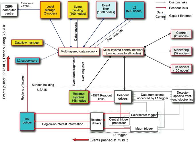
view of the ATLAS trigger system is shown in Fig. 2.16.
Both Level-1 and Level-2 are Region of Interest (RoI) based triggers: they only
consider the data from detecting elements in a limited region of η and φ. This allows
them to make decisions before the data from all of the different subsystems and RoIs
are built into a full event record, reducing the total internal bandwidth used by the
10The nuclear interaction length, λ, of some material defines the mean distance over which the
number of relativistic charged particles is reduced by a factor of 1/e as they pass through that
material.2.2 The ATLAS Detector 37 Fig. 2.16 A schematic view of the ATLAS trigger and data-acquisition systems. Data flows from the bottom-right to the top-left system. The event filter operates after full events are built, and is the only place where the trigger can consider complicated event topologies spanning multiple RoI’s.11 2.2.4.1 Level-1 Hardware Trigger The Level-1 trigger is a logical OR of many input trigger signals, combining infor- mation from the calorimeter and muon systems. Decisions are made by the individual trigger subsystems within 2.5 µs of the relevant bunch crossing, and are then prop- agated to the central trigger processor (CTP), which makes the final Level-1 trigger decision and distributes it to all ATLAS subsystems. After each Level-1 accept, there is a minimum dead-time of five bunch crossings (125 ns). The total propagation delay, from a proton–proton collision to the readout of the detecting elements on the front- end, is less than 4 µs. The event data are then transmitted from the front-end to RODs, which package the event data for a large number of channels and transmit the formatted data into rack-mounted computers equipped with fiberoptic input cards (ROSs). The ROSs buffer the event data until it is requested by the Level-2 trigger or by the Event Building system. 11 Exceptions to this rule include triggers based on E Tmiss , which do exist at Level-1 and Level-2.
38                                     2 The Large Hadron Collider and the ATLAS Detector

   The Level-1 accept rate is designed to be 75 kHz, almost three orders of magnitude
below the 40 MHz bunch crossing rate. Operating under special conditions, all sub-
systems in ATLAS can accommodate up to a 100 kHz Level-1 accept rate (though
this sometimes requires the truncation of some detector data in order to meet the
bandwidth requirements).

2.2.4.2 Level-2 Software Trigger

The Level-2 trigger is seeded by the Level-1 trigger, and uses a modified set of offline
reconstruction algorithms to refine the Level-1 selection criteria. Level-2 makes use
of the same RoI flagged by Level-1, but takes advantage of the reduced event rate to
run tracking algorithms for the first time, and to evaluate calorimeter quantities with
greater precision. The Level-2 accept rate is limited to 3.5 kHz, with a latency of
roughly 40 ms. Events rejected at Level-2 are flushed from the ROS’s, while events
accepted by Level-2 are then collected by the event-building system, which merges
the event data and passes it to the Event Filter.

2.2.4.3 Event Filter

At the Event Filter, events undergo full reconstruction. The Event Filter uses fast
versions of offline reconstruction tools to look for diphoton and dilepton events,
other multi-object events, and events with significant E Tmiss , in addition to the single-
object topologies that are the focus of the first- and second-level triggers. The final
output rate of the event filter is designed to be 200 Hz,12 with a total latency of
roughly 4 s.

2.2.5 Luminosity

2.2.5.1 Luminosity Measurements

The integrated luminosity is a crucial component of a cross section measurement.
ATLAS has several ways of measuring the luminosity of the LHC beams [9]; for
the 2010 dataset, an event counting technique was used, with the absolute calibra-
tion provided by a series of van der Meer scans taken in April and May of 2010.
The uncertainty on the measured luminosity for early data was 11 %; this has since
improved to 3.6 % for the 2010 dataset [10].

12 The limitation comes from the amount of data the collaboration is willing to keep for later
analysis. In 2010, the nominal maximum output rate was often exceeded.
2.2 The ATLAS Detector                                                                         39

2.2.5.2 Luminosity Blocks

As an LHC fill progresses, the instantaneous luminosity slowly degrades, creating
different conditions at the beginning and end of a fill. The concept of “luminosity
blocks” allows ATLAS to subdivide a run into many separate chunks, within which
all events have similar luminosity conditions.

References

 1. A. Breskin, R. Voss, The CERN Large Hadron Collider: Accelerator and Experiments (CERN,
    Geneva, 2009)
 2. G. Aad et al., The ATLAS experiment at the CERN large hadron collider. J. Instrum. 3, S08003
    (2008) (Also published by CERN Geneva in 2010, p. 437)
 3. ATLAS Collaboration, ATLAS inner detector: technical design report. Vol. 2, CERN-LHCC-
    97-17 (1997)
 4. E. Abat et al., The ATLAS TRT barrel detector. J. Instrum. 3, P02014 (2008)
 5. E. Abat et al., The ATLAS TRT end-cap detectors. J. Instrum. 3, P10003 (2008)
 6. E. Abat et al., The ATLAS TRT electronics. J. Instrum. 3, P06007 (2008)
 7. ATLAS Collaboration, Electron and photon reconstruction and identification in ATLAS:
    expected performance at high energy and results at 900 GeV, ATLAS-CONF-2010-005 (2010).
    http://cdsweb.cern.ch/record/1273197
 8. T.A. Collaboration, Calibrated Z → ee invariant mass, ATL-COM-PHYS-2010-734       √ (2010)
 9. ATLAS Collaboration, G. Aad et al., Luminosity determination in pp collisions at s = 7 TeV
    using the ATLAS detector at the LHC. arxiv:1101.2185 [hep-ex] (Submitted to Eur. Phys. J. C)
10. T.A. Collaboration, Updated luminosity determination in pp collisions at root(s) = 7 TeV using
    the ATLAS detector. Technical report, ATLAS-CONF-2011-011, CERN, Geneva, March 2011
You can also read